A compiler and simulator for partial recursive functions over neural

A compiler and simulator for partial recursive functions over neural networks João Neto1, José Félix Costa2, Paulo Carreira3, Miguel Rosa4 1 Departamento de Informática, Faculdade de Ciências da Universidade de Lisboa, C5 – Piso 1, 1700 Lisboa, PORTUGAL [email protected] 2

Departamento de Matemática, Instituto Superior Técnico, Av. Rovisco Pais, 1049-001 Lisboa, PORTUGAL [email protected] 3

OBLOG Software S.A., Alameda António Sérgio 7-1A 2795-023 Linda-a-Velha PORTUGAL [email protected] 4

Fundação para a Computação Científica Nacional Av. do Brasil, 101. 1700-066 Lisboa. PORTUGAL [email protected]

Abstract. In [6] and [8] it was shown that Artificial Recurrent Neural Networks have the same computing power as Turing machines. A Turing machine can be programmed in a proper highlevel language - the language of partial recursive functions. In this paper we present the implementation of a compiler that directly translates high-level Turing machine programs to Artificial Recursive Neural Networks. The application contains a simulator that can be used to test the resulting networks. We also argue that these experiments provide clues to develop procedures for automatic synthesis of Neural Networks from high-level descriptions.

1. Introduction The field of Artificial Recurrent Neural Networks (ARNNs) is meeting a lot of excitement nowadays. Both because of their achievements in solving real world problems and their simplicity of the underlying principles that still allow them to mimic their biological counterparts. All this excitement attracts people from many different fields such as Neurophisiology and Computer Science. We introduce our subject from a Computer Science perspective. The view we are interested in, is the one in which an ARNN can be seen as a computing mechanism able to perform some kind of computation based on a program coded as a specific arrangement of neural artifacts, like neurons and synapses. This work implements a compiler and a simulator based on the previous Turing Universality of Neural Nets (Revisited) paper, [4]. In [3], [7] and [5] similar ideas are given but they are based on higher level languages. We start by giving the underlying theoretical context on which it is based. In section 2 we give a brief review of the concept of partial recursive function. In section 3 we present our approach for constructing

neural networks from partial we adapted the design of [4] 5 refers to the simulator and paper. The simulator is netdef/nwb.html.

recursive functions. The explanation of how into a compiler is given in section 4. Section usage examples and section 6 concludes this freely available at www.di.fc.ul.pt/~jpn/

2. Partial Recursive Function theory When informally speaking of a neural computer, one could be motivated about what could it be like the language to program such a machine. The language that we will use is the one of partial recursive functions (PRF). Although primitive when compared to modern computer languages, it is simple and powerful enough to program any mechanism with same computing power as a Turing machine. Surely, building complex programs with this language would be very difficult and more appropriate languages exist. For our purposes however, this language is suited. The PRF theory identifies the set of computable functions with the set of partial recursive functions. We shall use a(x1,…,xn) ≡ b(x1, …, xn) to denote equality of the expressions a(x1,…,xn) and b(x1,…,xn), if and only if both a(x1, …, xn) and b(x1, …, xn) are defined for all (x1, …, xn) or both undefined. The axioms also called primitive functions are: • W that denotes the zero-ary constant 0; • S that denotes the unary successor function S(x)=x+1; • U(i,n) that for i and n fixed, 1≤i≤n, denotes the projection function Ui,n(x1, ..., xn) = xi. The construction rules are: • C, denoting composition. If f1, …, fk are n-ary PRFs, and g is a k-ary PRF, then the function h defined by composition, h(x1, …, xn) ≡ g(f1(x1, …, xn), …, fk(x1, …, xn)), is a PRF; • R, denoting recursion. If f is a n-ary PRF and g is a (n+2)-ary PRF, then the unique (n+1)-ary function h, defined by 1) h(x1,…, xn, 0) ≡ f(x1,…,xn) and 2) h(x1,…, xn, y+1) ≡ g(x1,…,xn, y, h(x1,…, xn, y)); is a PRF; • M, denoting minimalisation. If f is a (n+1)-ary PRF, then h(x1,…, xn) ≡ µy(f(x1,…, xn, y)=0) is also a PRF, where

least y such that f(x1,..,xn,y)=0 and ∀z≤y: f(x1,…,xn,z) is defined µy(f(x1,…, xn, y)=0) =  undefined, otherwise For instance, f(x,y)=x+1 is a PRF and is described by the expression C(U(1,2),S). The function f(x,y)=x+y is also a PRF described by the expression R(U(1,1),C(U(3,3),S). In fact, it can be shown that every Turing computable function is a PRF. More details on PRF theory can be found in [1] or [2].

3. Coding PRF into ARNNs Finding a systematic way of generating ARNNs from given descriptions of PRF’s greatly simplifies the task of producing neural nets to perform certain specific tasks. Furthermore, it also gives a proof that neural nets can effectively compute all Turing computable functions as treated in [4]. In this section we briefly describe the computing rule of each processing element, i.e., each neuron. Further we present the coding strategy of natural numbers to load the network. Finally, we will see how to code a PRF into an ARNN. 3.1 How do the processing elements work? Like in [4] we make use of σ-processors. In each instant t each neuron j updates its activity xj in the following non-linear way: xj(t+1) = σ(

N

M

i=1

k=1

∑ ajixi(t) + ∑ bjkuk(t) + cj )

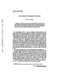
where aji, bjk and cj are rational weights; N is the number of neurons, M the number of input streams uk; and σ is the continuous function defined below:  1 , x≥1 σ(x) =  x , 00

h(...) –1

–1

10

–0.9

0.1

0.1

Y

fig. 4 – Minimalisation. –1 2

IN

=1 if x=0

2 –0.1

–100

–2

x 100

=1 if x>0

fig. 5 – The signal (Sg) network. For each PRF expression an ARNN is generated using the structure of the expression. The construction of the ARNNs is made in a top-down fashion, beginning with the outermost ARNN and then continuously instantiating ARNNs until reaching the axioms. For an expression R(U(1,1),C(S,U(3,3)) we would first build the network for the recursion, then instantiate with the projection axiom network and with the composition rule network, that in turn would accommodate the successor and projection axiom networks. This instantiation mechanism for the network schemas consists of replacing the boxes by compatible network schemas. A box is said to be compatible with a network schema if the number of inputs (respectively outputs) of the box is the same as the number of inputs (respectively outputs) of the network schema. The substitution operation of a box by a network schema consists of connecting the box inputs (respectively outputs) to the network inputs (respectively outputs).

4. Putting the pieces together and building the compiler The tool we want to present to the user, should be capable of handling more complex functions than the simple examples used in the previous sections. Specifying a more complex function implies writing a more complex expression. This motivates the use of a modular and yet simple language to increase readability.

A PRF description is a sequence of statements where each statement is a pair that contains an identifier and an expression. The identifiers label the statement of an associated expression. Each expression is written in the language of PRF described in section 2 (recursive application of rules to rules and axioms) and may reference a previous statement. For example, when specifying the product PRF we can initially write the statement for the sum PRF and follow it by a shortened product PRF expression in which the sum expression is substituted by the initial sum identifier as shown below. sum R(U(1,1), C(U(3,3), S)) product R(Z, C(U(3,3), U(1,3), sum)) The idea is to write further expressions making use of the previously defined ones. A more detailed example is given in section 5.

5. Using the simulator and compiling examples An application was built to provide the user not only with a compiler of PRF into ARNNs but also a simulator that among other things allows stepby-step simulation and inspection groups of neurons. In our application there are two modes of building ARNNs: by compiling the PRFs or by reading the dynamic equations system that define the neural network. We do not only allow the storage of PRF description, but also of compiled PRF in order to avoid recompiling and to provide input to other simulation tools. The simulator takes the already built ARNN and configures it to read the input. Then it requests each neuron to process data. This process is iterated until a signal is seen in the OUT line of the outmost network. During the ARNN computation, the program allows the user to inspect the computations that are taking place inside the net, being able to select some sets of neurons and customise the animation. The user can also see the corresponding equation of each neuron and define a limit for the number of iterations. To each neuron is given a name by the compiler with special meaning. The name of each neuron expresses particular information on the neuron we are working with, in the following way: • Func is one of W, S, U(i,j), R, C, M. • Type is one or more of the following: In – Stands for the IN line supporting neurons. Out – Stands for the OUT line supporting neurons. Data – Stands for neurons that receive parameters from external networks or that send result of computation to other networks. Res – Stands for neurons that handle results of functions. Hid – Stands for neurons not in one of the border layers. • Num is the number of the neuron inside its network schema. • Depth is the same as the depth in the corresponding PRF parsing tree. • Id is used to ensure an unique identifier for each neuron.

Some examples of function descriptions are given in the table below: Function f=0 f(x)=x+1 f(x,y,z)=y f(x)=0 f(x,y,z)=z+1 f(x,y)=x+y f(x,y)=x*y f(x)=x! f(x)=xy f(x)=sg(x) f(x,y)=x-1 f(x,y)=x-y f(x,y)=|x-y| f(x,y)=min(x,y) f(x,y)=max(x,y) f(x,y)=rm(x,y) f(x,y)=x|y f -1 (y)

Expression W S U(2,3) R(W, U(2,2)) → also called Z C(U(3,3),S) R(U(1,1),z+1) R(Z,C(U(3,3),U(1,3),x+y)) R(C(Z,S),C(U(2,2),C(U(1,2),S),x*y) R(C(Z,S),C(U(1,3),U(3,3),x*y) R(C(W,S),C(W,U(1,2))) R(W,U(1,2)) R(U(1,1),C(U(3,3),x-1)) C(x-y,C(U(2,2),U(1,2),x-y),x+y) C(U(1,2),x-y,x-y) C(C(x-y,x+y),C(C(x-y,x+y),C(x-y,xy),x-y),x+y) R(Z,C(C(U(3,3),S),C(C(U(1,3),C(U(3,3) ,S),|x-y|),sg),x*y)) C(rm,sg) M(C(C(C(U(2,2),fx),U(1,2),|x-y|),sg)

As an example, let us consider the following description of the sum function: proj/1 U(1,1) proj/2 U(3,3) comp C(proj/2,S) sum R(proj/1,comp)

After the compilation of these four statements we have an ARNN with 39 neurons and 70 synapses. Below are presented the first lines of the dynamic equation system: XRin_1_0(i+1) = σ(Ein(i)) XRhid2_1_1(i+1) = σ(XRin_1_0(i)) XRhid3_1_2(i+1) = σ(0.1*XRin_1_0(i) + XRhid3_1_2(i) + XRhid4_1_3(i) - XRhid5_1_4(i) - XREout_1_15(i)) XRhid4_1_3(i+1) = σ(0.1*XRhid3_1_2(i) + XRhid5_1_4(i) - 0.9) XRhid5_1_4(i+1) = σ(XRhid6_1_5(i)) XRhid6_1_5(i+1) = σ(XSout_4_7(i)) XRhid7_1_6(i+1) = σ(XRhid3_1_2(i) + XRhid15_1_14(i) 1) XREres_1_7(i+1) = σ(XRhid13_1_12(i) + XRhid19_1_18(i) - 1) ...

The simulator is freely available at www.di.fc.ul.pt/~jpn/netdef/nwb.html.

6. Conclusion We hope to have taken one step further in understanding the relationship between programming languages and ARNNs. We started presenting a theoretical framework of a very simple programming language. Next, we described a systematic way of obtaining ARNNs from programs written in the presented language and concluded with the presentation of a tool where one can get a practical insight of the presented results. Although the ideas here contained may seem oversimplified when facing real-world applications, adapting them to other more elaborate frameworks like those of process calculi appears to be straightforward. Finally, we also defend that the search for a language more suited to the architecture of ARNNs can give us fresh views on efficient approaches for systematic construction of ARNNs.

References 1. Boolos, G. and Jeffrey, R., Computability and Logic (second edition), Cambridge University Press, 1980. 2. Cutland, N., Computability – An introduction to recursive function theory, Cambridge University Press, 1980. 3. Gruau, F., Ratajszcza J., and Wiber, G., Fundamental study – A Neural Compiler, Theoretical Computer Science, Elsevier, 141, 1995, 1-52. 4. Neto, J., Siegelmann, H., Costa, J., and Araújo, C., Turing Universality of Neural Nets (Revisited), Proceedings of Computer Aided Systems Theory – EUROCAST’97, 1997. 5. Neto, J., Siegelmann, H., and Costa, J., Symbolic Processing in Neural Networks, to be published at the Journal of Brasilian Computer Society, 2001. 6. Siegelmann, H. and Sontag, E., On The Computational Power of Neural Nets, Journal of Computer and System Sciences, Academic Press, [50] 1, 1995, 132-150. 7. Siegelmann, H., On NIL: The Software Constructor of Neural Networks, Parallel Processing Letters, [6] 4, World Scientific Publishing Company, 1996, 575-582. 8. Siegelmann, H., Neural Networks and Analog Computation, Beyond the Turing Limit, Birkhäuser, 1999.