a component architecture for artificial neural network ... - CiteSeerX

A COMPONENT ARCHITECTURE FOR ARTIFICIAL NEURAL NETWORK SYSTEMS

Fábio Ghignatti Beckenkamp

Dissertation zur Erlangung des akademischen Grades Doktor der Naturwissenschaften (Dr.rer.nat.) an der Universität Konstanz eingereicht in der Mathematisch-Naturwissenschaftlichen Sektion im Fachbereich Informatik und Informationswissenschaft

Juni 2002

University of Constance Computer & Information Science

Software Research Laboratory A Component Architecture for Artificial Neural Networks Fábio Ghignatti Beckenkamp June 2002 Page 2

Acknowledgements I dedicate this work to my parents Valecy and Jalda that have made the education of their kids their first priority in life. I express my most profound gratitude to my wife Ana who supported my initiatives and goals from the beginning of our relationship, though it meant even sometimes being geographically separated but close enough for love. Special thanks go to my advisor Prof. Dr. Wolfgang Pree for providing the opportunity of doing this work, and for his expertise, enthusiasm and friendship that helped in the course of doing the PhD. Thanks to my brother Tarcísio and my sister Mariele for being nearby whenever I needed. Thanks to Ana’s family for having comprehended the importance of this effort. This work would not have being possible without the direct support of many people and institutions for several reasons. My thankfulness goes to the University of Constance, its professors, colleagues and staff; and to the Federal University of Rio Grande do Sul, especially to Prof. Dr. Paulo Engel. Some people filled my life during this time with unconditional friendship and help, this includes: Sergio Viademonte; Altino Pavan; Egbert Althammer; André Ghignatti and the Mercador colleagues; Michael Beckenkamp and family; César De Rose; Gustavo Hexsel; Ênio Frantz; Beatriz Leão; Miguel Feldens; Brazilian friends in Germany and European friends.



Deutsche Zusammenfassung Diese Arbeit stellt zuerst die Architekturbausteine eines Komponentenframeworks dar, das im Rahmen der Dissertation implementiert wurde und das die Wiederverwendung der Kernteile von Modellen für künstlichen neuronalen Netze (artificial neural networks, ANN) erlaubt. Obwohl es eine Reihe von verschiedenen ANN-Modellen gibt, wurde ein wesentlicher Aspekt bisher kaum untersucht, nämlich der der Bereitstellung von wiederverwendbaren Komponenten, die eine effiziente Implementierung von entsprechende Systemarchitekturen für diese Domäne ermöglichen. Das Komponentenframework wird mit bestehenden Implementierungsansätzen für ANN-Modelle und -Simulationen verglichen. Die Anwendung von ANN sieht sich mit Schwierigkeiten konfrontiert, wie zum Beispiel Begrenzungen von Hardwareressourcen und passende Softwarelösungen. Die Tatsache, wie sich die ANN-Komponenten die Parallelisierung von vernetzten Computern zunutze machen, stellt einen Beitrag zum Stand der Technik im mobilen Code und in verteilten Systemen dar. Die Software-Architektur wurde so definiert, dass sie die Parallelisierung sowohl der internen Ausführung eines ANNs wie auch der Simulation von unterschiedlichen ANNs, simultan auf derselben Maschine oder auf unterschiedlichen Maschinen verteilt, erleichtert. Das kombinatorische Netzmodell (combinatorial network model, CNM) wurde dabei als Fallstudie für die Implementierung von Parallelität auf der Ebene der ANN-Struktur gewählt. Die durchgeführte Verbesserung eines der ANN-Modelle, nämlich des CNM, stellt einen Beitrag zum Bereich der ANNs selbst und zum Data-Mining dar. Der ursprüngliche CNM-Algorithmus konnte erheblich verbessert werden hinsichtlich der Optimierung des Suchraumes, mit dem Effekt einer höheren Ausführungsgeschwindigkeit und weniger Speicherverbrauch. Das letzte Kapitel bietet einen Überblick über offene Forschungsfragen, die während der Dissertation aufgetaucht sind.

Schlüsselwörter: Framework, Komponenten, Wiederverwendung von Software, objektorientiertes Design, objektorientierte Architektur, künstliche neuronale Netze, intelligente Expertensysteme, hybride intelligente Systeme.



Abstract The main focus of the PhD thesis is about automating the implementation of artificial neural networks (ANNS) models by applying object/ and component technology. Though various ANN models exist, the aspect of how to provide reusable components in that domain for efficiently implementing adequate system architectures has been barely investigated. The prototypical component framework that was designed and implemented in the realm of the dissertation is compared to existing approaches for generically implementing ANN models and simulations. The application of ANNs faces difficulties such as limits of hardware resources and appropriate software solutions. How the ANN components harness parallelization on networked computers represents a contribution to the state-of-the-art in mobile code and distributed systems. The software architecture was defined in a way to facilitate the automated parallelization at the level of the inner execution of an ANN and at the level of the simulation of different ANNs at the same time, on one computing node or on different computing nodes in a distributed way. The Combinatorial Network Model (CNM) was chosen as case study for implementing parallelism at the level of the ANN structure. The improvement of one of the ANN models, namely the CNM, represents a contribution to the area of ANNs itself and to data mining. The original CNM algorithm could be significantly enhanced regarding the aspect how it deals with the search space, which results in a faster execution and less memory allocation. A sketch of research issues that result from the PhD work rounds out the thesis. Keywords: artificial neural networks, object-oriented frameworks, components, software reusability, object-oriented design, software architectures, intelligent decision support systems, hybrid intelligent systems.



Summary A COMPONENT ARCHITECTURE FOR ARTIFICIAL NEURAL NETWORK SYSTEMS ........ 1 ACKNOWLEDGEMENTS ...................................................................................................................... 2 DEUTSCHE ZUSAMMENFASSUNG .................................................................................................... 2 ENGLISH ABSTRACT ............................................................................................................................ 4 SUMMARY................................................................................................................................................ 5 LIST OF FIGURES................................................................................................................................. 10 LIST OF TABLES................................................................................................................................... 13 LIST OF SOURCE CODE EXAMPLES .............................................................................................. 15 ACRONYMS ........................................................................................................................................... 16 1

2

INTRODUCTION ........................................................................................................................... 18 1.1

MOTIVATION ............................................................................................................................ 18

1.2

PROBLEM STATEMENT ............................................................................................................ 18

1.3

OVERVIEW OF THE PROPOSED SOLUTION ............................................................................ 19

1.4

ORGANIZATION OF THE THESIS ............................................................................................. 20

1.5

STATEMENT OF GOALS AND CONTRIBUTIONS ..................................................................... 21

CONTEXT AND STATE-OF-THE-ART...................................................................................... 24 2.1

BIOLOGICAL MOTIVATION ..................................................................................................... 24

2.1.1 2.1.1.1 2.1.2

2.2

The generic artificial neuron ............................................................................................. 25 Activation function ........................................................................................................ 27 ANN Architectures ............................................................................................................. 30

2.1.2.1

Single-Layer Feedforward Networks ............................................................................. 30

2.1.2.2

Multi-Layer Feedforward Networks .............................................................................. 30

2.1.2.3

Recurrent Networks ....................................................................................................... 31

2.1.2.4

Lattice Networks............................................................................................................ 32

ANN LEARNING ALGORITHMS ............................................................................................... 33

2.2.1

Hebbian Learning.............................................................................................................. 34

2.2.2

Competitive Learning ........................................................................................................ 35

2.2.3

Error Correction Learning ................................................................................................ 35


2.2.4

Reinforcement Learning .................................................................................................... 36

2.2.5

Stochastic Learning ........................................................................................................... 37

2.3

ANN INPUT AND OUTPUT DATA ............................................................................................ 37

2.4

CHOSEN ANN MODELS ........................................................................................................... 39

2.4.1

The Backpropagation ........................................................................................................ 40

2.4.2

The Combinatorial Neural Model...................................................................................... 46

2.4.2.1

The IRP learning............................................................................................................ 50

2.4.2.2

The SRP learning ........................................................................................................... 51

2.4.3

The Self-Organizing Feature Maps ................................................................................... 52

2.4.4

The Adaptive Resonance Theory ....................................................................................... 56

2.4.4.1 2.5

The ART1 ...................................................................................................................... 58

SOFTWARE ENGINEERING ISSUES.......................................................................................... 67

2.5.1

Software Quality ................................................................................................................ 67

2.5.2

Flexible software ............................................................................................................... 68

2.5.2.1

Flexibility based on data ................................................................................................ 68

2.5.2.2

State of the art programming concepts........................................................................... 69

2.5.3

3


Framework construction patterns...................................................................................... 73

2.5.3.1

Hook combination patterns ............................................................................................ 74

2.5.3.2

Construction principles and the GoF design-patterns .................................................... 76

2.5.4

Hot-spot-driven design ...................................................................................................... 76

2.5.5

Applying Software Engineering Issues .............................................................................. 78

THE CANN SOLUTION ................................................................................................................ 79 3.1

INTRODUCTION ........................................................................................................................ 79

3.1.1

Why build Components for ANN?...................................................................................... 80

3.1.2

The Hycones system as starting point................................................................................ 81

3.1.2.1 3.2

Adaptation problems...................................................................................................... 83

DESIGN OF A NEURAL NETWORK FRAMEWORK ARCHITECTURE ....................................... 85

3.2.1

Summary of desired software characteristics and relation to other work ......................... 87

3.2.2

The ANN framework .......................................................................................................... 88

3.2.2.1

Object-oriented modeling of the core entities of neural networks ................................. 88

3.2.2.2

Using Neuron and Synapse classes to create neural network topologies ....................... 91

3.2.2.3

The neuron and synapse behavior .................................................................................. 92

3.2.2.4

Support of different neural network models through the Separation pattern.................. 94

3.2.3

The Simulation framework............................................................................................... 100

3.2.4

The Domain representation framework ........................................................................... 103

3.2.5

The Converter framework................................................................................................ 105

3.2.6

Describing problem domains using the Domain and converter frameworks................... 107

3.2.6.1

Backpropagation domain modeling for the XOR problem .......................................... 107

3.2.6.2

CNM domain modeling for the XOR problem ............................................................ 108


3.2.7

Coupling Domain, ANN and simulation frameworks together ........................................ 109

3.2.8

The ANN GUI framework ................................................................................................ 110

3.2.9

Packaging the frameworks in reusable components........................................................ 115

3.3

RELATED WORK .................................................................................................................... 117

3.3.1

Array-based ANN structures........................................................................................ 118

3.3.1.2

Linked-list-based ANN structures................................................................................ 120

3.3.2

The Timothy Masters (1993) solution .............................................................................. 122

3.3.3

The Ivo Vondrák (1994) solution ..................................................................................... 124

3.3.3.1

Hierarchy of Neurons................................................................................................... 125

3.3.3.2

Hierarchy of Connections ............................................................................................ 126

3.3.3.3

Hierarchy of Interconnections...................................................................................... 127

3.3.3.4

Hierarchy of Artificial Neural Networks...................................................................... 128

3.4

The Joey Rogers (1997) solution ..................................................................................... 130

3.3.4.1

The Base_Node Class ................................................................................................. 130

3.3.4.2

The Base_Link class .................................................................................................... 135

3.3.4.3

The Feed_Forward_Node class.................................................................................... 136

3.3.4.4

The Base_Network class.............................................................................................. 136

3.3.5

Final Remarks.................................................................................................................. 139

CONCLUSIONS ........................................................................................................................ 140

ANN PARALLEL IMPLEMENTATION ................................................................................... 142 4.1

INTRODUCTION ...................................................................................................................... 142

4.2

TOWARDS A GENERIC PARALLELIZATION OF THE CANN FRAMEWORK......................... 145

4.2.1

The CANN parallel implementation................................................................................. 147

4.2.2

CANN parallel solution test results ................................................................................. 149

4.3

A PARALLEL SOLUTION FOR THE CNM............................................................................... 155

4.3.1

CNM Parallel implementation......................................................................................... 157

4.3.2

CNM parallel solution test results ................................................................................... 160

4.4 5

The Freeman and Skapura (1992) solution ..................................................................... 117

3.3.1.1

3.3.4

4


4.3.2.1

Test 1 – Running serially ............................................................................................. 162

4.3.2.2

Test 2 – Running with 2 threads .................................................................................. 163

4.3.2.3


4.3.2.4


4.3.2.5

Test 5 – Running with 16 threads ................................................................................ 165

CONCLUSIONS ........................................................................................................................ 166

IMPLEMENTING DISTRIBUTION IN THE CANN FRAMEWORK................................... 169 5.1

IMPLEMENTING DISTRIBUTION IN THE CANN SIMULATION ENVIRONMENT ................. 169

5.1.1

Choosing the mobile component...................................................................................... 170

5.1.2

The ANN instance as a Voyager Agent............................................................................ 170


5.1.3 5.2

TESTING THE CANN DISTRIBUTION SOLUTION ................................................................. 177 Measured results and discussion ..................................................................................... 178

5.2.2

Performance Results........................................................................................................ 180

5.2.2.1

Time measurements ..................................................................................................... 180

5.2.2.2

Measuring CPU usage.................................................................................................. 181

5.2.2.3

Memory measurements ................................................................................................ 183

5.2.2.4

Measuring communication time................................................................................... 184

TESTING THE VOYAGER COMMUNICATION MECHANISM ................................................. 188

5.3.1

Measuring the TCP traffic ............................................................................................... 189

5.3.2

Performance results......................................................................................................... 190

5.4

RE-IMPLEMENTING THE CNM FRAMEWORK ...................................................................... 192

5.4.1

A timestamp control for fetching the learning data ......................................................... 192

5.4.2

Controlling the learning data fetching ............................................................................ 193

5.5

FUTURE IMPLEMENTATION POSSIBILITIES ......................................................................... 194

5.5.1

Synchronization aspects................................................................................................... 194

5.5.2

Controlling the distributed learning process................................................................... 196

5.5.3

Dividing and distributing one ANN model ...................................................................... 196

5.6

CONCLUSION .......................................................................................................................... 196

OPTIMIZATIONS OF THE COMBINATORIAL NEURAL MODEL .................................. 200 6.1

7

Effects of moving the ANN objects................................................................................... 174

5.2.1

5.3

6


CNM OPTIMIZATIONS ........................................................................................................... 200

6.1.1

Separation of Evidences by Hypotheses .......................................................................... 200

6.1.2

Avoiding nonsense combinations..................................................................................... 201

6.1.3

Optimization on the combination order definition and generation ................................. 202

6.2

TEST RESULTS........................................................................................................................ 204

6.3

CONCLUSIONS ........................................................................................................................ 208

ANN SIMULATION ..................................................................................................................... 209 7.1

THE CANN SIMULATOR ........................................................................................................ 211

7.1.1

The Project ...................................................................................................................... 212

7.1.2

The Domain ..................................................................................................................... 213

7.1.2.1

The data converters...................................................................................................... 215

7.1.2.2

The Evidences.............................................................................................................. 216

7.1.2.3

The Hypotheses............................................................................................................ 218

7.1.3

7.2

The ANN simulation......................................................................................................... 219

7.1.3.1

Adding ANN components at runtime........................................................................... 220

7.1.3.2

Creating ANN instances............................................................................................... 221

7.1.3.3

Simulating the ANN instances ..................................................................................... 221

ANALYSIS OF ANN SIMULATORS......................................................................................... 228


7.2.1

ECANSE (Environment for Computer Aided Neural Software Engineering).................. 228

7.2.2

ABLE (Agent Building and Learning Environment)........................................................ 232

7.3 8

9


CONCLUSION .......................................................................................................................... 235

CONCLUSIONS AND FUTURE WORK ................................................................................... 239 8.1

CONCLUSIONS ........................................................................................................................ 239

8.2

FUTURE WORK ....................................................................................................................... 242

REFERENCES .............................................................................................................................. 245



List of Figures FIGURE 2.1 – GENERAL STRUCTURE OF A GENERIC NEURON (FREEMAN 1992)............................... 25 FIGURE 2.2 – THE ARTIFICIAL NEURON ................................................................................................ 26 FIGURE 2.3 – ACTIVATION FUNCTIONS (SIMPSON, 1992).................................................................... 28 FIGURE 2.4 – SINGLE-LAYER FEEDFORWARD NETWORK .................................................................... 30 FIGURE 2.5 – MULTILAYER FEEDFORWARD NETWORK FULLY CONNECTED ................................... 31 FIGURE 2.6 – MULTILAYER FEEDFORWARD NETWORK NOT FULLY CONNECTED ........................... 31 FIGURE 2.7 – RECURRENT NETWORK WITH NO SELF-FEEDBACK LOOPS .......................................... 32 FIGURE 2.8 – LATTICE NETWORK .......................................................................................................... 32 FIGURE 2.9 – GENERIC BACKPROPAGATION NETWORK ..................................................................... 41 FIGURE 2.10 – HYPOTHETICAL ERROR SURFACE ................................................................................. 44 FIGURE 2.11 – THE CNM NETWORK GENERATION .............................................................................. 47 FIGURE 2.12 - FUZZY SETS ..................................................................................................................... 48 FIGURE 2.13 – KOHONEN SOM............................................................................................................... 53 FIGURE 2.14 – ART1 ARCHITECTURE .................................................................................................... 59 FIGURE 2.15 – THE 2/3 RULE .................................................................................................................. 61 FIGURE 2.16 - SAMPLE FRAMEWORK CLASS HIERARCHY. (PREE, 1996) ........................................... 72 FIGURE 2.17 - FRAMEWORK (A) BEFORE AND (B) AFTER SPECIALIZATION BY COMPOSITION. (PREE, 1996) ................................................................................................................................................ 73 FIGURE 2.18 – (A) UNIFICATION AND (B) SEPARATION OF TEMPLATE AND HOOK CLASSES. (PREE, 1996) ................................................................................................................................................ 75 FIGURE 2.19 – RECURSIVE COMBINATIONS OF TEMPLATE AND HOOK CLASSES. (PREE, 1996) ..... 75 FIGURE 2.20 – LAYOUT OF FUNCTION HOT SPOT CARD. (PREE, 1996) .............................................. 77 FIGURE 3.1 - HYCONES AS ANN GENERATOR. ..................................................................................... 82 FIGURE 3.2 - INCORPORATING EXPERT RULES INTO THE ANN TOPOLOGY. ..................................... 83 FIGURE 3.3 – CANN FRAMEWORKS....................................................................................................... 86 FIGURE 3.4 - THE RELATIONSHIP BETWEEN NEURON AND SYNAPSES OBJECTS. ............................ 88 FIGURE 3.5 - NEURON AND SYNAPSES COMPOSITION......................................................................... 89 FIGURE 3.6 – NEURON HIERARCHY. ...................................................................................................... 91 FIGURE 3.7 – SYNAPSE HIERARCHY. ..................................................................................................... 92 FIGURE 3.8 – CANN HOT SPOT CARDS FOR NEURON AND SYNAPSE BEHAVIOR............................. 93 FIGURE 3.9 - DESIGN OF FLEXIBLE BEHAVIOR BASED ON THE BRIDGE PATTERN........................... 94 FIGURE 3.10 - ANN MODELS THAT IMPLEMENT INETIMPLEMENTATION........................................... 95 FIGURE 3.11 - BUILDING CNM ARCHITECTURE. .................................................................................. 97 FIGURE 3.12 – SEQUENCE DIAGRAM FOR A CASE COMPUTATION. .................................................... 99 FIGURE 3.13 – CANN HOT SPOT CARDS FOR DIFFERENT ANN MODELS ........................................ 100 FIGURE 3.14 - NETMANAGER ABSTRACTLY COUPLED TO PROJECT ................................................. 102



FIGURE 3.15 - PROJECT COUPLING DOMAIN INSTANCES ................................................................... 103 FIGURE 3.16 - FUZZY SET EXAMPLE.................................................................................................... 104 FIGURE 3.17 - DOMAIN REPRESENTATION.......................................................................................... 104 FIGURE 3.18 - DEALING WITH DIFFERENT DATA SOURCES............................................................... 105 FIGURE 3.19 - DATA CONVERSION AT THE EVIDENCE LEVEL. ......................................................... 106 FIGURE 3.20 - XOR ASCII FILE FOR BACKPROPAGATION AND CNM LEARNING ........................... 107 FIGURE 3.21 - MODELING XOR DOMAIN FOR BACKPROPAGATION ................................................ 108 FIGURE 3.22 - MODELLING XOR DOMAIN FOR CNM ........................................................................ 109 FIGURE 3.23 - NETMANAGER IS ASSOCIATED TO A DOMAIN INSTANCE ........................................... 110 FIGURE 3.24 - NEURON FETCHES ACTIVATION FROM ITS ASSOCIATED ATTRIBUTE INSTANCE..... 110 FIGURE 3.25 – GUI FRAMEWORK ......................................................................................................... 111 FIGURE 3.26 - FRAMENEURALNETWORK CONTAINING A BACKPROPAGATION ANN INSTANCE ... 112 FIGURE 3.27 - DIALOGLEARN PERFORMING THE LEARNING OF THE XOR PROBLEM ..................... 113 FIGURE 3.28 - DIALOGCONSULTCASEBASE PERFORMING THE TESTING OF THE XOR PROBLEM .. 113 FIGURE 3.29 - DIALOGCONSULTUSERCASE PERFORMING THE TESTING OF A USER CASE ............. 114 FIGURE 3.30 – BPDIALOGCONFIG CLASS FOR THE BACKPROPAGATION CONFIGURATION .......... 114 FIGURE 3.31 – MOVING THE ANN COMPONENT TO RUN IN A REMOTE MACHINE ......................... 115 FIGURE 3.32 – TWO-LAYER NETWORK WEIGH AND OUTPUT ARRAYS (FREEMAN 1992)............... 118 FIGURE 3.33 – ARRAY DATA STRUCTURES FOR COMPUTING NETI (FREEMAN 1992)..................... 118 FIGURE 3.34 – LAYERED STRUCTURE (FREEMAN 1992).................................................................... 121 FIGURE 3.35 – NEURON HIERARCHY (VONDRÁK 1994) ..................................................................... 125 FIGURE 3.36 – INTERCONNECTIONS HIERARCHY (VONDRÁK 1994) ................................................ 128 FIGURE 3.37 – NEURAL NETWORK HIERARCHY (VONDRÁK 1994) .................................................. 129 FIGURE 3.38 – OBJECT REPRESENTATION OF NETWORK TOPOLOGY (ROGERS, 1997)................... 131 FIGURE 3.39 – NEURAL NETWORK NODE HIERARCHY (ROGERS, 1997).......................................... 132 FIGURE 3.40 – NEURAL NETWORK LINKS HIERARCHY (ROGERS, 1997) ......................................... 135 FIGURE 4.1 - THREADS ON CNM, EACH SYNAPSE BECOMES A THREAD ......................................... 146 FIGURE 4.2 – THE PARALLEL ARCHITECTURE SOLUTION ................................................................. 149 FIGURE 4.3 – THE TIME DIFFERENCE BETWEEN RUNNING IN PARALLEL AND SEQUENTIALLY ... 150 FIGURE 4.4 – TWO CPU’S RUNNING TWO BACKPROPAGATION INSTANCES IN PARALLEL ........... 152 FIGURE 4.5 –TWO CPU’S RUNNING BACKPROPAGATION AND SOM INSTANCES IN PARALLEL ... 154 FIGURE 4.6 - USING THREADS ON CNM .............................................................................................. 156 FIGURE 4.7 - GROUP PROXIES INTERACTION DIAGRAM.................................................................... 158 FIGURE 4.8 – SPEED-UP FOR THE CNM PARALLEL SOLUTION ......................................................... 161 FIGURE 4.9 – TIME PERFORMANCE FOR SERIAL IMPLEMENTATION................................................ 163 FIGURE 4.10 – TIME PERFORMANCE WITH 2 THREADS ..................................................................... 163 FIGURE 4.11 – TIME PERFORMANCE WITH 4 THREADS ..................................................................... 164 FIGURE 4.12 – TIME PERFORMANCE WITH 8 THREADS ..................................................................... 165 FIGURE 4.13 – TIME PERFORMANCE WITH 16 THREADS ................................................................... 166



FIGURE 5.1 - REMOTE MESSAGING USING PROXY ............................................................................. 171 FIGURE 5.2 - ANN MODELS AS CLASSES OF INETIMPLEMENTATION................................................ 172 FIGURE 5.3 - ASSOCIATING THE ANN TO THE DOMAIN CLASS ........................................................ 175 FIGURE 5.4 – PERFORMANCE RUNNING LOCALLY............................................................................. 191 FIGURE 5.5 – PERFORMANCE RUNNING REMOTELY .......................................................................... 191 FIGURE 6.1 – SEPARATION OF EVIDENCES BY HYPOTHESIS ............................................................. 201 FIGURE 6.2 – AVOIDING NONSENSE COMBINATIONS ........................................................................ 202 FIGURE 7.1 – ACTIONS OVER A CANN PROJECT ................................................................................ 213 FIGURE 7.2 – THE POSSIBLE ACTIONS OVER THE DOMAIN ............................................................... 214 FIGURE 7.3 – CREATING OR SELECTING A DOMAIN MODEL ............................................................. 215 FIGURE 7.4 – SELECTING THE DATA CONVERTER.............................................................................. 215 FIGURE 7.5 – SETTING THE LEARN DATA SOURCE ............................................................................. 216 FIGURE 7.6 - LIST OF EVIDENCES ........................................................................................................ 216 FIGURE 7.7 – EDITING ONE EVIDENCE ................................................................................................ 217 FIGURE 7.8 – EVIDENCE FETCHER ....................................................................................................... 218 FIGURE 7.9 – EDITING ONE HYPOTHESIS ............................................................................................ 219 FIGURE 7.10 – NEURAL NETWORK MENU ........................................................................................... 220 FIGURE 7.11 – PLUGGING A NEW ANN COMPONENT AT RUNTIME .................................................. 220 FIGURE 7.12 – CREATING A NEW ANN INSTANCE ............................................................................. 221 FIGURE 7.13 – MANAGING THE ANN SIMULATION............................................................................ 222 FIGURE 7.14 – ANN SIMULATION FRAME ........................................................................................... 222 FIGURE 7.15 –BACKPROPAGATION CONFIGURATION........................................................................ 223 FIGURE 7.16 – THE SIMULATE MENU .................................................................................................. 223 FIGURE 7.17 – MOVING THE ANN COMPONENT TO RUN IN A REMOTE MACHINE ......................... 224 FIGURE 7.18 – BACKPROPAGATION LEARNING THE XOR PROBLEM ............................................... 224 FIGURE 7.19 – BACKPROPAGATION TESTING THE XOR PROBLEM .................................................. 225 FIGURE 7.20 - PERFORMING THE TESTING OF A USER CASE ............................................................. 226 FIGURE 7.21 – SOM LEARNING GRAPHICS (6 SNAPSHOTS)............................................................... 227 FIGURE 7.22 - ECANSE VISUAL SIMULATION ENVIRONMENT ......................................................... 229 FIGURE 7.23 – ABLE EDITOR ................................................................................................................ 234



List of Tables TABLE 2.1 – NAMING ISSUES OF CATALOG ENTRY. (PREE, 1996) ...................................................... 76 TABLE 3.1 – SOFTWARE CHARACTERISTICS AND THE ANALYZED RELATED WORK ....................... 87 TABLE 4.1 - NETWORKS RUNNING ON A MACHINE WITH ONE CPU................................................. 150 TABLE 4.2 – BACKPROPAGATION RUNNING STANDALONE IN A 2 CPU’S MACHINE ..................... 151 TABLE 4.3 – TWO BACKPROPAGATION INSTANCES RUNNING IN PARALLEL IN A 2 CPU’S MACHINE ....................................................................................................................................................... 151 TABLE 4.4 – SOM RUNNING STANDALONE IN A 2 CPU’S MACHINE ................................................ 152 TABLE 4.5 – TWO SOM INSTANCES RUNNING IN PARALLEL IN A 2 CPU’S MACHINE ................... 153 TABLE 4.6 – BACKPROPAGATION AND SOM INSTANCES RUNNING IN PARALLEL IN A MACHINE WITH TWO CPU’S ................................................................................................................................... 153

TABLE 4.7 – TIME AND MEMORY RESULTS ........................................................................................ 160 TABLE 5.1 – COMPUTERS USED TO TEST THE DISTRIBUTION ........................................................... 178 TABLE 5.2 – NUMBER OF CNM NEURONS AFTER LEARNING ........................................................... 179 TABLE 5.3 – TIME TESTS ....................................................................................................................... 180 TABLE 5.4 – CPU USAGE FOR GENERATION ON SIMILAR HARDWARE MACHINES......................... 181 TABLE 5.5 – CPU USAGE FOR GENERATION ON DIFFERENT HARDWARE MACHINES .................... 181 TABLE 5.6 – CPU USAGE FOR GENERATION ON DIFFERENT HARDWARE MACHINES .................... 181 TABLE 5.7 – CPU USAGE FOR LEARNING ............................................................................................ 182 TABLE 5.8 – CPU USAGE FOR LEARNING WITH LOCAL HARDWARE INFERIOR THAN THE REMOTE182 TABLE 5.9 – TEST 1 – GENERATING ONE CNM INSTANCE ................................................................ 184 TABLE 5.10 – TEST 2 – GENERATING 3 CNM INSTANCES ................................................................. 184 TABLE 5.11 – LEARNING TIME FOR JDK1.3 AND VOYAGER 3.3 ....................................................... 185 TABLE 5.12 – LEARNING PERFORMANCE FOR BP AND ART1 .......................................................... 186 TABLE 5.13 – LEARNING TIME FETCHING THE LEARNING DATA LOCALLY .................................... 186 TABLE 5.14 – LEARNING TIME WITH NO PROXIES TO THE LOCAL PROGRAM................................. 187 TABLE 5.15 – LEARNING TIME WITH 2 ANN’S AT THE SAME TIME, ONE AT THE LOCAL MACHINE AND THE OTHER AT THE REMOTE MACHINE ..................................................................................... 187

TABLE 5.16 – LEARNING TIME WITH 2 ANN’S AT THE SAME TIME AT THE REMOTE MACHINE ... 188 TABLE 5.17 – PERFORMANCE OF THE COMMUNICATION EXPERIMENT .......................................... 190 TABLE 5.18 – LEARNING TIME USING TIME STAMP CONTROL ......................................................... 193 TABLE 5.19 – LEARNING TIME WITH THE CHANGE ON THE INPUT NEURON FUNCTIONALITY ..... 194 TABLE 6.1 - NON-OPTIMIZED NETWORK FOR ORDER 4 ..................................................................... 206 TABLE 6.2 - NON-OPTIMIZED NETWORK FOR ORDER 4 – ONLY ELIMINATING NON-SENSE COMBINATIONS ............................................................................................................................ 206

TABLE 6.3 - OPTIMIZED NETWORK FOR ORDER 4 .............................................................................. 207 TABLE 7.1 – CRITERIA FOR ANALYSING ANN SIMULATORS ............................................................ 211



TABLE 7.2 – SOFTWARE CHARACTERISTICS AND THE ANALYZED RELATED WORK ..................... 236 TABLE 7.3 – RESUMING CANN CHARACTERISTICS ........................................................................... 228 TABLE 7.4 – RESUMING ECANSE CHARACTERISTICS ....................................................................... 232 TABLE 7.5 – RESUMING ABLE CHARACTERISTICS ............................................................................ 235



List of Source Code Examples CODE 3.1 - THE NEURON CLASS ............................................................................................................. 90 CODE 3.2 - THE SYNAPSE CLASS ............................................................................................................. 90 CODE 3.3 – THE INETIMPLEMENTATION INTERFACE ............................................................................ 96 CODE 3.4 – THE NETMANAGER CLASS IMPLEMENTATION ................................................................ 101 CODE 3.5 – THE PROJECT CLASS.......................................................................................................... 102 CODE 3.6 – THE NEURON CLASS (VONDRÁK 1994)............................................................................ 126 CODE 3.7 – THE CONNECTION CLASS (VONDRÁK 1994).................................................................... 127 CODE 3.8 – THE INTERCONNECTIONS CLASS (VONDRÁK 1994) ........................................................ 127 CODE 3.9 – THE NEURALNET CLASS (VONDRÁK 1994)...................................................................... 129 CODE 3.10 - THE BASE_NODE CLASS (ROGERS, 1997). ...................................................................... 134 CODE 3.11 - THE BASE_LINK CLASS (ROGERS, 1997) ......................................................................... 136 CODE 3.12 - THE BASE_NETWORK CLASS (ROGERS, 1997) ................................................................ 138 CODE 4.1 – PARALLEL IMPLEMENTATION .......................................................................................... 148 CODE 4.2 - GROUP PROXIES ALGORITHM ........................................................................................... 158 CODE 4.3 – THE COMPUTEEVIDENTIALFLOW METHOD...................................................................... 159 CODE 4.4 – THE STARTEVIDENTIALFLOW METHOD ............................................................................ 160 CODE 5.1 - THE NETMANAGER CLASS .................................................................................................. 172 CODE 5.2 - THE NETMANAGER CLASS (CONTINUED) ......................................................................... 177 CODE 5.3 - THE AGENT DOCOMUNICATION METHOD ........................................................................ 189 CODE 5.4 - THE RANDOMGENERATOR OBJECT GETNUMBER METHOD ............................................ 189



Acronyms ABLE ANN ANSI API ART ASCII BAM BP CANN CLOS CNM CPU ECANSE GoF GUI HTML ID IO IP JDK JVM LAN NN OO ORB PC PDP RAD RAM SOM SQL SWE

Agent Building & Learning Environment Artificial Neural Network American National Standards Institute Application Program Interface Adaptive Resonance Theory American Standard Code for Information Interchange Bi-directional Associative Memory Simulation Backpropagation Neural Network Components for Artificial Neural Networks Common Lisp Object System Combinatorial Neural Model Central Processing Unit Environment for Computer Aided Neural Software Engineering “The gang of four”, Gamma et al. 1995. Graphical User Interface Hypertext Markup Language Identifier Input and output Internet Protocol Java Development Kit Java Virtual Machine Local Area Network Neural Network Object-oriented Object Request Broker Personal Computer Programmable Data Processor Rapid Application Development Random Access Memory Self-Organizing Feature Maps Structured Query Language Software Engineering


TCP UFRGS UML URL VMI XML XOR


Transmission Control Protocol Federal University of Rio Grande do Sul, Brazil Unified Modeling Language Uniform Resource Locator Vendor Managed Inventory Extensible Markup Language Exclusive OR


1

1.1


Introduction

Motivation

The direction of the PhD thesis originated in the prototypes build in the realm of the Master thesis at the State University of Rio Grande do Sul (UFRGS – Brazil – http://www.inf.ufrgs.br). Some studied neural network models and their first prototype implementations drew the attention of companies. Those wanted to have an expert system be able to analyze historical data and to build knowledge about these data, in order to perform decision-making. The Hycones system (Leão and Reategui, 1993) was developed for this purpose. It was mainly applied to the medical area to support decision on heart diseases. Later, another application also appeared requiring the application of Hycones in areas such as credit scoring (Reategui and Campbell, 1994; and Quelle AG – http://www.quelle.de) and logistics (newspaper distribution control system at RBS – http://www.clickrbs.com.br).

1.2 Problem statement The implementation of the solutions prototype exposed the fragility of the Hycones system as a software system. Applying it to different application areas showed the following difficulties: •

The artificial neural network’s inner code had to be changed to adapt to each application.

•

The input and output artificial neural networks data handling had to be coded nearly from scratch.

•

A change from one artificial neural network model to another represented a huge coding effort.

•

The limits of hardware and software resources.

•

The different parts of the system were implemented on different hardware and software platforms.


•


The artificial neural networks algorithms had limitations such as not dealing with combinatorial explosion.

The goal of the PhD thesis is to apply object-oriented component-based software engineering construction principles to overcome these problems. One of the results is a flexible architecture that facilitates the implementation of any artificial neural network model and that can be applied to different domain problems.

1.3 Overview of the proposed solution This work starts with the identification of the software limitations of the typical ANN systems such as Hycones. The identified problems were solved by studying them in detail and by designing and implementing completely new software solutions to each of them. Initially, an object-oriented design of an artificial neural networks software solution was built. A few so-called frameworks1 were identified and built in order to permit the construction of any artificial neural network model based on them. Those frameworks formed the basis for building four different artificial neural network models as software components. Other important frameworks were identified and implemented to perform tasks that complement the artificial neural network’s functionality: A framework was created to build a different domain knowledge model that facilitates the fast adaptation of an artificial neural network model to any application problem at hand; another framework was built for fetching data for learning and testing the artificial neural networks models; and finally a framework for configuring, via user interface, the artificial neural network models was implemented. Based on the whole set of frameworks implemented to build and support the artificial neural network models, an artificial neural networks simulation framework was defined and a complete simulation tool (CANN Simulation Tool) was built. On top of this simulation tool, many domain problems can be modeled in parallel and different artificial neural network models can run at the same time in order to solve the problems at hand. Four artificial neural network components (CANN) were built based on the ANN frameworks. They run in the simulation tool.

1

A piece of software that is extensible through the callback style of programming



Two empirical studies were accomplished in the area of software parallelism. First, the study of the parallel software implementation of artificial neural networks, together with the implementation of a general-purpose solution for running artificial neural networks in parallel. Second, the study and implementation of a solution to run the simulation of the ANN instances in a distributed way using an ORB. The two implementations where done in order to give hints on how to improve the artificial neural networks performance by better using the software and hardware infrastructure. Finally, the CNM model algorithm received special attention on its design and implementation using the given frameworks. Improvements on its algorithm and a parallel implementation solution were proposed and implemented in the realm of this PhD work.

1.4 Organization of the thesis The thesis is organized in 8 chapters. Chapter 2 is dedicated to introduce the computer science areas involved in this thesis: Software Engineering (SWE) and Artificial Neural Networks (ANN). There, ANNs are motivated by biological perspective and the four ANN models implemented in the thesis are presented. Complementarily, the SWE concepts that are extensively applied along the thesis are also introduced. The following five chapters form the core parts of this thesis. Chapter 3 shows the implementation of the ANN frameworks. It shows in detail the design decisions of each framework and its relevant implementation aspects. It finally compares it to other work in the area. In sequence, the chapters 4 and 5 go deep on the parallel and distribution issues. Chapter 4 introduces ANN parallel implementation and shows what was the possible solution to have parallelism for the CANN simulation tool. Furthermore, this chapter shows in detail the proposed and implemented parallel solution to the CNM (Machado and Rocha, 1989) model. Chapter 5 approaches the implementation of a distribution framework for the ANN components. The distribution solution is implemented in the CANN simulation tool in order to have the possibility of running different ANN models at the same time in different machines and centrally controlled.



Chapter 6 explains contributions of this thesis to the ANN field where the CNM artificial neural model has its learning algorithm optimized in order to be faster and allocate less memory during this process. Chapter 7 shows in detail the characteristics and functionalities of the CANN simulation tool. It also compares this tool to other ones that are commercially available. Chapter 8 has the conclusions of this work and the future research possibilities for its continuation.

1.5 Statement of goals and contributions The main goal of the thesis is to come up with a flexible and efficient design for ANN implementations. For this purpose, object-oriented framework technology has been applied to the ANN domain for the first time. A framework for ANN development is constructed and various ANN models are implemented using this framework in order to evaluate its applicability. It is an important goal of this thesis to give contributions on how to better develop ANN software in order to make the ANN functionality optimized as a software system. It is also part of the goals to come up with contributions on how to implement ANN parallelism in software and code mobility for ANN architectures in order to provide ANN execution in a distributed system. To promote contributions to ANN models is another important goal and is concentrated on the CNM model, where the author has extensive experience regarding its development and applications. To better measure the importance of these goals, the software development practices done so far are evaluated. It means the identification of main development problems. To solve these problems techniques from the SWE area are chosen. This work shows these techniques are appropriate to ANN software development. The contributions of this work are concentrated on the areas of software engineering and artificial neural networks. In the software engineering area the main contribution is to show the applicability of object-oriented framework technology to the construction of ANN software. This work focused on: •

Analyzing the ANN domain area.



•

Deriving from the design analysis the design for the construction of the ANN framework.

•

Constructing different types of ANN architectures in order to prove the framework’s applicability.

•

Analyzing and implementing a solution for a parallel implementation of ANNs.

•

Analyzing and implementing ANN code mobility and ANN distributed execution in a LAN.

•

Implementing a simulation tool for ANN based on the defined frameworks.

•

Deploying and applying the constructed ANN simulation tool to different application areas.

•

Evolving the CNM artificial neural network by proposing and implementing a learning and testing algorithm that is faster and uses a smaller memory footprint.

•

Proposing and implementing a parallel solution for the CNM algorithm.

Each of those contributions were carefully designed, implemented, tested and compared to related work. Some SWE techniques were extensively used and supported by this work. The hot-spot-driven design (Pree, 1995) was applied to the design of the flexible parts of the frameworks showing its applicability to the ANN area. Design-patterns (Gamma et al. 1995) and meta-patterns (Pree, 1995) proved to be an important vehicle of proper design communication among the involved developers. The design of the ANN frameworks can be shared with the whole community of ANN developers. The coining of the concept of Framelets (Pree and Koskimies, 1999 and 2000) was also supported by the design and implementation of the ANN basic frameworks that can be considered as Framelets. The accumulated experience in building the ANN framework components is an important contribution of this work and is shared with the research community through this text and the collection of publications produced along the development of this work. The new ANN components have been used in much different application areas as: weather forecast (Viademonte et. al, 2001a and 2001b); personalization of Internet sites where the ANN components are used to build knowledge about the user preferences,



navigation and transaction habits to build a personalized environment for a better user experience (http://www.godigital.com); and e-business such as the creation of an agent to analyze marketplace negotiation data and the optimization of the supply chain performance by implementing a VMI (Vendor Managed Inventory) algorithm based on ANN (http://www.mercador.com). As mentioned before, this work resulted in several publications: •

(Pree, Beckenkamp and Da Rosa, 1997) introduces the software engineering challenges of the redesign of the Hycones system.

•

(Da Rosa, Beckenkamp and Hoppen, 1997) approaches the use of fuzzy logic to model semantic variables in expert systems.

•

(Beckenkamp, Pree and Feldens, 1998) introduces optimizations to the CNM algorithm.

•

(Beckenkamp and Pree, 1999) describes the artificial neural networks frameworks components design.

•

(Beckenkamp and Pree, 2000) exposes details of the artificial neural networks frameworks implementation.

•

(Da Rosa, Burnstein and Beckenkamp, 2000) presents results of the application of the Voyager ORB on the distribution of ANN components.

•

(Viademonte, Burnstein, Dahni, and Willians, 2001a and Viademonte and Burnstein, 2001b) presents the first results of a weather forecast expert system where the CANN simulation tool is applied.


2


Context and State-of-the-art

A first step to understand the origin of ANNs is to relate them to the biological paradigm. It is important to know a about the biological neuron and nerves to understand why the ANN models make certain approximations to the biology. It is important to understand when the approximations are poor and when they are reasonable.

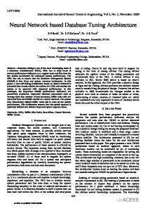
2.1 Biological Motivation The brain’s elementary building blocks are the neurons. The study of the neuron, its interconnections and its role in the information processing is one important research field in modern biology. The research on ANN starts by trying to simulate the function of a neuron. ANN researchers adopt a minimal cellular structure that can be seen in Figure 2.1 The dendrites are the transmission channels for the incoming information. The synapses are the contact regions with other cells and are responsible for supplying the dendrites with information. Some organs inside the cell body are responsible for keeping the cell continuously working. The mitochondria are responsible for supplying the cell with energy. The cell has one axon that is responsible for transmitting the output signal to other neurons. The information processing in the cell membrane is done via electrical signals produced by diffusion. In short, neurons transmit information using action potentials. The information processing involves a complex electrical combination and chemical process. The synapses control the direction of the information transmission. They can be inhibitory or excitatory depending on the kind of ion flowing through it. The cell processes information by integrating incoming signals. If the flow of ions (membrane potential) reaches a certain threshold, an action potential is generated at the axon of the cell. The information is not only transmitted but also weighed by the cell. Rojas (Rojas, 1996) explains that “signals combined in an excitatory or inhibitory way can be used to implement any desired logic function”. This explains the huge information processing capability of the neuron systems.



Axon

Myelin sheath Axon hillock Cell Body Nodes of Ranvier Nucleus Synapse

Dendrites

Figure 2.1 – General structure of a generic neuron (Freeman 1992)

Neuron information is stored at synapses. The synapses control the passage of ions, thus controlling the cell depolarization. The plasticity is the synaptic connection will determine the capacity of the cell in acting properly. Therefore, the synapses control is important information to the whole system’s functionality. In ANN this synaptic control efficiency is simulated via a constant that is multiplied to the flowing information on the input channels, the weight. The storage, processing and transmission of information at the neuron level are still not fully understood. Neurons form such complex nervous systems that researches in many areas such as mathematics, chemistry, medicine and psychology are trying to understand how cell nerves act. Computer science has played an important role on this research being an important test bed for the different concepts and ideas. Furthermore, ANN also can be seen as a computation paradigm that has much to be explored by scientists of computer science. For a deeper study on the biological foundations see Anderson, 1995 or Rojas, 1996.

2.1.1 The generic artificial neuron The term artificial neuron is used in the literature interchangeably with: node, unit, processing element or even computational unit. Depending on the author’s approach or goals, one of those will be used. Here the term neuron will be kept in order to maintain the



analogy to the biological structures when modeling the framework objects. But whenever necessary, neurons will be distinguished by using the terms natural or artificial. The artificial neuron is a pretty huge simplification of the natural neuron. It is important not to be too restrictive and not to try to make a one-to-one relationship between the natural and the artificial neurons. In this work there are no discussions about the simplifications done. There are no discussions whether the models are appropriate simplifications of the reality or not. This work is based on what is already accepted in the community, and tries to improve those concepts from a software-engineering point of view.

I nput S i g n al s

x1

W i1

x2

W i2

xn

yi S u m m in g J un ction

W in

Out pu t S i g n al

A ctivation F u n ct i o n

syn a p tic weights tim es input s ig na ls

Figure 2.2 – The artificial neuron

The artificial neuron has input and output channels and a cell body. The synapses are the contact points between the cell body and the input or output connections, having a weight associated to them. The artificial neuron can be divided into two parts: the first is a simple integrator of synaptic inputs weighed by connection strengths; the second is a function that operates on the output of the integrator. The result of the second function will be the neuron output. The artificial neuron is schematically drawn in Figure 2.2. There are several mechanisms for calculating the neuron output value, such as: linear combination, mean-variance connections and min-max connections (Simpson, 1992). The most common way of doing it is the linear combination where the dot product (inner product) of the input values with the connection weights is calculated. In general it is followed by a nonlinear operation, the activation function (also called neuron function). Next a detailed description of the linear combination is shown: 1. The ANN has several inputs (xj) and one output (yi).



2. Each input connection has an associated weight that controls the connection strength (wij) and is usually a real number. 3. The weights can be inhibitory or excitatory (typically negative and positive values). 4. The net input (Equation 2.1) is calculated by summing the input values multiplied by the corresponding weights (inner product or dot product). neti = ∑ x j wij j

Equation 2.1 - Calculating the net of the neuron

5. The output value (Equation 2.2) is calculated applying an activation function that uses the neti: yi = fi ( net i ) Equation 2.2 - Calculating the output of the neuron

Some possible activation functions are shown in the following section.

2.1.1.1

Activation function

There are many possible activation functions. The most common ones are: the Linear, the Step, the Ramp, the Sigmoid, and the Gaussian functions. The last four functions introduce nonlinearity in the network dynamics by bounding the output values within a fixed range.



f(x)

f(x)

β

θ x

x −δ (b)

(a) f(x)

f(x)

+γ x

-γ

x

(d)

(c) f(x) variance

x (e) Figure 2.3 – Activation functions (Simpson, 1992)

Linear Function The Linear function produces a linearly modulated output. It is described by Equation 2.3 and can be seen in Figure 2.3(a): f ( x ) = αx Equation 2.3 – Linear function

Where α is a positive scalar. Step Function The Step function produces only two values, β and -δ. If x is equal or exceeds a predefined value θ the function produces β, otherwise it produces -δ. The values β and δ are



positive scalars. This function is binary and is used in neural models such as the Hopfield (Hopfield, 1982) and the BAM (Kosko, 1988). The Step function is defined on Equation 2.4 and its result can be seen in Figure 2.3(b). β f ( x) =  − δ

if if

x ≥θ x 0 to shape the function. The Gaussian function definition is shown at Equation 2.7 and its effect can be seen in Figure 2.3(e).



f ( x) = exp(

− x2

υ

)

Equation 2.7 – Gaussian function

2.1.2 ANN Architectures The natural neurons form the neural nerves when connected. In ANN the artificial neurons are connected in many different ways forming architectural characteristics. The learning algorithms and the architectures are closely related. It is important to have a clear concept of how the artificial neurons may be interconnected to form the specific architectures, because this will define how the computer implementations of the architectures can be done. The possible computer implementation solutions for the specific architectures and learning algorithms are going to be explained later. Following the description of the principal ANN architectures is as follows.

2.1.2.1

Single-Layer Feedforward Networks

In this simplest network, a layer of input neurons is connected to a layer of output neurons. The “single-layer” designation refers to the output layer. The layer of input neurons is not considered because it does not process any computation over the input values. It just bypasses the input values. An example of this kind of neural network is a linear associative memory where an input pattern is associated to an output pattern, both in form of a vector. Figure 2.4 shows a single-layer network of 3 output nodes.

O u tp u t L a y e r Inp ut Layer

Figure 2.4 – Single-layer feedforward network

2.1.2.2 Multi-Layer Feedforward Networks In this architecture, one or more hidden layers of neurons are present. Those networks are able to deal with higher-order problems because of the extra set of connections and the extra dimension of neural iterations (Churchland and Sejnowski, 1992; Haykin, 1994).



Figure 2.5 shows a multi-layer 4-2-3 network that means a network formed by an input layer with 4 neurons, only one hidden layer with 2 neurons and an output layer with 3 neurons. The network is fully connected because each neuron in one layer is connected to all neurons in the next layer. It also may happen that not all the neurons of one layer are connected to all neurons of the subsequent layer. This may happen when the user has a certain previous knowledge about the pattern being classified. He/she is then able to preset the network connections. Figure 2.6 shows a multilayer 4-2-3 network not fully connected.

O ut pu t L a y e r

I n pu t L a y e r

Figure 2.5 – Multilayer feedforward network fully connected

O ut pu t L a y e r

I n pu t L a y e r

Figure 2.6 – Multilayer feedforward network not fully connected

2.1.2.3 Recurrent Networks This network model has at least one feedback loop. It may have the same architecture as a layered network, but it is necessary to have the feedback. The feedback can happen from the output of one neuron back to the input of another neuron. This feedback may happen among neurons of the same layer or neurons of different ones. The feedback may also happen as a self-feedback when the output of the neuron is returned to its own input. The feedback deeply influences the network learning capability and its performance. Figure 2.7



shows a single-layer recurrent network where the output signals of the neurons are fed to the input of the other neurons in the same layer.

O u tp u t L a y e r I np u t L a y e r

Figure 2.7 – Recurrent network with no self-feedback loops

2.1.2.4 Lattice Networks Lattice Networks consist of networks formed by arrays of neurons at any dimension. An input neuron is associated to each array supplying the signal to the array. Figure 2.8 shows a two-dimensional lattice network of 3-by-3 neurons fed from a layer of 3 input neurons. For each of the above architectures, various learning algorithms were proposed. In this work, the last 3 architectures were considered when choosing the test models once the singlelayer is a simplification of the multi-layer. Two multi-layer models were chosen, one case of fully connected network and one case of not fully connected network. The fully connected one is the Backpropagation (Rumelhard and McClelland, 1986) and the other one is the CNM (Machado and Rocha, 1990). The chosen recurrent network is the ART1 model (Grossberg, 1976; Grossberg, 1987) and the chosen lattice model is the SOM (Kohonen, 1982). The description of these 4 models is presented in Section 2.2 below.

Input L a y er

O utput L ayer Figure 2.8 – Lattice network



2.2 ANN Learning Algorithms Since the information of how the neurons process data is on the weights, the weight values will determine whether the neuron is able to accomplish a certain task or not. So learning is a process of finding weights that represent the system knowledge. In practice, the learning process is the modification of the weight values in order to make the output values the proper ones, given a certain input data. The learning law is determined by the modification of the strength of synaptic junctions based on a system of differential equations for the weight values. The system of equations is solved to an acceptable approximation solution. The values of the connection weights will determine how well the neural network solves the problems. These values may be predefined and hardwired into the network. However, such method is rarely adopted because it is very difficult to know in advance the appropriate values for the weights. A learning algorithm often determines the values of the weights. The learning algorithm is an automatic adaptive method that tries to fit the appropriate weights to the system solution. There is no explicit programming for the solution achieved. Several algorithms are available for changing the values of the connection weights. It is not the goal here to cover all the possible algorithms but to introduce the general ideas behind them. The learning algorithms are divided into two categories: supervised and unsupervised learning. Supervised learning is a process that incorporates global information and/or a teacher. The teacher regulates the learning, informs the network what it has to learn and checks if it has properly learned or not. Supervised learning has information deciding when to turn off the learning, deciding how long and how often to present each datum for learning, and supplying performance information. Some well-known algorithms that implement supervised learning are error correction learning, reinforcement learning and stochastic learning. Supervised learning can be subdivided into two subcategories: structural and temporal learning. The first tries to find the best input/output pattern relationship for each pattern pair. It is used to solve problems such as pattern classification and pattern matching. The second one is concerned with finding a sequence of patterns necessary to achieve some final



outcome. The current response of the network is dependent on the previous inputs and responses. Examples of use are prediction and control. The unsupervised learning uses only local information during the learning. It organizes presented data discovering their collective properties. Examples of unsupervised algorithms are Hebbian learning and competitive learning. In this work, there is no necessity to build up a complete taxonomy of the possible learning algorithms. There are several algorithms with innumerable variations. More complete lists of learning algorithms can be found in the neural networks literature such as Haykin, 1994; Simpson, 1992; and Rojas 1996. A brief explanation of some relevant supervised and unsupervised learning algorithms follows.

2.2.1 Hebbian Learning It is the simplest way of adjusting the connection weight values. It is based on the work of the neuropsychologist Donald O. Hebb (1949) (Haykin, 1994). Hebb hypothesized that the change in a synapse’s efficacy is prompted by a neuron’s ability to produce an output signal. It proposes a correlation-based adjustment of the connection weight values. That means if the activation of a neuron A repeatedly and persistently caused a neuron B to fire, then the efficacy of the connection among those neurons is improved. This idea was expanded to the inverse sense where either uncorrelated or negatively correlated activity produces synaptic weakening. The Hebbian synapses efficiency thus is a mechanism that is time dependent because it relies on the exact time of occurrence of the presynaptic and postsynaptic activities. It is also a highly local mechanism where the local available information is used to produce a local synaptic modification. Finally, the Hebbian synapse has an interactive nature because it depends on activities on both sides of the synapse, that is, it depends on the interaction among the presynaptic and postsynaptic activities. The mathematical models of Hebbian learning can be found in (Haykin, 1994; and Simpson, 1992). Important neural network models that implement this kind of learning include:



•

The Linear Associative Memory (Anderson, 1970; Kohonen, 1972; Haykin 1994) that employs this learning and analyzes its capabilities;

•

The Hopfield network (Hopfield, 1982) which is a one-layer network that restricts the neuron activity to either binary {0,1} or bipolar {-1,1} values and introduces feedback connections forming a nonlinear, dynamic system;

•

The Bidirectional Associative Memory (BAM) (Kosko, 1988), which implements this learning in a two-layer network.

2.2.2 Competitive Learning Competitive learning is a method of automatically creating classes for a set of input patterns. This kind of learning was introduced and extensively studied by Grossberg (Grossberg 1970, and 1982). The basic idea behind this learning method is that the output neurons compete among themselves for being the one to fire. Typically the input data is organized as vectors and the neural network maps the input vectors into its synaptic weights. The classes are represented by the groups of neurons that have the nearest synaptic vectors to a given input vector pattern. Important implementations of this kind of learning are:

•

The Adaptive Resonance Theory (ART) (Grossberg, 1987) where the neurons of the competitive layers shall compete to find appropriate pattern classifications without compromising the neural network capacities of generalization (stability) and discrimination (plasticity);

•

The Self-Organizing Feature Maps (SOM) also known as the Kohonen model (Kohonen, 1984) where neurons in the competitive layer compete to map the input features trying to simulate the cerebral cortex areas of storing the knowledge.

2.2.3 Error Correction Learning When applying a data value to the input layer of neurons of a neural network, this data value is processed by the network neurons sequentially until a signal reaches the output neurons of the network. The output values produced by the output neurons should be the desired output values. A learning algorithm can be used to gradually approximate the computed output to the desired output. The error correction learning adjusts the connection



weights considering the proportional difference between the desired and the computed values. A two-layer network implementing error correction learning is able to solve linear separable problems. Examples of two-layer neural networks that implement error correction learning are:

•

The Perceptron (Rosenblatt, 1962);

•

The ADALINE (Widrow and Hoff, 1960).

A multilayer network using error correction learning is able to capture nonlinear mappings between the input and output patterns. For a long time the problem was to establish an appropriate algorithm to do the error correction for the hidden neurons connection weights based on the output neurons output values. The point was to determine how dependent the network output is from the output generated by the hidden neurons. It is ultimately a problem of minimization of a cost-function based on the error signal produced by the network output. The solution is the use of partial differentiation to calculate weight changes for any weight in the network (the gradient descent method; Widrow and Stearns, 1985; Haykin 1994). An example of neural network using the multilayer error correction algorithm is:

•

The Backpropagation (Werbos, 1974; Parker, 1985; leCun, 1985; Rumelhart, Hinton and Williams, 1986), which introduced an error correction algorithm for multilayer networks.

2.2.4 Reinforcement Learning It is similar to error correction learning because the weights are also reinforced for correct performance, and punished for incorrect performance. The difference is that the error correction uses a more specific algorithm where the output of each neuron on the output layer is considered, while the reinforcement learning uses nonspecific error information to determine the performance of the network. Furthermore, in reinforcement learning the gradient descent is performed in probability space while in error correction learning is performed in error space. The reinforcement learning is ideal for using in prediction and control where there is no specific error information available, only overall performance information. Neural network examples that use reinforcement learning are:



•

The Adaptive Heuristic Critic neural network (Barto et al.,1983) which introduced the use of a critic to convert the primary reinforcement signal received from the environment into a higher-quality reinforcement signal called the heuristic reinforcement signal. The learning system consists of three components very much used in Artificial Intelligence: learning element, knowledge base and performance element. The learning element is responsible for doing all changes in the knowledge base, and the performance element is responsible for selecting actions randomly on the basis of a distribution that is determined by the knowledge base;

•

The Associative Reward-Penalty neural network (Barto, 1985).

2.2.5 Stochastic Learning This learning method adjusts connection weights to a multilayer network using random process, probability and energy relationship. The neural network escapes local energy minima in favor of a deeper energy minimum via probabilistic acceptance of energy states. The learning process is governed by a “temperature” parameter that slowly decreases the number of probabilistically accepted higher energy states. An example of this learning is:

•

The Boltzman machine (Ackley et al. 1985).

2.3 ANN Input and Output Data The neural network has to be set with data to do the learning and testing processes. All models need an input data pattern to be applied in its input neurons in order to learn or test this data pattern. The data to be applied to the network must be prepared in a way that the network is able to understand and process it. The quality of what is learned by the neural network depends very much on what the patterns are representing. Typically, each data pattern must be transformed in a vector of values that represent the pattern to be applied. The appropriate transformation of the data in the input vector is essential to the learning process. Many different features can be modeled from the same problem at hand. For example, the age of a person can be modeled as discrete values, sets, or fuzzy sets. Depending on how it was modeled, the network can succeed or not in the learning process. Furthermore, there are neural networks that need to have input and output patterns presented during the learning process, the networks based on supervised learning such as the



error correction learning algorithm. The input pattern is applied on the input neurons, then the signal flows over the network producing an output. The produced output is then compared with the desired output for the given input pattern. The comparison results in a difference that is used to do the error correction of the network connection weights. Some neural networks accept only binary data as input such as the discrete Hopfield model (Hopfield, 1982), other networks accept real numbers like the Backpropagation (Werbos, 1974; Parker, 1985; leCun, 1985; Rumelhart, Hinton and Williams, 1986). The number of neurons on the network input layer usually is determined by the size of the vector to be applied, so that each vector element value is applied to one input neuron. The number of neurons in the input and the output layers are not necessarily the same. The data preparation (pre-processing) for applying to the neural network simulation is a problem that has to be faced by the developer. A programmer often has to code the data transformation to the chosen ANN model, take care of the chosen ANN architecture (the number of neurons on the input and output layers) and so on. The hard coding of the data preparation can generate overhead in many situations:

•

For each new problem that the ANN has to be applied, a specific program has to be created to do the appropriate data pre-processing.

•

Frequently the ANN architecture is changed during the process of finding the appropriate solution because certain features are added, removed or applied in a different way.

•

Sometimes the solution via a neural model is not possible and the programmer chooses to go for another model. This may imply changing completely the way the data has to be pre-processed.

To avoid reprogramming of the data pre-processing in each of the above situations, it is important to use appropriate pre-processing tools that can easily integrate with the ANN implementation. One solution to have a nice integration is to create a pre-processing framework that deals with the data independently of the ANN model and the selected features. The construction of such a framework is proposed in this work via the Domain framework that is explained in Chapter 3.



2.4 Chosen ANN Models In the realm of this work, it is not possible to approach the various existing ANN models. Few models were picked up among the most important ones, based on some criteria such as: application interest (potential), architecture and kind of learning. The idea is to be able to cover a good variety of situations, being able to implement enough generalizations that could be useful for most of the ANN models without having to implement many models. The first chosen model was the Backpropagation (Werbos, 1974; Parker, 1985; leCun, 1985; Rumelhart, Hinton and Williams, 1986). This model implements a supervised learning based on the error correction learning algorithm. Its architecture is feedforward multilayer and it is fully connected. The Backpropagation is a widely used model for structural and temporal classifications. There are many variations of this model. The second chosen model is the Combinatorial Neural Model (CNM) (Machado and Rocha 1990). This model also implements supervised learning based on a variation of the error backpropagation learning algorithm. The network is feedforward and not fully connected. Besides being an important and interesting neural model by its concepts, the reasons to implement it in this work were twofold: the profound knowledge of the author on this model; and the special interest in the application of this model on the credit scoring problem of companies. Third, a typical unsupervised competitive learning model was chosen, the SelfOrganizing Feature Map (SOM) (Kohonen, 1984). The SOM architecture is based on a twodimensional lattice map. The SOM model has been largely applied in different areas such as image and speech recognition. Finally, another unsupervised competitive learning model was chosen, the Adaptive Resonance Theory (ART) (Grossberg, 1987). The extra important architectural aspect implemented by this model is the presence of feedback connections among its neurons, so the network has a recurrent architecture. Next, each of the four models is introduced. The goal here is not only to introduce the theoretical aspects of each model but also to find out the main characteristics of each one and, specially, the commonalties among the models. Those characteristics and commonalties are important to properly create an object model to build the neural network components.



2.4.1 The Backpropagation The Backpropagation neural network (Werbos, 1974; Parker, 1985; leCun, 1985; Rumelhart, Hinton and Williams, 1986) is a multilayer, feedforward network, using a supervised learning mode based on error corrections. Minsky and Papert (1969) have provided a very careful analysis of the capabilities of the neural models proposed so far. At that moment, the Perceptron was offered a very simple guaranteed learning rule (the delta rule – Widrow and Hoff, 1960) for all problems that can be solved by a two-layer feedforward network. What Minsky and Papert (1969) have shown was that this learning rule was capable of solving only linear separable problems. Later, Rumelhart, Hinton and Williams (1986) have shown that the addition of hidden neurons to the neural network architecture would permit the mapping of the problem representation in a way that nonlinear separable problems could be solved. The problem, at that moment, was that there was no specified learning rule to cope with the hidden neurons. The solutions that came up later to solve this problem were the following three:

•

The addition of weight values on the hidden neurons by hand, assuming some reasonable performance;

•

The competitive learning where unsupervised learning rules are applied in order to automatically develop the hidden neurons.

•

The creation of a learning procedure capable of learning an internal representation (using the hidden neurons) that is adequate for performing the task at hand.

The Generalized Delta Rule represents the latest approach, which implements a supervised learning algorithm based on the error correction in a multilayer neural network and which is known as the Backpropagation neural network. The proposed learning procedure involves the presentation of a set of input and output patterns to the neural network. The input patterns typically correspond to a sample of the real patterns. For each input pattern one output pattern is determined. The output patterns are the known classification of the correspondent input patterns. The patterns are represented in the form of a vector. When learning, the system first uses the input vector to produce its own output vector and then compares this with the desired output (the output pattern). If there is no



difference, no learning takes place, but if there is a difference, the weights of the network are changed in order to reduce this difference. The generalized delta rule minimizes the squares of the differences between the actual and the desired output values summed over the output neurons and all pairs of input/output vectors. There are many ways of deriving the delta rule; derivations are detailed in (Rumelhart at al.1986). Figure 2.9 shows a generic Backpropagation neural network architecture with one layer of hidden neurons. The network is fully connected, having all neurons of one layer connected to all neurons of the next layer. It has an input layer which number of neurons corresponds to the size of the input vector. The number of neurons for the output layer corresponds to the size of the output vector. The Backpropagation may have more than one layer of hidden neurons. The number of neurons on the hidden layer may define the capability of the network in mapping the problem properly. Usually the determination of the number of neurons on the hidden layers and the number of hidden layers is very difficult. Typically, the network developer or user determines them empirically. Output Patterns

...

...

...

...

Output Layer

Hidden Layer

Input Layer

Input Patterns Figure 2.9 – Generic Backpropagation network

Next, a sequence of equations will be introduced showing the mathematical description of the generalized delta rule or the Backpropagation algorithm.



First the input vector xp = (xp1, xp2,…, xpN)t is applied to the input layer of the network. The input neurons just bypass the input values to the hidden neurons via the connection synapses. The hidden neurons will calculate its net using Equation 2.8: N

net pj = ∑ w ji x pi + θ j i =1

Equation 2.8 – Hidden neurons net

In Equation 2.8, p is the pattern being learned, j denotes the jth hidden unit, w ji is the weight on the connection from the ith input unit to the jth hidden unit, and θ j is the bias value. The bias is useful to accelerate the network convergence. Equation 2.9 gives the activation of the hidden neuron.

i pj = f j (net pj ) Equation 2.9 – Hidden neurons activation

The calculation of the output neurons net (netpk) and the corresponding output value (Opk) is the same as shown in Equations 2.10 and 2.11. In these equations, the difference to Equations 2.8 and 2.9 is that the index k denotes the kth output unit. N

net pk = ∑ wkj i pj + θ k j =1

Equation 2.10 – Hidden neurons net

o pk = f k (net pk ) Equation 2.11 – Hidden neurons activation

Function f can assume several forms as seen previously on the activation functions exemplified in Figure 2.3 (Activation functions). Typically, two forms are of interest: linear and sigmoid output functions given by Equations 2.12 and 2.13 respectively. The same function forms are valid for both hidden and output neurons.

f k (net pk ) = net pk Equation 2.12 – Linear output function



f k (net pk ) = (1 + e

− net pk

) −1

Equation 2.13 – Sigmoid output function

After propagating the input signals over the network as explained by the equations above, it is time to calculate the local gradients for the output and hidden layers. This calculation is done based on the difference between the real and the desired output, that is the principle of the supervised learning as already explained. The calculation of the local gradients for the hidden neurons is done before the update of the connection weights to the output layer neurons. Equation 2.14 shows the calculation of the local gradients for the output neurons.

δ pk = ( y pk − o pk ) f k´ (net pk ) Equation 2.14 – Output neurons local gradients function

Equation 2.15 shows the calculation of the local gradients for the hidden neurons.

δ pj = f j´ (net pj )∑ δ pk wkj k

Equation 2.15 – Hidden neurons local gradients function

Equation 2.16 shows the f´ function that is the derivative of the sigmoid activation function in respect to its total input, netpk. The function shown is the one used for the output neurons, the same is valid for the hidden neurons changing the index k by index j.

f k´ (o pk ) = o pk (1 − o pk ) Equation 2.16 – Sigmoid function derivative

Having calculated the local gradients for all neurons on the output and hidden layers, it is time to go backwards recalculating the weights of the neural network based on those local gradients. It is necessary to calculate the negative of the gradient of Ep (error for the example pattern p), ∇E p , with respect to the weights wkj, to determine the direction in which to change the weights. Then the weights are adjusted so that the total error is reduced. Equation 2.17 calculates the error term Ep that is useful to determine how well the network is learning. When the error is acceptably small for each of the training examples, the training can be



stopped. Figure 2.10 exemplifies a hypothetical error surface in weight space, its local and global minima and the gradient descendent. Ep =

1 M 2 ∑ δ pk 2 k =1

Equation 2.17 – Error term

Ep Ep Z Ep

Zmin Figure 2.10 – Hypothetical error surface

The constant that assures the proportionality of the error adjustments steps is the learning rate η . The larger this constant, the larger the changes in the weights. The chosen learning rate shall be as large as possible without leading to oscillation. One way to avoid oscillation is to include to the generalized delta rule a momentum term that has a parameter

α . Thereby Equation 2.18 gives the weight change for the connections among the output and hidden neurons in the iteration time t. ∆ p wkj (t ) = η (δ pk i pj ) + α∆ p wkj (t − 1) Equation 2.18 – Weight change magnitude for connections among output and hidden neurons

Equation 2.19 gives the update of the weight value for the connections among the output neurons and the hidden neurons. wkj (t + 1) = wkj (t ) + η (δ pk i pj ) + α∆ p wkj (t − 1) Equation 2.19 – Weight update for connections among output and hidden neurons



Similarly, Equation 2.20 gives the weight change for the connections among the hidden and the input neurons in the iteration time t. ∆ p w ji (t ) = η (δ pj xi ) + α∆ p w ji (t − 1) Equation 2.20 – Weight change magnitude for connections among hidden and input neurons

Then Equation 2.21 gives the update of the weight value for the connections among the hidden neurons and the input neurons. w ji (t + 1) = w ji (t ) + η (δ pj xi ) + α∆ p w ji (t − 1) Equation 2.21 – Weight update for connections among hidden and input neurons

Once the network learning reaches a minimum, either local or global, the learning stops. If it reaches a local minimum, the error produced at the network outputs can still be unacceptably high. The solution then is to restart the network learning from scratch with new weights for the connections. If this is still not the solution, the number of neurons on the hidden layer can be improved, or the learning parameters learning rate and momentum can be changed. Important aspects to consider on the object model for the Backpropagation are:

•

The input nodes just bypass the information. Usually this information is a normalized set of values between 0 and 1, resulting from a pre-processing of the input data.

•

The hidden and the output neurons implement the Perceptron functionality where the dot product is applied and a nonlinear function gives the neuron activation.

•

In the original model the connections among the neurons are feedforward. There are no feedback connections and the network is fully connected.

•

The number of input, hidden and output neurons is determined based on the expert knowledge on the application domain.

•

Even not having feedback connections the backward propagation of the error terms is a computation in the reverse direction. In fact, the backward



computation is as important as the forward computation on this model, being an important and interesting characteristic to be modeled. The given Backpropagation equations presented here are from Freeman, 1992.

2.4.2 The Combinatorial Neural Model The Combinatorial Neural Model (Machado and Rocha 1989, 1992; Machado et al. 1998) has been explored and developed during the past decade. Experiments with this model have demonstrated that it is well suited for classification problems, with excellent results in terms of accuracy (Leão and Rocha 1990; Feldens and Castilho 1997). The CNM integrates, in a straightforward architecture, symbolic and non-symbolic knowledge. This model has characteristics that are desirable in a classification system:

•

Simplicity of neural learning - due to the neural network’s generalization capacity.

•

Explanation capacity – the model can map a neural network’s knowledge into a symbolic representation.

•

High-speed training - only one pass over the training examples is required.

•

Immunity against some common neural network’s pitfalls – i.e. local optima, plateau, etc.

•

Incremental learning possibility - previously learned knowledge can be improved with new cases.

•

Flexible uncertainty handling – it can accept fuzzy inputs, probabilistic inputs, etc, as inputs fall into the interval [0, 1].

The CNM includes mapping of previous knowledge to the neural network, training algorithms, and pruning criteria, in order to extract only significant pieces of knowledge. The detailed explanations on the possible learning algorithms are in (Machado et al. 1998). Here are considered the Starter Reward and Punishment (SRP) and the Incremental Reward and Punishment (IRP) learning algorithms, which are the original learning algorithms proposed for the model. Those learning algorithms offer the possibility of building a CNM network based



on knowledge elicited from an expert (using SRP), and the possibility of refinement with new examples the knowledge existing in the network (using IRP). Output Neurons (hypotheses)

? Input Neurons (findings) Learning Algorithm

Output Neurons (hypotheses)

Combinatorial Neurons

Input Neurons (findings)

Figure 2.11 – The CNM network generation

The CNM is a 1-hidden layer, feed-forward network. It has particular characteristics in the way the topology is constructed, in neurons, in the connections among neurons, and in its training algorithm. The domain knowledge is mapped to the network through evidences and hypotheses (Figure 2.11). The evidence may have many distinct values that must be evaluated separately by the neural network, called findings. The input layer represents the defined set of findings (also called literals). A finding can be a categorical or numeric pattern feature. The categorical feature can only take on a finite number of values while a numeric feature may take on any value from a certain real domain. A categorical feature requires at most one input neuron for each of the feature possible values. The state of each such neuron is either zero or one. A numeric feature has to be partitioned in fuzzy sets where each set will correspond to an input neuron and its state will correspond to the fuzzy set degree of membership. An example: if an evidence age is modeled, it probably has findings that can be modeled as fuzzy intervals (Kosko, 1992). The domain expert defines fuzzy sets for different ages (e.g. child, adolescent, adult, senior) (Figure 2.12). Each fuzzy set defined will correspond to a finding and, as a consequence, to a CNM input neuron.



1 Fuzzy Value 0.6 0.3 0

child

youth 16

12

adult 19

senior 50

Fuzzy Set

Figure 2.12 - Fuzzy Sets

In this case each input value is in the [0,1] interval (fuzzy set membership functions), indicating the pertinence of the training example to a certain concept, or the degree of confidence. In the example of Figure 2.12, the age 19 will correspond to a zero membership value for the child and senior fuzzy sets and to a 0.6 value for the adolescent fuzzy set and 0.3 to the adult fuzzy set. The intermediate (combinatorial) layer is automatically generated. A neuron is added to this layer for each possible combination of evidences, from order 1 to a maximum order, given by the user. The output layer corresponds to the possible classes (hypotheses) to which an example could belong. Combinatorial neurons behave as conjunctions of findings that lead to a certain class. For that reason, the pth combinatorial neuron propagates input values according to a fuzzy AND operator (Equation 2.22), taking as its output the minimum value received by the inputs. min sip ( xi )

i ∈ Ip

Equation 2.22 – Fuzzy AND

In Equation 2.22 above, I p ⊆ {1,..., n} indicates the appropriate input neurons, and either sip ( xi ) = xi or sip ( xi ) = 1 − xi (fuzzy negation). In the first case the synapse (i,p) is called excitatory and in the later case inhibitory. Output neurons group the classification hypotheses implementing a fuzzy OR operator (Equation 2.23), propagating the maximum value received by its inputs.



max w p min sip ( xi ) 1≤ p ≤ m

i ∈ Ip

Equation 2.23 – Fuzzy OR

In Equation 2.23 above, m indicates the number of output neurons, and w p ∈ [0,1] is the weight associated with the connection from the pth combinatorial neuron to the output neuron. The weights modifications are determined by using a supervised algorithm which attempts to minimize the mean square error (Equation 2.24) incurred by the network when presented with a set of examples.

mse( w) =

1 [ y (e, w) − yˆ (e)] 2 ∑ E e∈E

Equation 2.24 – Mean Square Error calculation for the new weight set of values

In Equation 2.24 above, w is the weight vector of a CNM network, and the learning is done using a set of examples E ⊂ [0,1] n . For an example e ∈ E , let yˆ (e) denote the desired output, and y(e,w) the output generated by the network with the weight vector w. The Incremental Reward and Punishment (IRP) and the Starter Reward and Punishment (SRP) learning algorithms are based on the concept of rewards and punishments. The connections between neurons (synapses) have weights and also pairs of accumulators for punishment (Pp) and reward (Rp). Before the training process, in absence of previous knowledge, all weights are set to one and all accumulators to zero. During the training, as each example is presented and propagated, all links that led to the proper classification have their reward accumulators incremented. Similarly, misclassifications increment the punishment accumulators of the path that led to wrong outputs. Weights remain unchanged during the training process, only accumulators are incremented. The training process is generally done in one pass over the training examples. At the end of this sequential pass, the connections that had more punishments than rewards are pruned. The remaining connections have their weights changed using the accumulators.


2.4.2.1


The IRP learning

The IRP is used when the CNM neural network already exists and the goal is to add new knowledge to the network by learning new examples. In the case of the IRP, the learning proceeds as following. If for a weight vector w, an example e ∈ E yields y(e,w) > yˆ (e) , then every pathway p (connection among a combinatorial neuron and an output neuron), in the network is rewarded proportionally to:

•

The response of the network, y(e,w);

•

The absolute value of the error, y (e, w) − yˆ (e) ;

•

The signal injected by p into the output neuron, w p min s ip ( xi (e)) . i ∈ Ip

On the other hand, when y(e,w) < yˆ (e) each pathway of the network is punished in the same way. At the end of each learning iteration, the synapses with the Rp < Pp are deleted (pruned), and for the others, the accumulators are used to recalculate the value of wp. The remaining pathways with Rp > 0 and Pp = 0 (pathognomonic pathways) have their weights updated based on Equation 2.25: w p = t + (1 − t )

Rp max ( Rq − Pq ) 1≤ q ≤ m

Equation 2.25 – Pathognomonic pathway weight update

The constant t is an arbitrary acceptance threshold and t ∈ (0,1] . The other remaining pathways (ordinary pathways), have their weights updated based on Equation 2.26: wp =

R p − Pp max ( Rq − Pq ) 1≤ q ≤ m

Equation 2.26 – Ordinary pathway weight update



At the end of the iteration, the values of Rp and Pp are passed on to the next iteration, enabling the incremental learning capability. 2.4.2.2

The SRP learning

The SRP learning applies the same general principle of rewards and punishments of the IRP learning in a one-iteration procedure. Before applying the SRP, the accumulators are set to zero and the weights are set to one. All the data examples are then applied to the network in a one-iteration procedure promoting the changes of the reward and punishment accumulators. After applying all examples, the same weight updates used on IRP are applied: the non-rewarded pathways are pruned and the others have their weights modified by Equations 2.25 and 2.26 above. The SRP is the starting point for the CNM learning. After its application, the IRP can be used to increment the CNM knowledge. Important aspects to consider on the object model for the CNM are:

•

The input neurons just bypass the information. Usually this information is normalized values among 0 and 1, resulting from a pre-processing of the input data.

•

The combinatorial neurons implement the fuzzy AND function and the output neurons operate the fuzzy OR function.

•

The connections among the neurons are feedforward, there are no feedback connections and the network is not fully connected.

•

The number of input and output neurons is determined based on the domain knowledge the expert has, and the combinatorial neurons are created as the possible combinations, from zero to a given order number (typically 3), of the input neurons. The generation of the combinatorial layer may demand enormous memory footprint to be able to generate the neurons and synapses to all necessary combinations.

•

The CNM synapses have reward and punishment accumulators that are used to decide whether the synapse must be pruned or not, and also to recalculate the new value for the synaptic weight.



2.4.3 The Self-Organizing Feature Maps This kind of neural network is inspired on the brain’s cortical structure. The different sensory inputs like visual or acoustic are mapped in different areas of the cerebral cortex in a topologically ordered manner. The Kohonen Self-Organizing Feature Map (SOM) (Kohonen, 1990) was built to operate in an analog way. The network is based on a usually twodimensional lattice structure. The learning is competitive where the neurons are selectively tuned to various input patterns (vectors) or classes. The different input features force the locations of the winning neurons to be ordered in respect to each other in a meaningful way, so that the different features are mapped to different regions of the lattice. The spatial locations of the neurons correspond to the features given in the input patterns. An important characteristic of the SOM neural network is the presence of lateral feedback in the learning process. The lateral feedback is a special form of feedback that is dependent on lateral distance from the point of its application. The lattice network has “imaginary” lateral connections among the neurons. The neuron on the map that best fits the feature of the pattern being presented to the network is considered the network winner. The neurons that are located around the winner neuron shall receive excitatory or inhibitory effects depending on the distance of the winner neuron through the lateral connections. This effect is due to the called bubble activity the network tends to have by concentrating the electrical activity into local clusters. Exciting or inhibiting the neurons around the winner forms the feature clusters. Typically the Gaussian function shown in Figure 2.3(e) (Activation functions) is used to describe the lateral feedback. The Kohonen SOM neural model basic functionality can be described as follows:

•

The input of the network can be of any dimensionality while a one or twodimensional lattice of neurons is responsible for computing simple discriminant functions of the input.

•

A mechanism compares these discriminant functions and selects the neuron with the largest discriminant function value.

•

The selected neuron and its neighbors are activated simultaneously.

•

An adaptive function increases the discriminant function values of the selected neurons in relation to the input signal.



The Kohonen SOM neural network structure can be seen in Figure 2.8 (Lattice network) that shows the lattice architecture or in Figure 2.13 below. Figure 2.13 tries to show that the SOM network is fully connected, all neurons on the input layer are connected to all neurons on the output (lattice) layer. It shows also the connections among the neurons on the output layer that will be responsible for the lateral feedback. The number of input neurons is determined by the size of the input vector. The input vector represents the data pattern and can be of any dimensionality. The output map of neurons may have the dimensionality augmented to three, but the two-dimensional map is the most frequently used. The first step on the SOM learning is to find the winner neuron or the neuron that best matches a certain criterion. The winner neuron will determine the location of the activation bubble on the map. The network connections are initialized with random values so that no representation is given on the map at the beginning.

Two-dimensional lattice of output neurons ...

...

...

...

...

Connections among input and output neurons Input neurons

Figure 2.13 – Kohonen SOM

When the input pattern is applied to the SOM input, the values are propagated to all neurons on the lattice layer. The lattice layer can compute the arriving input signals by simply calculating the inner product to all output neurons. Considering that the threshold is the same for all the output neurons, the output neuron that produces the largest inner product is the one that best fits to the pattern and is selected as the winner. A second form of bestmatching is to use the minimum Euclidean distance between the vectors formed by the input signal and the weights at the arriving connections of each output neuron. In this case, the input vector and the network weights shall be normalized to constant Euclidean norm



(length). Equation 2.27 shows how to calculate the winner neuron i for a given input vector x using the minimum Euclidean distance. i ( x) = arg j min x − w j Equation 2.27 – Winner neuron calculation using the minimum Euclidean distance

In Equation 2.27 above, x is the learning vector and wj is the vector formed by the connections weights among the input nodes and the output neuron with index j. The Euclidean distance for a given output neuron with index j can be given by Equation 2.28 below, where p is the number of input neurons, wj,i is the weight of the connection among the jth output neurons and the ith input neuron, and xi is the input value applied to the ith input neuron.

x − wj =

p

∑ (x i =1

i

− w j ,i ) 2

Equation 2.28 – Euclidean distance

The topology of the lattice determines the neurons that are the neighbors of the winner neuron i. The weights of the connections to the winner neuron are to be rewarded by being this neuron the best matching to the given input. The neighbor neurons also shall receive some sort of reward forming the activation bubble together with the winner. By the lateral feedback connections, the neighbor neurons will be adapted to the given input. Let the lateral distance of the neuron j from the winning neuron i be denoted by dj,i. The amplitude of the topological neighborhood centered on the winner neuron i is denoted by π j ,i . Typically the neighborhood function is given by the Gaussian-type function shown in Equation 2.29.

π j ,i

 d 2j ,i   = exp −  2σ 2   

Equation 2.29 – Gaussian-type function for the topological neighborhood

The parameter σ at Equation 2.29 is the efective width (variance) of the topological neighborhood. The topological neighborhood π j ,i is maximum at the winning neuron (dj,i =



0). The amplitude of the topological neighborhood decreases with increasing lateral distance dj,i , decaying to zero for d j ,i → ∞ . The update of the synaptic weight vector wj of neuron j at lateral distance dj,i from the winning neuron i(x) is given by Equation 2.30 below, where n denotes the discrete time and η is the learning-rate parameter of the algorithm. w j (n + 1) = w j (n) + η (n)π j ,i ( x ) (n)[ x(n) − w j (n)] Equation 2.30 – Weight update function

The time-dependent learning-rate parameter η(n) used to update the synaptic weight vector wj(n) shall be time-varying. During the first 1000 iterations it shall assume a value near to the unity and be decreased gradually until a value above 0.1. The width of the topological neighborhood σ(n) shall also decrease slowly during the learning process. Typically, the function used for the calculation of both parameters is the exponential decay, described at Equations 2.31 and 2.32.

n  τ  1 

η (n) = η 0 exp −

Equation 2.31 – Learning-rate parameter update

n  τ  2 

σ (n) = σ 0 exp −

Equation 2.32 – Topological neighborhood parameter update

In Equations 2.31 and 2.32 above, the values σ0 and η0 are respective values of σ(n) and η(n) at the initiation of the algorithm (n=0). The values τ1 and τ2 are the time constants for the parameters η and σ respectively. Equations 2.31 and 2.32 shall be used only during the ordering phase, the first 1000 iterations or so, after that a small value shall be used for many iterations. Important aspects to consider on the object model for the SOM are:



•

The input nodes just bypass the information. Usually this information is normalized values among 0 and 1, resulting from a pre-processing of the input data.

•

The output neurons implement the Euclidean distance to find out its activation value.

•

The connections among the neurons of the input and output layers are feedforward and fully connected, there are feedback connections among the neurons of the output layer. The lateral feedback is a novel characteristic in relation to the previous models seen so far. There is no hidden layer.

•

The number of input neurons is determined by the expert based on the domain to apply the model. The number of output neurons is also determined empirically and is typically a two-dimensional map.

•

The activation bubbles form the chunks of knowledge about the problem being treated by the network. Each chunk tends to map an input feature.

The given SOM equations presented here are from the Haykin, 1994.

2.4.4 The Adaptive Resonance Theory The Adaptive Resonance Theory (ART) was proposed by (Grossberg, 1976; Grossberg, 1987). When proposing the ART model, Grossberg attempted to solve what he called the stability-plasticity dilemma. This dilemma is concerned with the neural network capacities of generalization (stability) and discrimination (plasticity). The stability property is responsible for the neural network capability of grouping similar patterns in the same category. The plasticity is the network capacity of creating new categories when new patterns are presented. The dilemma lives in the difficulty of having a neural model that is able to develop the two capabilities at the same time. It means the network shall: remain adaptive (plastic) in response to relevant input, yet remain stable in response to irrelevant input; know to switch between its plastic and its stable modes; retain its previously learned information while continuing to learn new information. Regarding the stability and plasticity properties of the ART model Grossberg stated: “An ART system can adaptively switch between its stable and plastic modes. It is capable of plasticity in order to learn about significant new events, yet it can also remain stable in



response to irrelevant events. In order to make this distinction an ART system is sensitive to novelty. It is capable, without a teacher, of distinguishing between familiar and unfamiliar events, as well as between expected and unexpected events.” (Grossberg, 1987) Grossberg introduced a feedback mechanism between the competitive and the input layers of the network to cope with the stability-plasticity dilemma. This feedback mechanism controls the learning in a way that new information is learned without destroying old information. Several models were derived from the Adaptive Resonance Theory (Grossberg, 1987; Carpenter and Grossberg, 1987; Carpenter and Grossberg, 1992):

•

ART1 – Is characterized by using only binary input.

•

ART2 – Is able to process analog input.

•

ART3 – Considers the action of the neurotransmitters on its synaptic mechanisms.

•

Fuzzy ART – Implements fuzzy concepts in ART1 architecture.

•

ARTMAP – Predictive architecture based on two ART modules.

•

Fuzzy ARTMAP - Predictive architecture based on two Fuzzy ART modules.

The name “resonant” on the model comes from physics where the resonance occurs when a small-amplitude vibration of the proper frequency causes a large-amplitude vibration in a mechanical or electrical system. In the ART network, the signals reverberate back and forth between neurons of the input and competitive layers. In this process, the network tries to stabilize by developing the proper pattern. If it does so, a stable oscillation ensues, which is the neural network equivalent of resonance. During the resonant period the learning or adaptation occurs. Before the network has achieved the resonant state no learning occurs. If a completely new pattern is presented to the ART network, it first tries to find on its internal representations the matching for the pattern. If the network does not find one, it enters in a resonant state in order to develop a new internal representation for the pattern. If the network has previously learned to recognize a pattern, then it will quickly enter in resonance and will reinforce the previously created internal representation.



In the ART model, two subsystems interact in the processing of the input patterns: the attention subsystem and the orientation subsystem. The attention subsystem is responsible for the processing of familiar input patterns, establishing responses and precise internal representations for those patterns. The orientation subsystem copes with the unknown patterns, resetting the attention subsystem when such patterns are presented to the network. An important role performed by the ART systems is to distinguish in a certain set of patterns what is signal and what is noise. To turn this possible, the context of the patterns was considered on the ART definition. Certain characteristics can be considered as noise when presented in certain patterns and considered as important signal feature for other patterns. The relevant information that shall be distinguished is called critical feature patterns, or prototypes and represent invariants of the set of all experienced input patterns. As the learning process takes place, new equilibrium points are formed as the system discovers and learns the critical features. The learned features are stabilized by internal mechanisms that internally control the learned features and avoid possible sources of system instability. Next, one model was picked from the ART family to be implemented in this work. The fourth model to be implemented is the ART1. The implementation of this ART model shall prove the capacity of the designed ANN framework to cope with feedback connections. Having this first ART model implemented, it is then easier to go for the implementation of the several other models of the ART family.

2.4.4.1 The ART1 In the ART architecture (Figure 2.14), two distinct processes occur when an input pattern is applied. The bottom-up process, also known as the adaptive filter or process of contrast enhancement, that produces the Y pattern, and the top-down process, that realizes a similarity operation to produce the pattern X*. Given a set of input patterns, a certain pattern belonging to this set is represented by I. When pattern I enters F1 (attention subsystem), it is then called pattern X (I and X are then identical). The neurons activated by the pattern X in F1 generate output signals that flow through the connections F1→ F2 (long-term-memory). This process produces pattern Y on layer F2. This pattern Y is the result of a winner-take-all process where only one neuron in F2 can be the winner (the one with bigger activation). Only the winner neuron produces the value 1 on its output, the other neurons on the same layer produce 0. Here the bottom-up process finishes and the top-down process starts.



Attention Subsystem

Orientation Subsystem F2

STM +

+

... Y/Y*

-

T +

U

+

LTM +

V

S

X* +

F1

STM

+

-

... X +

+

+

Input Pattern I

Figure 2.14 – ART1 Architecture

From the winner neuron a top-down pattern is produced through the F2→ F1 connections (feedback connections). This new signal is called pattern V. Now, there are two stimulation sources for the input layer F1: the input pattern I and the feedback pattern V. Together they give origin on F1 to pattern X* that is typically different from pattern X. Pattern X* indicates the similarity level between the input pattern and the stored prototype on the connection among layers F2 and F1. The similarity process among those patterns can be simply the function AND (∩), or another similarity measure. It is then necessary to decide whether the input pattern must be stabilized on the winner neuron or another neuron should be used. To verify the level of similarity represented on X* it is necessary to define a rule that considers both X* and I. It is possible to consider several different rules for accepting or rejecting the stabilization. This rule is called the reset rule and Inequality 2.33 commonly defines it.

V ∩I I

=

X* I

≥ρ

Inequality 2.33 – Reset rule



In the Inequality 2.33, ρ is the vigilance parameter that can assume values between 0 and 1, |X*| is the number of ones in the pattern X*, and | I | is the number of ones in the pattern I. If the result of this equation is true, the winner neuron is considered stable. Otherwise, it will not be considered by the orientation subsystem A, and the search for a stable pattern will continue. If no neuron is accepted as stable, then a neuron that is not used to any input pattern is then selected to learn this new input pattern. After choosing a stable pattern, the network learns the input pattern by adaptation of the bottom-up and top-down connections. The 2/3 rule Figure 2.15 shows the application of the 2/3 rule. There are situations when the neurons on the F1 layer must be deactivated, i.e., not producing output signals. For example, the neurons on F1 do not have to generate outputs when excited only by the pattern V, but must be able to generate output when excited by the input pattern I. A mechanism called gain control (B) is implemented on the network to control such a situation. When F2 is active, excitatory signals to F1 are generated (pattern be V) and at the same time the gain control is inhibited (Figure 2.15(a)). The rule that controls layer F1 is called 2/3 rule and says that: two of the three signal sources available in F1 (input pattern I, top-down pattern V, and the gain control pattern B), are necessary to activate the F1 layer neurons producing an output pattern. These outputs from the neurons on the F1 layer are called supraliminal signals. During the button-up process, F1 receives an input that is the pattern I and an excitatory signal from the gain control, turning possible then the generation of the supraliminal signals (Figure 2.15(b)). During the similarity process of the top-down and bottom-up patterns, also supraliminal signals are generated (Figure 2.15(c)). Neurons that receive one bottom-up or one top-down input, not both, cannot generate the supraliminal signals.



F2 + B

F2 (a)

(b)

F1

B

+ +

F1 +

F2 +

(c)

F1

B +

+

Figure 2.15 – The 2/3 rule

Learning on ART1 There are two ways of doing the learning on ART1: the slow and the fast learning. The slow learning allows for only a small amount of the input pattern to be represented by the weights. After repetitive presentations of the entire set of learning examples, the most important features of each pattern are captured by the LTM (long term memory). This form of learning is well suited to problems with high dimensionality, subject to learning sets with huge amounts of noise. The fast learning quickly encodes the input pattern features on the weights. This encoding typically is done in a one-shot-learning, which means, each input pattern of the learning set is presented to the network only once and the network is able to learn the pattern features. The fast learning is recommended to learning sets free of noise and when the learning must be done immediately. Slow learning

The equations for the slow learning at the LTM and the STM (short-term-memory) described in (Carpenter and Grossberg, 1887) are as follows:

STM Equations



Equation 2.34 gives dynamic equation for calculating the activation of the STM xk of any neuron vk in F1 and F2.

ε

d x k = − x k + (1 − Ax k ) J k+ − ( B + Cx k ) J k− dt Equation 2.34 – STM activation

In Equation 2.34 above, J k+ is the total excitatory input to vk , J k− is the total inhibitory input to vk , and all parameters are positive. Parameter A controls the bottom-up and topdown signals, while B and C regulate the gain control. If A > 0 and C > 0, then the STM activity xk(t) remains within the finite interval [-BC-1, A-1], regardless of the values of J k+ and J k− .

The neurons on F1 are called vi, where i = 1,2,…M. The F2 neurons are called vj, where j = M+1,M+2,…N. Thus Equation 2.34 above turns to be Equation 2.35 below for the neurons on the F1:

ε

d xi = − xi + (1 − A1 xi ) J i+ − ( B1 + C1 xi ) J i− dt Equation 2.35 – STM for neurons on the F1

Similarly, Equation 2.34 above turns to be Equation 2.36 below for the neurons on the F2:

ε

d x j = − x j + (1 − A2 x j ) J +j − ( B2 + C 2 x j ) J −j dt Equation 2.36 – STM for neurons on the F2

For a discrete calculation of F1 an input vector Ii is applied and the activities are calculated according to Equation 2.37 below: x1i =

Ii 1 + A1 ( I i + B1 ) + C1

Equation 2.37 – Activities for the neurons on the F1



The J k+ input of the ith neuron vi in F1 is a sum of the bottom-up input Ii and the topdown input pattern Vi , represented by Equation 2.38 below: J i+ = I i + Vi Equation 2.38 – F1 input

The top-down input pattern Vi is given by Equation 2.39 below: Vi = D1 ∑ f ( x j ) z ji j

Equation 2.39 – Top-down input pattern Vi

The f(x) on Equation 2.38 above is the signal generated by activity xj of vj , and zji is the LTM trace in the top-down connection from vj of vi . In the notation of Figure 2.14 (ART1 Architecture), the input pattern I = (I1, I2,…,IM), the signal pattern U = (f(xM+1), f(xM+2),…, f(xN)), and the template pattern V = (V1,V2,…,VM). The inhibitory input J i− governs the attentional gain control signal and is calculated by Equation 2.40: J i− = ∑ f ( x j ) j

Equation 2.40 – F1 attentional gain control

Thus J i− = 0 if and only if F2 is inactive. When F2 is active, J i− > 0 and hence term J i− in Equation 2.35 (STM for neurons on the F1) has a nonspecific inhibitory effect on all

the STM activities xj of F1. The inputs and parameters of STM activities in F2 are chosen so that the F2 neuron that receives the largest input from F1 wins the competition for the STM activity (winner-take-all). The inputs J +j and J −j to the F2 neuron vj have the form given in Equations 2.41 and 2.42 respectively:

J +j = g ( x j ) + T j Equation 2.41 – F2 input



J −j = ∑ g ( x k ) k≠ j

Equation 2.42 – F2 attentional gain control

Input J +j adds a positive feedback signal g(xj) from vj to itself to the bottom-up adaptive filter input Tj given by Equation 2.43 below:

T j = D2 ∑ h( xi ) z ij i

Equation 2.43 – Bottom-up adaptive filter input Tj

The h(xj) is the signal emitted by the F1 neuron vi and zij is the LTM trace in the connection from vi to vj . Input J −j adds up negative feedback signals g(xk) from all the other nodes in F2. In the notation of Figure 2.14 (ART1 Architecture), the output pattern S = (h(x1), h(x2),…, h(xM)), and the input pattern T = (TM+1 ,TM+2,…, TN).

LTM Equations The LTM value for the bottom-up connection from vi and vj follows Equation 2.44: d z ij = K 1 f ( x j )[h( xi ) − Eij z ij ] dt Equation 2.44 – LTM for bottom-up connections

Similarly, the LTM value for the top-down connection from vj and vi follows Equation 2.45: d z ji = K 2 f ( x j )[ h( x i ) − E ji z ji ] dt Equation 2.45 – LTM for top-down connections

On Equations 2.44 and 2.45 above, K1 and K2 are positive constants that control the learning rate, Eij and Eji are positive constants that control the decay rule (see Carpenter and



Grossberg, 1987), zij is the value for the connection from vj to vj , and zji is the value for the connection from vj to vi. The threshold function h(xi) applied in the F1 neurons is the sigmoid. The term f(xj) is a postsynaptic sampling, or learning, signal because f(xj) = 0 implies d z ij = 0 . The term f(xj) is also the output signals of vj to connections from vj to F1 , as in dt Equation 2.39 (Top-down input pattern Vi). For the top-down connection, the simplest choice for the values of K2 and Eji is to make both equal to 1. For the bottom-up connection a more complex choice of determining Eij is made. This choice considers the Weber Law Rule (Carpenter and Grossberg, 1987). This rule requires that positive bottom-up LTM values learned during the encoding of an F1 pattern X, with a smaller number | X | of active neurons, be larger than the LTM values learned during the encoding of an F1 pattern with a larger number of active nodes. At least those values shall be similar. Thus, the Weber rule ensures that input patterns I1 that are subsets of other input patterns I2 activate its own features. Fast Learning

For the fast learning to work properly, the bottom-up and top-down connections must be properly initialized. It is necessary to ensure that the encoded patterns are alwa2ys properly accessed. The bottom-up connections zij from vi to vj shall follow initialization conditions called Direct Access Inequality, defined in Inequality 2.46:

0 < z ij
O2, corresponds to the strengthened connections among the input nodes I3, I4 and In, the combinatorial node C3, and the output node O2 of an ANN. O1

C1

C2

O2

C3

…

C4

…

… I1

I2

I3

I4

In

Figure 3.2 - Incorporating expert rules into the ANN topology.

3.1.2.1

Adaptation problems

Despite the intention of Hycones to be a reusable generator of decision support systems, the Hycones implementation had to be changed fundamentally for each application domain. In other words, the Hycones system had to be implemented almost from scratch for each new application domain. What are the reasons for this unsatisfying situation? Limits of hardware & software resources The first Hycones version was implemented in CLOS. CLOS simplifies the implementation of core parts of Hycones, but the execution time turns out to be insufficient for the domain problems at hand. In subsequent versions of Hycones, parts of the system were even implemented on different platforms to overcome performance problems and memory limits. For example, the ANN training algorithm is implemented in C on a Unix workstation. C was chosen to gain execution speed. Other parts of Hycones, such as an interactive tool for domain modeling by means of specifying expert rules, are implemented on PCs and use Borland Delphi for building the GUI. Complex conceptual modeling



This issue is also related to performance problems: Hycones manages the complex ANN topology by storing the information of all the connections and their corresponding weights in main memory. (Hycones provides no parallelization of ANN training and testing.) Due to memory limits, only parts of the ANN structure can be kept there and the rest is stored in a database. Roughly speaking, database records represent the connections and weights of one ANN topology. In general, this forms quite a complex conceptual model, involving overhead when swapping ANN weights between memory and database. The way in which the information about the generated ANN is stored in database tables had to be changed several times to be optimal for the database system in use. These changes are not only tedious, but also error-prone. The fact that Hycones also became a hybrid system with regard to its implementation implies complex data shifting between different computing platforms. The parameters comprising the specification for the ANN generation are entered on PCs, but the ANN training and testing is done on Unix workstations. Finally, if the user prefers to work with the decision support system on PCs, the generated and trained ANN has to be transferred back from the Unix platform to the PC environment. Neural network models Hycones supports only one ANN model, the Combinatorial Neural Model, but it should be possible to choose from a set of ANN models, the one that is best suited for the decision support problem at hand. A version of Hycones (Guazelli and Leão, 1994) was developed using the ART (Grosberg, 1987). This version was hard coded, so the CNM and ART implementations are independent and nearly no reusability was applied. Conversion of data An application of Hycones requires providing of data for ANN training and testing. Of course, various different ways of dealing with these data have to be considered. For example, data are provided data in ASCII-format, in relational database tables, or in object databases. The data read from these sources must be converted to valid data for the ANN input. This conversion is done based on the domain knowledge, which also changes from application to application. Though this seems to be only a minor issue and a small part of the overall Hycones system, experience has proven that a significant part of the adaptation work deals with the conversion of training and test data.



In order to overcome the problems mentioned above, Hycones was completely redesigned based on framework construction principles. The problems of the conventional Hycones implementation form a good starting point for identifying the required hot spots. The next section presents the hot-spot-driven redesign and implementation of Hycones.

3.2 Design of a neural network framework architecture The project where the components for ANN were developed was called Components for Artificial Neural Networks, CANN for short, usually referred in this work as CANN project and CANN tool for its software implementation. The goal of the CANN project was to build up a framework for implementing ANN and a simulator for running them. The simulation environment developed on the CANN was used as the test bed for the its components. The hot spots of CANN can be summarized as follows:

•

Data conversion: The simulation environment should provide flexible mechanisms for converting data from various sources. CANN should be able to support these mechanisms to feed data to the different ANN models.

•

Domain modeling: It should be natural to model different problems and associate them to different data sources and ANN models.

•

Inference engine: CANN should support several ANN models (as already pointed out, two separate Hycones versions implemented two different ANN models the Combinatorial Neural Model and the ART). The idea here is to have more than one model running on the same simulation environment at the same time. The ANN internal structure and behavior changes from model to model, but some significant aspects can be kept flexible in order to facilitate any ANN model implementation.

•

Parallelism: In order to improve performance, parallelism shall be implemented at the level of ANN instances.

•

Distribution and code mobility: Also to gain performance, a solution for the mobility of the different ANNs being trained on the simulation environment must be implemented.



•

General GUI: The simulation of ANN shall be done in a very similar way for different ANN models. The actions applied over the ANN models are similar to the different ANN models so that a unique general GUI can be developed in order to manage any kind of ANN model. There are some aspects that are unique to each ANN model that shall be kept flexible such as the parameters configuration and the ANN structure visualization.

Figure 3.3 shows the frameworks considered essential to implement the hot spots listed above.

Simulation Framework ANN Framework Domain Framework

Data Converter Framework

GUI Framework

Figure 3.3 – CANN frameworks

Domain knowledge modeling and data conversion are parts of the architecture that are good candidates for defining general frameworks. The CANN shall concentrate on finding a generalized way of defining the domain so that it can be applied to any ANN model and domain problem. Data conversion shall be implemented in order to facilitate database and text file access for learning and testing data fetching. In this way, it is expected to solve the problem of implementing this part of the system for each new applied domain problem. An ANN framework shall be defined in order to facilitate the implementation of different ANN models. Modeling the core entities of the ANN, that is, neurons and synapses, as objects solves the complex conceptual modeling of Hycones. Instead of storing the generated ANN in database tables, the topologies are saved as objects via Java’s serialization mechanism. But the most important expected contribution of such a framework is to be able to reuse those core ANN components for implementing new ANN models. It is also important to meet the goal of having different ANN instances of different ANN models running at the same time. The object-oriented model also forms the basis for implementing this simulation facility. Besides this, it forms the architecture for parallelizing



and distributing the ANN learning and testing. These aspects are discussed separately in Chapters 4 and 5. Finally, Java, being a portable language and system, solves the problem of splitting the original system into subsystems implemented in various programming paradigms on different platforms. CANN runs on all major computing platforms.

3.2.1 Summary of desired software characteristics and relation to other work Section 3.3 analyzes and compares related work to the CANN project. Table 3.1 summarizes the considered software characteristics and shows whether the other authors also approach them. Table 3.1 – Software characteristics and the analyzed related work Software characteristic Domain knowledge modeling Accessing different data sources Data conversion Different ANN models implemented ANN as reusable components ANN building components Different ANN instances running at the same time Runtime addition of new ANN components ANN GUI components Parallelism Distribution Platform independent Hierarchies of ANN’s

CANN ! ! ! !

Freeman

Masters

Vondrák

Rogers

!

!

!

! !

!

!

!

!

!

!

! ! !

!

! ! ! ! !

The related work analysis was done comparing the work of other four authors. The first is the simulation software based on structured programming in Pascal proposed by Freeman and Skapura (1992). The other authors develop ANN software based on the objectoriented paradigm. They are: Timothy Masters (1993), Ivo Vondrák (1994) and Joey Rogers (1997). Masters centers his work giving tips on how to implement ANN specific functionality in C++. Vondrák’s work is fully concentrated on designing a fully object-oriented solution of an ANN software implementation. His language of choice is Smalltalk. Finally, Rogers also



concentrates on designing object-oriented software to implement diverse ANN models in C++. From Table 3.1 it becomes clear that CANN implements characteristics that are not addressed by the other authors. Their work concentrates on the construction of software artifacts to build ANN models and are not concerned about issues such as the ANN models applicability to the problem at hand, performance, integration to data and GUI control. CANN implementation goes beyond not only by proposing the ANN model software construction but also suggests the implementation of aspects that are important for the simulation and usability of the software infrastructure. The next section explains the CANN software architecture and design that support the desired software characteristics sketched in Table 3.1.

3.2.2 The ANN framework The ANN framework was designed in order to reflect the necessary building blocks for creating different ANN architectures. The design takes into consideration the flexibility for reusing the core entities of an ANN.

3.2.2.1 Object-oriented modeling of the core entities of neural networks Neurons and synapses of ANNs mimic their biological counterparts and form the basic building blocks of ANNs. CANN provides two abstract classes, Neuron and Synapse, whose objects correspond to these entities. Both classes offer properties that are common to different neural network models. The idea is that these classes provide basic behavior independent of the specific neural network model. Subclasses and associated classes add the specific properties according to the particular model. …

Receptor Neuron Synapses …

…

Source Neuron …

Figure 3.4 - The relationship between Neuron and Synapses objects.

An object of the Neuron class has the activation as its internal state. It provides methods to calculate its activation and to manage a collection of Synapses objects. A Synapse



object represents a direct connection between two neurons (here distinguished by the names Receptor and Source). The receptor neuron manages a list of incoming synapses (represented by the solid arrows in Figure 3.4) and computes its activation from these synapses. A Synapse object has exactly one Neuron object connected to it, that is the source of the incoming sign. The dashed arrows in Figure 3.4 represent the computational flow (set of incoming signs from all source neurons). The incoming signal from one source neuron is processed by the synapse and forwarded to the receptor neuron on its outgoing side. -has

Neuron -computationStrategy : ComputationStrategy -currentActivation : int -attribute : Attribute -incomingSynapsis : Object +compute() +generateSynapses() : int

1 1

-has

* 1

Synapse -computationStrategy : ComputationStrategy -sourceNeuron : Neuron -weight : int -currentFlow : int +compute() +updateWeight()

Figure 3.5 - Neuron and Synapses composition.

As the synapse knows its source neurons, different neuron network topologies can be built, such as multilayer feedforward or recurrent networks. The Figure 3.5 shows the implementation of the Neuron and Synapse classes. The process of creating the neural network architecture is controlled by a method called generateNet() and belongs to the interface INetImplementation that is explained later in Section 3.2.3. Each neural network model is responsible for its topological construction. Different neural models use the Neuron and Synapse classes as the basic building blocks for the neural network structure and behavior construction. Code 3.1 shows some coding aspects of the Neuron class and Code 3.2 the Synapse class to make clear how these classes are implemented. The core explanations for them come in the next sections.



Code 3.1 - The Neuron class public abstract Neuron class extends Object implements Serializable { // stores the resulting activation computation int currentActivation; // vector of input Synapse objects Vector incomingSynapses; // strategy for processing input values (see explanation in the // text) ComputationStrategy compStrategy; Neuron() {…} Neuron(ComputationStrategy

cs) {…}

abstract void compute(Neuron upNeuron, Vector parameters); abstract int generateSynapses( Vector sourceNeurons, ComputationStrategy synapsesCompStrategy); float getCurrentActivation() {…} Vector getSynapses() {…} synchronized void setCurrentActivation(float newActivation) {…} }

Code 3.2 - The Synapse class public abstract class Synapse extends Object implements Serializable { // the neuron that the synapse receives computation Neuron sourceNeuron; // strategy for processing input values (see explanation in the // text) ComputationStrategy compStrategy; int weight; int currentFlow;

// synaptic weight // stores the result of the synapse computation

public Synapse(Neuron addtlSourceNeuron, ComputationStrategy cs) {…} public Synapse(ComputationStrategy

cs) {…}

abstract void compute(Neuron upNeuron, Vector parameters); void setWeight(float calcWeight) {…} float getWeight() {…} float getCurrentFlow() {…} void setCurrentFlow(float cf) {…} }



3.2.2.2 Using Neuron and Synapse classes to create neural network topologies In the case of implementing a multilayer feedforward neural network, the neurons for all necessary neuron-layers are created initially. Later, the necessary synapses to connect the neurons at different layers are created and correctly connected to the neuron layers. A list of synapses (called incomingSynapses) controls each instance of Synapse that connects an output neuron to a hidden neuron. The abstract Neuron class (see Code 3.1) implements this list. When creating instances of the Synapse class (see Code 3.2), it is informed in its constructor to which hidden neuron it must be connected. The reference to the hidden neuron is stored in the instance variable sourceNeuron. This process is repeated for all network layers. The abstract method generateSynapses(Vector sourceNeurons, ComputationStrategy synapsesCompStrategy) in the Neuron class, is responsible for the generation of Synapse instances and their appropriate connection to source neurons. As this method is specific to different neurons on different neural models, it is only implemented in its subclasses. The hierarchy of the classes derived from Neuron can be seen in Figure 3.6 below. Neuron

BPNeuron

CNMNeron

SOMNeuron

ART1F1Neuron ART1F2Neuron

BPInputNeuron

CNMInputNeuron

BPBiasNeuron

CNMCombinatorialNeuron

SOMInputNeuron

BPOutputNeuron

CNMHypothesisNeuron

SOMOutputNeuron

Figure 3.6 – Neuron hierarchy.

The Neuron and Synapse abstract method compute() needs a more detailed explanation, which will be done in the next section. The remaining methods in both classes are simply getter and setter methods to get and set the state of the instance variables. Special attention has to be given to the setter methods of the instance variable currentActivation (method setCurrentActivation()). As this method can be called by different synapses running in parallel, it was necessary to synchronize it in order to warrant the currentActivation value integrity. The class hierarchy for the Synapse class is presented below in Figure 3.7. It is possible to find out in the two hierarchies, Neuron and Synapse, that the subclasses are created to



implement each specific ANN model. The hierarchies are natural for an ANN expert. The subclasses of Neuron implement the abstract methods generateSynapses() and compute(). The Synapse subclasses implement the abstract method compute(). Both subclasses implement specific methods necessary for the specific ANN model at hand. For example, the CNM specific Synapse subclasses include punish and reward accumulators and methods to manage it. Synapse

BPSynapse

CNMSynapse

SOMSynapse

ART1Synapse ART1F2Neuron

CNMUpperSynapse

CNMLowerSynapse

Figure 3.7 – Synapse hierarchy.

The software architecture explained above was successfully used to implement different neural network models involving different neural network architectures. The implementation of recurrent computation in the proposed architecture typically implies synchronization of the computational flow. It is necessary to select the next neuron to do the computation in a learning step. The typical solution is to choose the neuron randomly (Haykin 1994). An interface called INetImplementation is tightly associated with the Neuron class (INetImplementation interface is explained in Section 3.2.3). Roughly speaking, an INetImplementation object harnesses the ANN in order to make decisions. The INetImplementation object represents the inference engine (= neural network model) of the running CANN system. Its interface reflects the needs of the decision making process. For example, a method getWinner() computes which output neuron has the maximum activation. Due to the design of INetImplementation, CANN supports different inference engines. How to switch between different ANN models is discussed in Section 3.2.3.

3.2.2.3 The neuron and synapse behavior Specific ANN models imply the need for specific behavior of the Neuron and Synapse classes. A simple solution would be to create subclasses of Neuron and Synapse, but this solution would generate a nested hierarchy, because, for each neural model, many subclasses of Neuron and Synapse would be created to implement each specific behavior. For example, in



case of Backpropagation the subclasses would have the names BPNeuron and BPSynapse. BPNeuron would factor out commonalties of the Backpropagation-specific classes BPInputNeuron, BPHiddenNeuron and BPOutputNeuron. If the user needed to change anything on the functionality of any of those classes, he would have to subclass it. The part of the neuron and the synapse that changes frequently is its activation calculation. For example, to change the activation function of a Backpropagation from a linear to the sigmoid function, there three BPNeuron subclasses would be needed for implementing each function. Quickly, there would be many subclasses of each kind of Backpropagation neuron and synapse. For each different neural model, the same would happen, generating an exploding hierarchy where the functionality of each one is hard-coded in the specific subclass. To avoid this, the Bridge pattern was used (Gamma et al., 1995). This pattern is equivalent to the Separation Metapattern (Pree, 1997), and therefore has the ability to change neuron and synapse behavior at run-time. Figure 3.9 shows the application of this pattern to the Neuron class. Its application is analogous to the Synapse class. The necessity of the flexible behavior for Neuron and Synapse was detected during the hot spot analysis. The Figure 3.8 shows the hot spot used to determine the flexible behavior for these classes. Title: Making the neurons and synapse behavior flexible Description: The neurons and synapses behavior is given by mathematical functions. The simply change of the mathematical function may change the results of the given ANN model Runtime: Nice to have Changed by end user: Yes, by programming Description of 2 instances: • A Neuron with a Fuzzy AND behavior may be used by a CNM ANN or any Fuzzy model • A Synapse with a simply multiplication function can be used by both Backpropagation and CNM Figure 3.8 – CANN Hot Spot Cards for Neuron and Synapse behavior

Neuron and Synapse are implemented as abstract classes. Concrete classes are derived from those abstract classes for each ANN model. For example the already cited BPNeuron and BPSynapse would be the concrete classes to implement Backpropagation specific aspects to neuron and synapse. If necessary, subclasses of those concrete classes can be created to implement layer specific aspects, like BPInputNeuron and BPOutputNeuron (Backpropagation



hidden neurons are implemented by the BPNeuron class). The Backpropagation specific ANN layers are then built using those classes. Those would be the final classes in the hierarchy, no other class should be necessary to be implemented. The necessary behavior of each neural model is added to these classes by composition through the associated interface ComputationStrategy (see Figure 3.9). The different behaviors are implemented in classes that implement ComputationStrategy and can be used by different model implementations through the Neuron and Synapse classes. Examples of behaviorspecific classes are functions that are typically implemented by the neurons and synapses to calculate their activation. In the CANN framework some components for this purpose where implemented, such as: CSEuclidianDistance for the SOM neuron and CSPartialDistance for the SOM synapse; CSFuzzyAND and CSFuzzyOR for the CNM neurons; CSMultiplicator for CNM and Backpropagation synapses; etc. -applies

Neuron -currentActivation : int +compute()

BPNeuron

BPInputNeuron

BPHiddenNeuron

CNMNeuron

1

SOMNeuron

1

FuzzyOR

«interface» ComputationStrategy +compute() : float

FuzzyAND

Product

BPOutputNeuron

Figure 3.9 - Design of flexible behavior based on the Bridge Pattern.

The ComputationStrategy also implements the pattern Flyweight (Gamma et al. 1995). The framework has only one instance of each class that implements it. Each instance is shared by a large number of Neuron and Synapse instances. This keeps the memory footprint significantly smaller and improves the behavior reusability. For example, all CNM combinatorial neuron instances (can be thousands at the same time) would use the same instance of CSFuzzyAND computation strategy.

3.2.2.4 Support of different neural network models through the Separation pattern One important aspect is to try to separate the logic of manipulating the domain and the data cases for learning and testing from the core ANN implementation aspects. In this sense, the creation of the class NetManager and interface INetImplementation was elaborated. The abstract class NetManager shall hold the aspects that belongs to the ANN process outside the ANN architecture boundaries such as: manipulating domain knowledge, fetching test and



learn data, managing learn parameters, and managing the whole flow of learning and testing processes based on user defined parameters. The processes that are general to any ANN model are implemented directly in this class such as: GUI control, and learn and test cases manipulations. Specific processes shall be implemented inside its subclasses that are defined for each implemented ANN. The classes that implement the INetImplementation interface hold the specific ANN model architectural implementation. They implement the construction of the ANN architecture by combining the Neuron and Synapse classes and implement each ANN inherent algorithms. Figure 3.10 exemplifies how three ANN models can be incorporated in CANN by implementing the interface INetImplementation: Backpropagation (BPImplementation), SOM (SOMImplementation) and CNM (CNMImplementation). NetManager #domain : Domain #netImplementation : INetImplementation +generateNet() : int +startLearn() +restartLearn() +createNetImplementation() +createFrameNeuralNetwork() +run()

-manages

1

1

BPImplementation

«interface» INetImplementation +generateNet() : int +LearnCase() : void +TestCase() : Object

SOMImplementation

CNMImplementation

Figure 3.10 - ANN models that implement INetImplementation.

A specific ANN model is defined by implementing the interface INetImplementation and its corresponding hook methods such as generateNet() and learnCase(). The complete interface is shown in Code 3.3 below. The first three methods of Code 3.3 are used for the distribution solution explained in Chapter 5. The generateNet() method shall implement the generation of the ANN architecture. If the network wasn’t yet generated, the getNetSize() method returns the size the ANN will have in number of neurons and synapses if it is generated for a given domain problem at hand. If the ANN was already generated this method returns the size of the actual network. The learnCase() method is called when one case was already fed by the implemented domain,



meaning that the network must perform its learning epoch for that case. More explanations on the relation of domain and the ANN framework are given in Section 3.2.3. The testCase() method also works the same way as the learnCase() method: when a testing case is ready to be analyzed by the ANN, this method is called. It returns a Vector that can contain any object, in general an array of numeric results containing the outputs of the output neurons and, if possible, an array of strings containing the explanation about the results. The methods setLearningParameters() and getLearningParameters() are used to feed and get the appropriate ANN learning parameters that in general are defined by the user at runtime. The method setParallelExecution() is used to request to run in parallel, if possible. The method getStopLearning() is used to verify if the ANN has already finished its learning process. Code 3.3 – The INetImplementation interface public interface INetImplementation extends java.io.Serializable { public void setProxies(IDomain domain) throws java.rmi.RemoteException; public void atLocation(); public boolean restoreObjectReferences(); // return any number different than zero to indicate that the generation // succeed or zero that it failed public int generateNet(IDomain domain) throws java.rmi.RemoteException; public int getNetSize(IDomain domain); public void learnCase(); // return a Vector with the results and explanation if possible public Vector testCase(); public void setLearningParameters(Vector parameters); public Vector getLearningParameters(); public void setParallelExecution(boolean pE, int threads); public boolean getStopLearning(); }

An important design issue is that a developer who reuses such CANN classes does not have to worry about which specific subclasses of Synapse and Neuron are associated with a particular ANN model. In order to solve this, the Factory pattern (Gamma et al. 1995) was applied. A concrete class that implements INetImplementation, such as CNMImplementation, already takes care of the correct instantiation of Neuron and Synapse subclasses (see below). ANN-Adaptation of CANN A sample adaptation of CANN exemplifies the necessary steps to adjust the framework components to a specific neural network model (see Figure 3.11):



CNMImplementation manages list of output neurons 1)

Output Neurons Upper Synapses

2)

Hidden Neurons Lower Synapses

3)

Input Neurons

applies a

FuzzyOR

applies a

Multiplicator

applies a applies a

FuzzyAND Multiplicator

applies a

Attribute

Figure 3.11 - Building CNM architecture.

1. The CNMImplementation object is responsible for the creation of OutputNeuron objects (called Hypothesis neurons in the CNM definition, Machado 1990), with the CSFuzzyOR behavior and for the creation of InputNeurons, whose behavior is explained in Section 3.2.6. 2. An OutputNeuron instance then creates Synapse objects, which automatically create HiddenNeuron instances (called combinatorial neurons in the CNM definition, Machado 1990), with the CSFuzzyAND behavior. As the CNM model has only one hidden layer, the neurons of the hidden layer are then directly connected to the input layer. 3. The connections between the HiddenNeuron instances and the InputNeuron instances are established in an analogous way. The Synapse instances of a CNM model have behavior similar to the Backpropagation model using the same CSMultiplicator computation strategy that simply does the multiplication of the input activation with the synaptic weight and returns the result. For the neural network generation process, the classes that implement INetImplementation (in this case, the CNMImplementation) rely on the problem-specific domain knowledge, whose representation is discussed in Section 3.2.4. The basic idea behind the CNM inference machine is that numerous combinations (the small networks that form the CNM hidden layer) all test a certain case for which a decision is necessary. Adding the activation from all combinations amounts to the OutputNeuron activation. The OutputNeuron



with the maximum accumulated activation is the winner (CSFuzzyOR behavior). The CNM object also provides an explanation by calculating those input neurons that most strongly influenced the decision. Machado and Rocha (1989 and 1990) discuss the CNM-specific algorithm. Adding behavior to an ANN architecture The sequence diagram in Figure 3.12 shows the sequence of computation that happens when the ANN, either for learning or for testing, evaluates a case. The class that implements INetImplementation knows the instances of output neurons that are implemented in the structure already created. The result value of a case computation is implemented by the output neurons’ compute() method and can be retrieved by the getCurrentFlow() method (see Code 3.1 – Neuron class). The INetImplementation class requests computation from the output neurons by calling the compute() methods of all existing output neurons. When the output neuron is requested to do its computation, it first requires its list of incoming synapses to do the same. The synapses also have a source neuron that is requested to do its own computation (see Code 3.2 – Synapse class). The source neuron is a hidden neuron in the architecture and its compute() method implementation also requests the computation of the connected synapses. In this way, the request of computation flows from the output neurons to the input neurons. The input neuron instance’s behavior is simply to take the activation from outside to be able to start the ANN data processing. This activation comes from the class Attribute, explained in Section 3.2.4. In short, the instances of the Attribute class prepare the activation values from the data read in the data sources. These prepared data (activation) are transferred to the input neuron instances on demand. When the computation flow goes back from the input neurons to the output neurons, each synapse and neuron object is then able to do the necessary calculation it is supposed to do and returns it to the object that requested it (other neurons and synapses). The instances of ComputationStrategy class do this calculation. Finally, the compute() method of each output neuron gets the computational results of all connected synapses and does its appropriate computation. Then the resulting values can be consulted through the output neurons getCurrentFlow() method. The INetImplementation implemented class is able to evaluate these values and to make a decision.



an INetImplementation

a first OutputNeuron

a first Synapse

a first InputNeuron

a first Attribute

Compute() Compute() Compute() getActivation()

the activation() the activation() the activation() beValid()

getCurrentFlow()

the activation() all done?

Figure 3.12 – Sequence diagram for a case computation.

The computational flow explained above is a parallel process internal to the neural network architecture. Instances of Synapse and Neuron in the same layer can be completely independent processes. Depending on the neural model, different synchronization must be implemented in order get the correct results and to have optimal performance. The parallel implementation strategy of the computational flow is specific to each model and a more detailed discussion is done in Chapter 4. To complete the appropriate behavior of the implemented neural networks, it is necessary to have them related to the knowledge representation of the problem domain. The next section explains how the domain model influences and interacts with the neural network architecture.



3.2.3 The Simulation framework CANN should be flexible regarding its underlying ANN model. The choice of the most appropriate ANN model depends on the particular decision problem at hand, and usually it is necessary to try some different ANN models to see which one performs better. Thus, the design should allow the trial of different ANN models. The hot spot card for this flexibility is shown on Figure 3.13. Title: Adding new ANN components at the simulations environment at runtime Description: The CANN simulator should be able to allow the addition of new ANN models during the simulation of others in order to cope with longtime simulations. Also more then one ANN shall be able to run at the same time. Runtime: Yes Changed by end user: Yes Description of 2 instances: • A Backpropagation ANN is running a simulation for more than 24 ours and it is possible to add a RBF model to run at the same time. This can be useful to evaluate its performance to the same problem domain in the same simulation environment. • A CNM model is running for evaluating new entries in a production environment and a new already learned CNM model is added to substitute the first one.

Figure 3.13 – CANN Hot Spot Cards for different ANN models

CANN should be able to manage various ANN models trying the solution for a specific problem in a concurrent way: several neural models could run at the same time trying a solution to the problem. To handle this idea the Project and NetManager classes were created. The NetManager class is responsible for controlling, at run time, an instance of a neural model and the Project class is responsible for managing a set of NetManager instances. A program can run as many instances of the NetManager class as necessary to solve a problem. Instances of the same or different ANN models shall be possible to be created at runtime. As the learning of a neural model can take days, it would be interesting to be able to add different ANN models at run-time. Thus, it would be possible to start different learning trials during the learning or testing process of other neural models, without stopping the processes already started. The added new models could be completely different from the others already running. This means the possibility of having new models that have added or



deleted neurons and synapses on the ANN structure and/or changed its behavior by changing learning strategies and tuning learning parameters. To have these kinds of simulation characteristics, it is necessary to have quite a flexible architecture design. This design was obtained through the hot-spot-driven design methodology (Pree 1995). Code 3.4 shows part of the implementation of the NetManager class where it is possible to see the instance variable netImplementation that holds the instance of a concrete class that implements the INetImplementation interface. It is also possible to see the instance variable domain that stores an instance of the Domain class. The Domain modeling affects directly the ANN architecture as can be seen in Section 3.2.4. NetManager implements methods such as initFrame() and createFrameNeuralNetwork() that are used for controlling the associated GUI of an ANN instance. Methods like generateNet(), startLearn() and restartLearn() are directly related to the management of the controlled ANN instance implementation. Some methods are abstract such as createNetImplementation() and run() and shall be implemented by the NetManager subclasses. The subclasses of NetManager can be seen in Figure 3.14 below and implement functionality specific for the implemented ANN model. Code 3.4 – The NetManager class implementation public abstract class NetManager extends Object implements Serializable, Runnable { INetImplementation netImplementation; Domain domain; // … public void initFrame(DialogSimulate relatedDialog) {…} public void createFrameNeuralNetwork() {…} int generateNet() {…} void startLearn() {…} void restartLearn() {…} abstract public void createNetImplementation(); abstract public void run(); }

To permit the addition of new neural models at run-time, it is necessary to abstractly couple the Project with the class NetManager, that is, to rely on the Separation pattern. The Project has a list of instances of the NetManager class that are responsible for different ANN



instantiation and execution. The relation between the Project class and the NetManager class can be seen in Figure 3.14 below. NetManager Project #netManagerList : Object #annList : Object +domainList : Object +save()

-has

1

*

#domain : Domain #netImplementation : INetImplementation +generateNet() : int +startLearn() +restartLearn() +createNetImplementation() +createFrameNeuralNetwork() +run()

BPManager

SOMManager

CNMManager

Figure 3.14 - NetManager abstractly coupled to Project

Code 3.5 below shows part of the class Project implementation. The instance variable netManagerList stores a vector of instances of the NetManager class. The instance variable annList has the list of possible ANN models that can be instantiated by the Project class and stored on the netManagersList. For example, the annList may store the classes: CANNP.NeuralNetwork.CNMManager and CANNP.NeuralNetwork.BPManager meaning that those two ANN models can be instantiated in that project. Note that the whole name is stored, keeping the packages path. The user can add ANN models in runtime and also create new instances in runtime. Code 3.5 – The Project class public class Project extends Object implements Serializable, ProjectModifiedListener, IRemote { Vector netManagersList; Vector annList; public Vector domainList; … }

The CANN shall also provide a way that the user can describe a problem domain in different ways or even have many problem domains simultaneously modeled to be analyzed by the different instances of the ANN models running into a project. Consequently, a Project may also manage a list of problem domain descriptions as can be seen in Figure 3.15 below. The Domain class is explained in Section 3.2.4. Code 3.5 above shows the instance variable



domainList that is responsible for keeping a list of instances of the Domain class. How the different ANN instances relate to the Domain instances will be shown in Section 3.2.4 below. NetManager Project #netManagerList : Object #annList : Object +domainList : Object +save()

-has

1

1 *

*

#domain : Domain #netImplementation : INetImplementation +generateNet() : int +startLearn() +restartLearn() +createNetImplementation() +createFrameNeuralNetwork() +run()

-has

Domain

1 1

-Evidences : Object -Hypothesis : Object -has

Figure 3.15 - Project coupling Domain instances

An important characteristic of the whole CANN architecture is that all classes that compound the frameworks are Serializable (see Code 3.5). Being the Project class Serializable, the user can store its characteristics, It means to store the instances of the modeled domain problems and the instances of the associated ANN as well.

3.2.4 The Domain representation framework As the principal application domain of CANN is classification problems, the chosen object-oriented design of this system aspect reflects common properties of classification problems. On the one hand, the so-called evidences form the input data. Experts use evidences to analyze the problem in order to come up with decisions. Evidences in the case of the customer classification problem would be the age of a customer, his/her home address, etc. One or more Attribute objects describe the value of each Evidence object. For example, in the case of the home address, several strings form the address evidence. The age of a customer might be defined as a fuzzy set (Kosko 1992, da Rosa 1997) of values: child, adolescent, adult, and senior (see Figure 3.16).



Fuzzy Value

1 0.6 child

adolescent

adult

senior

0.3 12

0

16 19

15

20

50

60 Fuzzy Set

Figure 3.16 - Fuzzy set example.

On the other hand, the hypotheses (classification categories) constitute a further core entity of classification problems. In CANN an instance of class Domain represents the problem by managing the corresponding Evidence and Hypothesis objects. Even based on classification problems and focused on neural networks learning algorithms, the design presented here can also be extended to support general domain representation for symbolic learning strategies. Edward Blurock (1998) also works intensively on the domain representation for machine learning algorithms. Although being completely independent works, both lead to quite similar designs. Figure 3.17 shows the relationship among the classes involved in representing a particular domain. Hypothesis Domain

-manages

-Evidences : Object -Hypothesis : Object 1

*

-name : String -Description : String -Attributes : Object -fetcher : EvidenceFetcher -relatedEvidencesAttributes : Object +setActivations() : boolean

1 *

1 *

-manages

Evidence

-has

Attribute

-name : String -Description : String -Attributes : Object -fetcher : EvidenceFetcher +setActivations() : boolean

-has

1

*

-name : String -activation : float -evidence : IEvidence

NumericAttribute

FuzzyAttribute

Figure 3.17 - Domain representation.

StringAttribute



The training and testing of ANN’s are the principal features of CANN. For both tasks, data must be provided. For example, for training an ANN to classify customers, data might come from an ASCII file. One line of that file represents one customer, i.e. the customer’s evidences and the correct classification. After training the ANN, customer data should be tested. To do this, CANN gets the evidences of a customer as input data and must classify the customer. The data source might, in this case, be a relational database management system. It should be clear from this scenario that CANN has to provide a flexible data conversion subsystem. Data conversion must be flexible at run time, as the user may wish to change the data source anytime during learning or testing. Thus, the Separation pattern is the appropriate construction principle underlying this framework.

3.2.5 The Converter framework Two abstract classes constitute the framework for processing problem-specific data, class Fetcher and class EvidenceFetcher. Class Fetcher is abstractly coupled with the class Domain (see Figure 3.18). A Fetcher object is responsible for the preparation/searching operations associated with a data source. If the data source is a plain ASCII file, the specific fetcher opens and closes the file. This includes some basic error handling. Fetcher Domain

-has


1

-sourceName : String -sourceLacation : String -randomExamples : boolean -numberOfExamples : int

ASCIIFetcher

RDBFetcher

OODBFetcher

Figure 3.18 - Dealing with different data sources.

The Evidence class and the Hypothesis class are abstractly coupled with the EvidenceFetcher class (see Figure 3.19). Specific subclasses of EvidenceFetcher know how to access the data for the particular evidence. For example, an EvidenceFetcher for reading data from an ASCII file stores the position (from column, to column) of the evidence data within one line of the ASCII file. An EvidenceFetcher for reading data from a relational database would know how to access the data by means of SQL statements. Figure 3.19 shows the design of these classes, picking out only class Evidence. The Hypothesis class has an analogous relationship with the EvidenceFetcher class.



Note that the Attribute objects prepare the data from external sources so that they can be directly fed to the input neurons of the ANN (see Figure 3.11). This works in the following way: each Evidence instance fetches its value from the data source, and this value is applied automatically to all attributes of the evidence. Each attribute applies the conversion function that is inherent to the specific Attribute class. For example, the StringAttribute conversion function receives the string from the database and compares it to a given string modeled by the expert, returning 1 or 0 based on whether the strings match. This numeric value is stored by the attribute object and will be applied in the ANN input by request. The ANN input nodes have a direct relationship with the attributes of the evidence (see Figure 3.11). When the learning or testing is performed, each input node requests from its relative attribute the values previously fetched and converted. The attribute simply returns the converted value. Hypothesis Domain

-manages


*

-name : String -Description : String -Attributes : Object -fetcher : EvidenceFetcher -relatedEvidencesAttributes : Object +setActivations() : boolean

1 *

1

-manages

*

-has

Evidence -name : String -Description : String -Attributes : Object -fetcher : EvidenceFetcher +setActivations() : boolean

-has

1

*

ASCIIEvidenceFetcher

EvidenceFetcher +getEvidenceData() : Object

RDBEvidenceFetcher

OODBEvidenceFetcher

Figure 3.19 - Data conversion at the evidence level.

Visual/interactive tools support the definition of the specific instances of EvidenceFetcher and Fetcher subclasses. For example, in the case of fetching from ASCII files, the end-user of CANN who does the domain modeling, simply specifies the file name for the ASCIIFetcher object and, for the ASCIIEvidenceFetcher objects, specifies the column positions in a dialog box. Such visual tools can be seen on chapter 7 (Figure 7.8).



3.2.6 Describing problem domains using the Domain and converter frameworks In order to better understand how to use the classes that form the Domain and the converter frameworks let’s consider an example: building the necessary evidences and hypothesis for a given domain problem for two different ANN models. The chosen domain is the XOR problem. Both ANN models CNM and Backpropagation are able to solve this problem. The Boolean table shown in Figure 3.20 gives the XOR problem for two variables. This is the data that will be fed to the ANN as learning cases. The Boolean table is created in a text file that will be read by the CANN simulator as an ASCII file so that the Domain shall have an instance of the ASCIIFetcher converter, and the converters for the implemented attributes shall be of the type ASCIIEvidenceFetcher. The fetcher for each evidence will indicate what position in the file record (line) is the data that shall be fed into the input neuron associated to it. 0 1 1 0

00 01 10 11

Figure 3.20 - XOR ASCII file for Backpropagation and CNM learning

3.2.6.1 Backpropagation domain modeling for the XOR problem The Backpropagation ANN is modeled with two input neurons and one output neuron to solve the given XOR problem, so that it is necessary to model the evidences and hypothesis in order to represent this ANN structure. One Hypothesis instance and two Evidence instances are created as described in Figure 3.21. The Backpropagation netGenerate() method will be able to interpret this domain and create one output neuron associated to the hypothesis and two input neurons, each one associated to each evidence.



Hypothesis Output ASCIIEvidenceFetcher from = 4, to = 4 NumericAttribute Output Related Evidences = Input1→I1; Input2→I2 Evidence Input 1 ASCIIEvidenceFetcher from = 0, to = 0 NumericAttribute I1 Evidence Input 2 ASCIIEvidenceFetcher from = 2, to = 2 NumericAttribute I2

Figure 3.21 - Modeling XOR Domain for Backpropagation

One hypothesis called “Output” is created with fetcher getting the data on the fourth column of the learning file. It has a numeric attribute that converts the read data from the file into its numeric value. The associated output neuron will request this value under demand. The related evidences indicate which ones must be considered to build the ANN architecture to the given hypothesis. In case of the Backpropagation, both evidences are considered for the construction of the ANN that leads to the output neuron. The two created numeric attributes of the two evidences fetch values on columns 0 and 2 of the ASCII file. The neurons of the Backpropagation hidden layer are created based on the configuration value entered by the user at run-time. They will be appropriately connected to the created input and output neurons.

3.2.6.2 CNM domain modeling for the XOR problem The CNM is modeled with four input neurons and two output neurons to solve the given XOR problem. Two Hypothesis instances and two Evidence instances are created as described in Figure 3.22. The possible output values are modeled on the CNM as symbolic values “Yes” or “No”, meaning two possible hypotheses for the problem. Therefore, two Hypothesis instances are created. The fetchers for both Hypotheses are once again configured to get the values on the fourth column of the ASCII file. If the value is zero, the “No” hypothesis is considered the winner, if the value is one, the “Yes” hypothesis wins. Those values are fetched by the CNM output neurons whenever necessary during the learning process.



The attributes of the created evidences are considered for the modeling of the input neurons. CNM considers one input neuron for each modeled attribute. For instance on the problem domain at hand each input can assume the two Boolean values one or zero. Those values are also considered by the CNM as the symbolic values “Yes” or “No”. One attribute must be built for each evidence in order to model the two possible values. One CNM input neuron is created for each attribute. Therefore the CNM will have four input neurons and two output neurons to the XOR problem. The CNM netGenerate() method will be able to interpret this domain and create the two output neurons associated to the hypothesis string attributes and four input neurons associated to each string attribute of the modeled evidences. Hypothesis Yes ASCIIEvidenceFetcher from = 4, to = 4 StringAttribute Yes; string = “1” Related Evidences = Input1→Yes; Input1→No; Input2→Yes; Input2→No Hypothesis No ASCIIEvidenceFetcher from = 4, to = 4 StringAttribute No; string = “0” Related Evidences = Input1→Yes; Input1→No; Input2→Yes; Input2→No Evidence Input 1 ASCIIEvidenceFetcher from = 0, to = 0 StringAttribute Yes; string = ”1”; morbidity = 0.9 StringAttribute No; string = ”0”; morbidity = 0.9 Evidence Input 2 ASCIIEvidenceFetcher from = 2, to = 2 StringAttribute Yes; string = ”1”; morbidity = 0.8 StringAttribute No; string = ”0”; morbidity = 0.8

Figure 3.22 - Modelling XOR Domain for CNM

3.2.7 Coupling Domain, ANN and simulation frameworks together As it was already described, the class Project contains a list of Domain instances. Each such Domain instance is implemented in the way explained in Section 3.2.6 above. Consequently a Project may have many domain problem models, that means, modeling of the same problem domain in different ways and/or modeling different domain problems. The Project also contains a list of NetManager instances that represent the ANN models that shall be simulated in order to solve the modeled domain problems. Each instance of a NetManager can handle only one domain problem.



NetManager #domain : Domain #netImplementation : INetImplementation +generateNet() : int +startLearn() +restartLearn() +createNetImplementation() +createFrameNeuralNetwork() +run()

-has

Domain -Evidences : Object -Hypothesis : Object

1

1

Figure 3.23 - NetManager is associated to a Domain instance

Figure 3.23 shows the relation between NetManager and Domain classes. The NetManager contains a Domain instance cloned from the list of modeled domains in the Project. The Domain instance is cloned because more than one ANN instance may use the same Domain model at the same time. The appropriate solution for this problem would probably be implementing transaction synchronization at the level of the simulation framework. Such a solution is much more complex so that simply cloning the Domain warrants that each ANN accesses the data via a separate control structure. Neuron -computationStrategy : ComputationStrategy -currentActivation : int -attribute : Attribute -incomingSynapsis : Object +compute() +generateSynapses() : int

Attribute -has

1

1

-name : String -activation : float -evidence : IEvidence

Figure 3.24 - Neuron fetches activation from its associated Attribute instance

The specific NetManager class implements how the ANN treats the modeled domain to build the appropriate ANN architecture. Each ANN model presumes modeling the domain in a determined way in order to properly perform the learning. Besides this, the constructed ANN structure will have relationships to the Domain in order to be able to fetch the learning and testing data whenever necessary. Typically the output neurons will have relations to the hypothesis attributes objects and the input neurons to the evidence attributes objects. Figure 3.24 shows the relations among those classes.

3.2.8 The ANN GUI framework A complete simulation environment was built to facilitate the simulation of ANN. In this environment, a project can be created to manipulate different instances of ANN’s and



domain problems. A complete explanation for the CANN simulation environment characteristics can be found in Chapter 7. The whole simulation GUI environment was also built based on the design principles that lead the development of the frameworks so far. Special dialogs for manipulating the creation of the domain data such as the hypothesis and evidences, and the runtime adding and creation of different ANN instances. Besides those, a small GUI framework was built for handling the ANN main functionalities: The ANN GUI framework. The ANN GUI framework implements a small set of Java GUI components that group general ANN activities such as learning and testing data. The built GUI components are intended to be general for any type of ANN. Figure 3.25 shows the main GUI elements created for the ANN manipulation. It shows a class called FrameNeuralNetwork that implements a Java Frame class. FrameNeuralNetwork contains an instance of a NetManager, so that it is able to control the execution of any ANN component implemented on the CANN framework. NetManager #domain : Domain #netImplementation : INetImplementation +generateNet() : int +startLearn() +restartLearn() +createNetImplementation() +createFrameNeuralNetwork() +run()

FrameNeuralNet 1

-has

1

-netManager : NetManager -dialogLearn : DialogLearn -dialogConsultCaseBase : DialogConsultCaseBase -dialogConsultUserCase : DialogConsultUserCase -dialogConfig : DialogConfig -dialogMoveSimulation : DialogMoveSimulation

Figure 3.25 – GUI framework

FrameNeuralNetwork has a set of dialogs to manipulate an ANN instance execution: DialogLearn for controlling the execution of the ANN learning process; DialogConsultCaseBase to control the execution of the ANN testing based on a set of cases; DialogConsultUserCase allows the testing of an ANN given one case built at runtime by the user through this GUI; DialogMoveSimulation allows the user to make use of the mobility characteristic of the ANN instances and move it to a remote computer, this dialog is not obligatory; and DialogConfig to control the ANN configuration parameters. This dialog is an abstract class and its concrete classes are specifically implemented for each ANN model once the configured learning parameters are different for each ANN model.



Figure 3.26 shows the FrameNeuralNetwork frame instance. In this case, it is running a Backpropagation instance called “BP 1”. The menu “Neural Net” provides the possibility to configure the inner ANN component, reset (meaning creating a new network structure), save the neural network instance and close the frame. The menu “Simulate” gives the alternatives: move the ANN component to a remote machine using the mobility characteristics explained in Chapter 5; perform the network learning; and perform the network testing. At the bottom of the dialog there is a status bar that in this example is explaining that the ANN instance is created and running at the local host at port 7000 where the Voyager ORB server is running (see Chapter 5 for details on the Voyager implementation). Adicionar os menus abertos e referenciar como a e b abaixo.

Figure 3.26 - FrameNeuralNetwork containing a Backpropagation ANN instance

Figure 3.27 shows the DialogLearn class. In this example the Backpropagation network was generated for the given XOR domain problem in 20 milliseconds. The learning was performed for the XOR problem as well and succeeded at 144 epochs taking 1182 milliseconds. In this dialog the user can generate new nets, start, stop and restart the learning. The learning is performed based on an ASCII file that was already defined by the implemented Fetcher at the ANN associated Domain instance. Figure 3.28 shows a DialogConsultCaseBase instance with a case base formed by the XOR problem cases being tested by the Backpropagation ANN. The test is performed based on an ASCII file that was already defined by the implemented Fetcher at the Domain instance as well as the learning. The cases show the input values for I1 and I2 (Input 1 and Input 2 evidences and I1 and I2 attributes of the evidences), meaning zero for false and one for true. The ANN output result is a numerical value between 0 (false) and 1 (true). The Figure shows the



network performing properly for the first three cases. In this dialog it is possible to start, stop, restart and reset the testing of the case base.

Figure 3.27 - DialogLearn performing the learning of the XOR problem

Figure 3.28 - DialogConsultCaseBase performing the testing of the XOR problem

Figure 3.29 shows the DialogConsultUserCase class where the user has the chance of building a case to be presented for the ANN at runtime. In that case, the user did not select the Input 1 meaning that this input evidence must have value zero (false) as activation. The



selected Input 2 will have activation 1 (true). The evaluation of this case to the XOR learned Backpropagation network gave the output result of 0.866 that is a value next to the value one, meaning (true).

Figure 3.29 - DialogConsultUserCase performing the testing of a user case

Figure 3.30 shows a concrete sub-class of DialogConfig, the BPDialogConfig. The BPDialogConfig implements a Java Dialog where the user can choose the appropriate learning parameters for the Backpropagation ANN instance. As already explained before, this dialog must be implemented for each different ANN model.

Figure 3.30 – BPDialogConfig class for the Backpropagation configuration



Figure 3.31 shows the DialogMoveSimulation class that implements a Java Dialog where the user can specify a host IP where to move the ANN instance.

Figure 3.31 – Moving the ANN component to run in a remote machine

The GUI components shown here are extensively used on the CANN simulation environment. They were built in order to form a basic GUI framework where the ANN programmer can use the GUI classes as they are and concentrate on the implementation of the ANN component. New ANN models can be easily added to this GUI framework in order to test its inner implementation.

3.2.9 Packaging the frameworks in reusable components “Components are units of deployment” (Clemens Szypersky 1997). Szypersky phrase focuses on the main reason for building components, the deployment of software. The core idea is that a component is any piece of software that can be delivered as a single unit and reused in systems other than the one it was planned for. In that way a component may be a class, a procedure, a module, etc. The software reusability capacity is directly related to the quality of the design and implementation of the software pieces. In this work the deliverable pieces of software are organized in classes and small frameworks that can be deployed and reused by a third party in order to solve problems involving ANN development. The created components were built in Java and packaged as JavaBeans, the components standard for the Java language. It was an important goal of this work to be able to provide the CANN components in a standard that other people have been adhering to, so that the components have a critical mass to use them. At the same time, it is not the intention of this work to compare different component standards or to provide the CANN components in other component standards. However, this work could be done in the future given the maturity of one or another component standard. The actual CANN framework implementation has some coding dependencies among the frameworks like the ANN and Domain framework or even the GUI framework.



However, the developer that understands the code done so far is able to reuse each of the frameworks individually. To evolve in order to reach a blackbox reuse level the CANN framework still has to mature. As mentioned before, there is the possibility of some design review in order to improve reusability especially at the level of the simulation and GUI frameworks. The CANN framework not only permits the reuse of source code but also the architecture design. The degree of reusability expected is then even bigger than considering only code reuse. For instance when developing the different ANN models in CANN, frameworks like Domain, Converter and GUI can be reused while code extension is necessary only to implement the specific characteristics of the ANN model at the level of ANN and Simulation frameworks, but keeping their architecture design as well. Code mobility in the form of objects or agents is an open problem in the component research area. There are no clear architecture standards and design patterns that facilitate the design and implementation of general solutions for component mobility. Chapter 5 explains the design of a solution for making the CANN components for ANN mobile. The main design guidelines and implementation issues may be applied not only to ANN components but also to any other kind of components. Two important aspects on the implementation of components were introduced quite late in the CANN implementation so that they still lack improvement. The first is the use of a tool for the proper documentation of the source code. In this case, the Javadoc technology was adopted. The second aspect is code versioning control. It is very important to keep the code under the guard of a versioning control system. It helps not only to keep the appropriate version relation among the components but also to track its design evolution. The development of the CANN framework may still evolve in some aspects. It is important to introduce a better error control and logging where the error levels may be better managed. There are Java API’s that can help with that implementation aspect such as the Log4J (Log4J Project). It is also important to build and/or find testing tools to test the components individually. The possibility of quickly creating tests for the new or extended components in order to verify the errors before coupling the components in a complete application helps the components developer. This kind of test reduces drastically the application errors. An interesting tool to be developed is also a RAD (Rapid Application Development) environment where the developer can quickly program by composition of the



CANN components. Such a tool may be useful not only for somebody who wants to apply ANN but also for didactic purposes. The next section analyzes how other authors approached the problem of designing and implementing ANN software, and how they relate to the CANN framework.

3.3 Related Work This chapter introduces a selection of software solutions for the construction of ANNs. The study of these solutions was important to consolidate the author’s knowledge for the proposition of a software solution based on components. This study considers how the different solutions take care of design aspects such as modeling the ANN structure and implementing its functionality. It also considers how the different authors implement general code to be used by different models and by other people; in short, what the authors choose to be the reused code, and how it was engineered. It also analyzes simulation problems, such as memory and CPU allocation, implementation parallelism, etc. The first studied solution is the simulation software proposed by Freeman and Skapura (1992). They developed a software simulation environment in Pascal. Then, attempts to develop ANN software based on the object-oriented paradigm are analyzed in particular the works of Timothy Masters (1993), Ivo Vondrák (1994) and Joey Rogers (1997). Masters centers his work on giving tips on how to implement ANN different functionality in C++. Vondrák’s work is fully concentrated on designing a fully object-oriented solution to ANN software implementation. His language of choice was Smalltalk. Finally, Rogers also concentrates on designing object-oriented software to implement diverse ANN models in C++.

3.3.1 The Freeman and Skapura (1992) solution In their work, Freeman and Skapura attempt not only to explain the ANN mathematics but also to give solid examples on how to implement ANNs. Undoubtedly they succeed on this task by offering a complete software solution for ANN development. The code is written in Pascal and is clear and precise. The authors propose two forms of organizing the ANN data structures: based on arrays and based on linked-lists. Each solution has its advantages and disadvantages. Both are analyzed in detail in this section.



3.3.1.1

Array-based ANN structures

In such a solution, data is arranged by groups of linearly sequential arrays, each containing homogeneous data, such as sequential arrays containing connection weight values or neuron activation values. In the first case, each index of the array corresponds to a connection and in the second case each index corresponds to a neuron. This approach is useful to be fast in stepping through the neurons or connections once they are “represented” by simple indexes in arrays, and stepping over array indexes is fast. This approach is faster than using linked-lists (next section) where an address lookup has to be accomplished for each step. The drawback of such a solution is the lack of generality in regard to the size of the allocated networks. Figures 3.32 and 3.33 show how to map the ANN structure into arrays. The first figure shows a two-layer network where the lower layer of neurons produces individual outputs. Note that each neuron produces an output that is referred by O and indexed by a neuron’s sequential number. The connection weights among the lower and the upper layers are represented by W and indexed by the lower and upper neurons it connecs. The lower neurons are represented by the numbers from 1 to 5 and the upper neurons by the variable i.

2 ...

1 Wi 1

Wi2

O1

O2

i

... n-1

n

Wi3 Wi4 Wi 5

O3

O5

O4

Figure 3.32 – Two-layer network weigh and output arrays (Freeman 1992)

weights i Wi1 Wi2 Wi3 Wi4 Wi5

outputs O1 O2 O3 O4 O5

Figure 3.33 – Array data structures for computing neti (Freeman 1992)

The array-based architecture can be described as follows:



•

Each layer of neurons is represented by an array that stores its output. That is, for each neuron output there is one position on the array that stores it. The array index means the neuron index.

•

Each neuron output connects via a synapse to the neurons of the next layer.

•

Each neuron of the next layer will receive the outputs of the previous layer as input.

•

For each neuron of the receiving layer, there will be an array of weights. This array will have exactly the same size of the previous array of outputs.

The sum-of-products (neti) is done in the following way: 1. Iterate over the two arrays operating the product of each weight value with the corresponding output value (take the values using the same array index). 2. The resulting product is stored in an auxiliary accumulator that must have been previously initialized to zero. 3. Then the next index is considered and the same operation is done. The weight is multiplied by the output and the result is summed to the accumulator value. 4. After iterating over all possible indexes (neurons), the calculation is finished. The operations over those arrays are based on indexes. As the arrays are statically allocated, the index iteration is, in fact, simply a pointer increment on the memory, being a pretty fast operation. It is clear that such a solution means building specific arrays for the specific ANN model in development. Also it is necessary to program-by-hard the relations among the arrays to form the proper model architecture. This solution is certainly not difficult to develop and may have good performance results, but it is not flexible for modifications. Any change of the model architecture may mean programming modifications at the level of the arrays constructions and relationships. Furthermore, the ANN cannot increase in size at runtime. All the necessary memory has to be allocated in advance. There are ANN models that can change in size dynamically (e.g. the CNM model), which makes this solution impractical. Sometimes the memory usage of an ANN model cannot be forecast. If the previously



allocated memory is excessive, not being totally used, a waste of resource will be characterized. If the allocated memory is not enough, the process may be stopped in the middle, being a waste of time. Another problem is that if the neurons of different layers are not fully connected, this solution will not work properly. For the connections that are not used it is necessary to introduce controls like indexes or consider connections (array positions) with null value. The sparser the net is or turns to be during the learning, the more losses in memory spaces and processing time will occur. The implementation turns out to be restrictive and complicated to extend.

3.3.1.2 Linked-list-based ANN structures Here the arrays describing the neuron weights or the neurons layer outputs are implemented using linked lists. Each element on the list points to the next element. The elements can be allocated at run time making lists of any size possible. The connections among the different layers of the network may be also implemented via pointers and different approaches can be used to correctly build the architecture. Connection lists can be built to indicate to which inputs in an upper layer the output list neurons must be connected. Such a solution brings the advantage of generality on the architecture implementation and processing, once any ANN model can use the list navigation algorithm. But the disadvantages are twofold in relation to the array-based solution:

•

It allocates more memory to store the list pointers

•

It consumes more processing time by having to navigate over the links to access the data structures.

Freeman then chooses to have arrays as data structures, but dynamically allocated, so that the arrays can be allocated at run-time, but their size is fixed once allocated. The advantage is also that the iteration inside the array is done via index, keeping the array performance quality. Figure 3.34 shows the layered structure that is used to model a collection of neurons with similar function. The first neuron computed output value is stored in its correspondent output index (O1) on the outputs array. The weight values of all input connections to the first neuron are stored sequentially in the W2j array. Those values are accessed to calculate the O1



output. The same happens to the other neurons in sequence. The neural network will manage as many layer arrays as necessary to implement the ANN structure. outputs O1 O2 O3 layer

O4 O5

weight_ptr c1 c2 c3 c4 c5

W11 W W21i2 W 31 W i2i3 W W 41 W i2 W Wi3i4 W 11 W i2 W i3i4i5 W W W 12 W i3 W Wi4i5 W 13 W Wi4i5 WW14i5 W15 weights

Figure 3.34 – Layered structure (Freeman 1992)

A 4x5x2 Backpropagation network can be taking as an example. It may manage three arrays for the input, hidden and output layers. The input layer would have only an outputs array since it does not have connections to a previous layer. The output values (4 values) would be filled with the input activation and are used to calculate the activation of the hidden neurons. The hidden and output layers would have an array of outputs and an array of weight pointers (weight_ptr) as seen in Figure 3.34. Each position of the weight_ptr array points to an array of weights. The number of positions on the weight_ptr array corresponds to the number of neurons on the layer (5 to the hidden layer and 2 to the output layer). The number of weights stored on each weights array corresponds to the number of connections each neuron of this layer has to the previous layer. In the example the hidden layer would have 5 elements on the outputs and weight_ptr arrays. Each weight array would have 4 weights corresponding to each connection to the input neurons. Similarly, it would happen to the output layer. It would have 2 elements on the outputs and weight_ptr arrays corresponding to its output neurons. Each weight array would have 5 weights corresponding to each connection to the input neurons. However, Freeman and Skapura do not focus on analyzing the two solutions in order to verify how much one is better than the other. Their preoccupation is to show what must



be done to simulate ANN and not how to implement the models. The empirical comparison of two methods such as those ones is not necessary in this work too. The work effort would be too high to find out results that can be easily forecast by previous knowledge on programming similar solutions for ANN building. The simulation based on vectors and matrixes has as advantage the fact that this kind of computation is widely used in scientific computation. Many computers have special hardware to process vectors like supercomputers that operate very efficiently with long vectors at the same time. As the ANN processing is massively parallel, it is possible to define parallel algorithms to make use of this computer capability. However, the main disadvantage of such a solution is the reduced reusability. The structured programming approach presented here has its inherent difficulties, such as the necessity of reprogramming parts of the code in order to be able to implement new algorithms, ANN models, learning rules, data interaction, etc.

3.3.2 The Timothy Masters (1993) solution In his book “Practical Neural Network Recipes in C++”, Timothy Masters intends to address ANN beginners. The book quickly explains the several ANN paradigms introducing the mathematical aspects and briefly shows code examples for the relevant aspects. The coding is done in C++ and, in general, is formed by code pieces of the structured programming stile. The author does not apply OO aspects in the software implementation. There aren’t detailed explanations on the design used to implement the several models. He who wants to have more details about the implementation has to wade through to the full source code that comes with the book in an additional floppy disk. But this code is also not properly documented. There is a simple user’s manual that helps to run the software and provides few code comments. Therefore, the study of the core implementation aspects turned out to be complicated. Masters has defined a general top-level class for ANNs, called Network. The ANN structure is built in memory and as the implementation is done in C++, the programmer has to manage memory. Particular ANN methods are the following few ones: 1. learn – do the learning process.



2. trial – calculate the output for a given input by evaluating the network. 3. trial error – compute the training set error. It also implements save and restore methods for making the ANN structures persistent in file streams. It is possible to see in CANN INetImplementation class methods that implement very similar functionality to those above.2 There are two subclasses of Network: LayerNet and KohNet. The first is the basis for building different multilayer-based ANN models. The second implements the Kohonen SOM model (Kohonen, 1984). Both subclasses have some methods for specific model computations such as “finding gradient” in LayerNet and “winner” in KohNet. There are only two other classes for the whole simulation environment: TrainingSet and SingularValueDecomp. The first implements the management of a collection of samples, which will be used for training. This functionality is important and the author shows, by implementing a separate class, the necessity of having it independent of the core ANN classes. The LayerNet class for the implementation of the regression algorithm uses the second. This class is completely out of the scope of the whole design. It implements something specific for a particular ANN model and is not important for the rest of the code. In most cases the author chooses to implement model particularities inside the specific subclasses of LayerNet. The SingularValueDecomp class is isolated and shows lack of designs and clarity of the system. The absence of more fine-grained classes to implement the ANN models and the presence of only few “virtual” (abstract) methods on the Network class shows that the design chosen by Masters is not much concerned with reusability of code. Most of the essential parts are coded inside each ANN subclass and not many can be reused. For example: the author implemented several mathematical functions in methods inside the specific ANN models such as: weight regression, simulated annealing, sigmoid function, gradient descent calculation, etc. Furthermore, if a careful reuse design approach had been done, certainly some code could be made generic by improving the interface of the top-level class Network. For example,

2

In Cursive character type the author comments that compares somehow the related work with CANN.



methods that manipulate weights of retrieve network results (winner), could be implemented in the generic class Network and be useful to other ANN subclasses. On the other hand, some code could be moved to specific subclasses such as the confusion method in the class Network, which certainly shouldn’t be there. The confusion is a method to help in classification networks, so that it could be added to a subclass that specifically groups networks that would be able to use it or need it. A class could be created to implement this facility and referred by any ANN that would use it. If considering OO design, Masters approach can be considered a further step in relation to Freeman that did not implement OO aspects. But his approach is still not mature in terms of OO design. Unfortunately, the comments on the code are not enough to have a clear understanding about the meaning of certain attributes and methods, and sometimes even some classes. It is not possible to make a profound analysis of the implementation within a reasonable amount of time but it is clearly few steps behind of being characterized as OO design and implementation. Finally, the author does not provide any design diagrams, the defined classes are few compared to the problem at hand, the methods are not generic to the classes that contain them, the code is organized as libraries of structured code, not as objects.

3.3.3 The Ivo Vondrák (1994) solution In his papers (Vondrák, 1994, 1994a), Ivo Vondrák makes a parallel between the OO concept of message exchange among objects via appropriate methods usage and the exchange of information at the ANN. The collection of messages an object is able to react to forms its supported protocol. The ANN has a similar behavior where the nets have neurons that communicate to each other by signals transmitted by the connections among them. Therefore, Vondrák’s conclusion is that an ANN can be mapped into a computer model using the OO paradigm. Analogous to CANN, that OO solution resembles the objects in an ANN. Vondrák proposes objects to represent neurons, the interconnections among them, the layer of the connected neurons and the whole network. The operations on these objects represent the ANN tasks such as passing the signal, adaptation, self-organization and changing the topology. A hierarchy of classes is built to represent the various types of objects originated from the various ANN models to implement.



3.3.3.1 Hierarchy of Neurons The hierarchy of neurons is shown in Figure 3.35. Neuron is the top class, its subclasses define special behavior for different ANNs. The code that defines a Neuron is shown in Code 3.6. Neuron

BinaryNeuron

BipolarNeuron

KohonenNeuron

RandomNeuron

SigmoidalNeuron

AdaptiveNeuron

IntervalNeuron

Figure 3.35 – Neuron hierarchy (Vondrák 1994)

The Neuron class stores data necessary to compute its activation. The abstract method that does the activation calculation is called transfer. The subclasses of Neuron implement this function in the appropriate way regarding its ANN model. Here Vondrák chooses the unification metapattern (Pree, 1995) where the different behaviors of the Neuron types are implemented by a method that, is dynamically bound and that reacts in different ways in the different Neuron subclasses. Whenever a different behavior is necessary, a new subclass of Neuron shall be implemented. The remaining methods described in Code 3.6, are implemented operations that are general to all Neuron types. One method is used to initialize the neuron (initialize), another to add a signal to the neuron activation calculation (adjustPotential) and, finally, a method is implemented to check the actual neuron activation (getState).



Code 3.6 – The Neuron class (Vondrák 1994) class: Neuron superclass: Object data elements: potential “inner potential” state “state of the excitation” threshold “threshold of the neuron” name “represented by number” message protocol: initialize: aName “initialization of the neuron and setting a name” adjustPotential: aFloat “add an input signal to the potential of the neuron” transfer “abstract method for the activation function” getState “returns the state of the neuron”

Some Neuron types need to introduce other messages in its communication protocol, that means introducing new methods to perform activities specific to the ANN model it belongs to. In this case, once again the solution is to do subclassing. The subclasses will introduce the new method not implemented by the superclass. It is the case of IntervalNeuron, which introduces the method transferInterval to implement the possibility of assigning a state of excitation to the neuron controlled by an interval via its data elements minState and maxState.

3.3.3.2 Hierarchy of Connections The connection between neurons is used to pass signals from one neuron to another. It also represents the first level of the topology of neurons defined by Vondrák. The implementation of the Connection class can be seen in Code 3.7. The Connection object stores the synaptic weight and references to the neurons it is connected to. Connection has a method to initialize it, a method called adjust to update the weight value and a third method called passSignal used to transfer the signal from the “first” to the “second” neuron connected to the Connection object. It is interesting that this connection is directional from one neuron to the other, from the first to the second, so that Vondrák’s model does not take into consideration that a connection could be bi-directional, even though it has the information about the two involved neurons on the connection. It is not clear whether it would be easy to change this “semantics” (direction) of the connection. Anyway the processing in the reverse direction, from “second” to “first” neuron could be done by overwriting the passSignal method or by defining a new method, in a Connection subclass, similar to passSignal but in the opposite direction. At least the ANN developer could create two connections, one from the “first” neuron to the “second” and the other from the “second” to the “first” neuron.



Code 3.7 – The Connection class (Vondrák 1994) class: Connection superclass: Object data elements: first “first neuron from the couple of neurons” second “second neuron” weight “weight of the interconnection” message protocol: initialize “initialization of the connection” adjust: aFloat “adjust a weight” passSignal “pass a signal from the first to the second neuron”

There is one Connection subclass called IntervalConnection which implements the same behavior defined for IntervalNeuron where an interval state of excitation is possible. A new method passIntervalSignal is added to implement this behavior. Finally, it is possible to say that Vondrák’s Connection class is appropriate for the simplicity of its behavior.

3.3.3.3 Hierarchy of Interconnections The class called Interconnections represents a set of connections among neurons defining a part of the whole neural network. Code 3.8 shows the implementation of this class in detail. The main role of this class is to determine the way the neurons shall be connected, thus being dependent of the specific ANN model. The class stores a dynamic collection of Connection objects. Similarly to the Connection class, it has the methods adjust and passSignal that have the same functionality yet applying it to the collection of connection objects it holds. Code 3.8 – The Interconnections class (Vondrák 1994) class: Interconnections superclass: Object data elements: connections “dynamic collection of the connection” message protocol: initWeights “initialization of the weights of the connection” adjust “adjust weights of interconnections” passSignal “pass a signal between neurons” add: aConnection “add a connection” remove: aConnection “remove a connection from the collection”

The subclasses of Interconnections implement the concrete solutions for the methods adjust and passSignal. Therefore, the hierarchy shown in Figure 3.36 is created. The subclasses also add specific methods to do the appropriate creation of the object and the appropriate connections, such as the method connect.



Interconnections

InterBAM

InterHopfield

InterMulti

Grossberg

InterBP

Kohonen

InterBPInterval

Figure 3.36 – Interconnections hierarchy (Vondrák 1994)

There is no class such as the Interconnections in CANN. The creation of the ANN structure is the responsibility of the components that implement INetImplementation interface (see Section 3.2.2.4). They shall implement the abstract method generateNet that is called when the ANN must be built. Each specific component implements this method in its appropriate way. At first sight, the Interconnections object did not seem to be important, but with the experience of implementing four different models using the CANN framework, it is clear that it makes sense. The Interconnections plays the role of the concept of an ANN layer and is a possible element of code reuse. The creation of layers of interconnected synapses and neurons makes sense for all models and the code implementation is very similar to the differently implemented models. In CANN the grouping of sets of neurons is done using the Java Vector class and the Neuron class controls the connection among neurons. A class like Interconnections can encapsulate this functionality avoiding repetitive code such as interacting over the neurons vector.

3.3.3.4 Hierarchy of Artificial Neural Networks Figure 3.37 shows Vondrák’s class hierarchy for ANNs. The class NeuralNet is the top class and its code is shown in Code 3.9. This class is responsible for putting together the layers of Interconnections to define the ANN topology. Its subclasses implement complementary methods to provide management for the functionality among the interconnections.



NeuralNet

BAM

HopfieldNet

RandomBAM BoltzmanMachine

MultiLayeredNet

KohonenMap

BPNet

CounterPropagNet

PABNet

IntervalPABNet

Figure 3.37 – Neural Network hierarchy (Vondrák 1994)

The NeuralNet class implements two important methods: learning and run. The method learning is responsible for the adaptation functionality of the model by implementing the learning procedure for a training set. The method run is simply a recall information method, which means, it is used to test the previously adapted network with one case. The learning method receives as parameter aTrainingSet and the run method receives anInput. It is not possible to exactly infer from the text what those data types are, but they certainly are objects that implement some functionality that the NeuralNet subclasses are able to cope with. Those objects can have, internally, training or testing data already pre-processed or not to be applied to the ANN. This means that the NeuralNet objects can also do the pre-processing of data before applying it to the ANN structure (e.g. adjust method for interconnections). Code 3.9 – The NeuralNet class (Vondrák 1994) class: NeuralNet superclass: Object data elements: inter “dynamic collection of the interconnections” message protocol: initNet “initialization of the neural net” learning: aTrainingSet “adaptation of the network” run: anInput “recall the information”

Vondrák points out that the advantages of using the OO approach to build ANN software are “the direct reincarnation of the real nets into the computer model and the possibilities to reuse the already written code.” Also “the possibility to redefine or to extend hierarchies and adapt them for the solution of the concrete problem.” He finally points to the higher reliability of the code.



Even being the consulted material not extensive, it is clear that the design is elegant and promises to be a generic software solution for implementing ANN.

3.3.4 The Joey Rogers (1997) solution In his book “Object-Oriented Neural Networks in C++” (1997), Joey Rogers probably wrote the most detailed publication so far about implementing ANN using the objectoriented paradigm. Rogers uses OO programming techniques “to find the inherent object nature found in all neural networks to create a flexible set of reusable classes that simplifies the implementation of any NN architecture. The gain one should have is not only a tool chest of reusable objects to aid in the implementation of NN architectures, but learn the development process for creating such objects and realizing any new architecture.” This inherent object nature is the presence of neurons and connections among neurons, the synapses. So Rogers (1997), like Vondrák (1994) already did, built these basic ANN elements as objects and reused them for all implemented models. Rogers starts by implementing two base ANN classes: Base_Node and Base_Link. Those classes should have all functionality needed by any ANN model so that the programmer does not need to implement it again. The implementation of one model follows the other; the objects created for one are reused in the others.

3.3.4.1 The Base_Node Class The principal characteristics of the Base_Node class are: 1. It processes input and produces output. 2. It does not define how the node object processes information; the task is done in the subclasses. 3. It maintains lists of connections to the associated nodes. Two linked lists are used to store associated nodes: one maintains the nodes that bring input to the node, the other the list of nodes that receive the output of this neuron. The Base_Link objects (explained later) do the connections among Base_Node objects. The Base_Link objects store two pointers, one to the source and one to the destination neuron. Therefore, the Base_Node objects point only to the links. Figure 3.38 shows an example of network formed by Base_Link (rectangles) and Base_Node (circles) objects.



The creation of those links will generate an additional overhead that is softened by the flexibility of creating any architecture and the functionality capability associated to this structure once the Base_Link objects also store the connection weight and can process information. The CANN Neuron class (see Section 3.2.2.1) does not have a list of input and output connections. It has only one list of input connections, e.g. a list of synapses that bring activation to the neuron. The neuron does not need to know what neurons are associated to its input because each synapse connected to it knows its source and destination neurons. There is no list of synapses associated to the neuron output. Once the synapse knows to which neurons it is associated, it is able to request the neuron output value whenever necessary. The list of synapses is maintained by Neuron as a Java Vector object.

Figure 3.38 – Object representation of network topology (Rogers, 1997)

The disadvantage of Rogers’ solution is the necessity of managing many pointers. When implementing in C++ keeping those pointers consistently allocated generates a programming overhead. The programmer is responsible for allocating and deallocating those pointers being a highly error-prune solution.



Base_Node

Input_Node

Bias_Node

Feed_Forward_Node

Adaline_Node

SON_Node

ADALINE_Network

BP_Node

BAM_Ouput_Node

BP_Output_Node

BAM_Input_Node

BP_Middle_Node

Base_Network

BP_Network

SON_Network

BAM_Network

Generic_BP_Network

BAM_System

Figure 3.39 – Neural Network Node hierarchy (Rogers, 1997)

The Base_Node class hierarchy is shown in Figure 3.39 and its definition is shown in Code 3.10. The Base_Node stores a set of numeric “values” that is useful to store the results of any processing done inside the neuron. This set of “values” was created to make the class generic and to make it useful in several ANN architectures. It also stores “error” results in the same way. There are getter and setter methods for “values” and “errors”. This class also stores the node name and ID. The ID is used for certain iteration controls and for the object serialization. The Neuron class in CANN does not store a set of values but a single value, which is the neuron activation called currentActivation. The neurons also do not store name and ID because they are expensive data in terms of memory footprint. It would be waste of memory space to allocate a string to the name of each neuron in a CNM network where there could exist millions of combinatorial neurons. The ID is not necessary once the neurons are stored in Java Vectors, which are classes that have iteration facilities via indexes. Furthermore, the Java serialization and reflection engines guarantee the unique access to the objects not being necessary to have IDs to identify them. Another important contribution of Java is the error handling mechanism that allows a seamless treatment of exceptions in classes and methods. Therefore it is not necessary to store error codes inside the classes. Rogers’ solution stores learning parameters in the node values instead of storing them in the ANN model structure. The GetValue and SetValue methods are used to get and set the necessary learning parameters for all nodes of the model. Sometimes some learning parameters are, in fact, necessary inside the neuron to be able to do the activation calculation.



However those values should not be stored inside the neurons because it causes a waste of memory by allocating space for storing the same value as many times as node instances exist. The natural solution would be to store those values at the ANN level and pass them by parameter to the nodes whenever necessary. Base_Node has constructor and destructor methods for allocating and deallocating the object’s internal variables. It also provides methods for saving its state to the disk - methods save and load that operate over an iostream, - and a print method to print its state to the standard IO. In the Java solution there is no necessity to implement the class destruction method because the destruction is provided automatically by the Java’s garbage collection engine. It is also not necessary to implement save and load methods for neurons and connections because the Java Persistence facility provides this automatically. Classes are only required to implement the Serializable interface in order to be automatically enabled to be serialized. In this case, instance variables that shall not be persistent shall be declared transient. The most important methods defined by Base_Node are certainly Learn, Run and Epoch. Those methods are abstract so that they are implemented only by the subclasses. The Run method defines the node operation when evaluating an input in “normal” operation, typically testing. The Learn method is used during the training process and the third method Epoch is important for unusual situations to reset values or to do special operations.



Code 3.10 - The Base_Node class (Rogers, 1997). class Base_Node // Base Neural-Network Node { private: static int ticket; protected: int id; double *value; int value_size; double *error; int error_size; LList in_links; LList out_links;

// // // // //

Identification Number Value(s) stored by this node Number of Values stored by this node Error value(s) stored by this node Number of Error values stored by this node

// List for input links // List for output links

public: Base_Node( int v_size=1, int e_size=1 ); // Constructor ~Base_Node( void ); // Destructor LList *In_Links( void ); LList *Out_Links( void ); virtual void Run( int mode=0 ); virtual void Learn( int mode=0 ); virtual void Epoch( int code=0 ); virtual void Load( ifstream &infile ); virtual void Save( ofstream &outfile); inline virtual double Get_Value( int id=NODE_VALUE ); inline virtual void Set_Value( double new_val, int id=NODE_VALUE ); inline virtual double Get_Error( int id=NODE_ERROR ); inline virtual void Set_Error( double new_val, int id=NODE_ERROR ); inline int Get_ID( void ); inline virtual char *Get_Name( void ); void Create_Link_To( Base_Node &to_node, Base_Link *link ); virtual void Print( ofstream &out ); friend void Connect( Base_Node &from_node, Base_Node &to_node, Base_Link *link ); friend void Connect( Base_Node &from_node, Base_Node &to_node, Base_Link &link ); friend void Connect( Base_Node *from_node, Base_Node *to_node, Base_Link *link ); friend int Disconnect( Base_Node *from_node, Base_Node *to_node); friend double Random( double lower_bound, double upper_bound ); };

The CANN Neuron class has only one abstract method for both Run and Learn operations defined in Rogers’ Base_Node class because both do the same thing, e.g. calculate the neuron activation. The calculated activation is the same independently whether the ANN is in the learning or testing process. There is no similar operation like the one defined by the Epoch method. In case of the CANN Neuron class, the process of information is not left to the subclasses. The creation of subclasses of Neuron and Synapse is frequently done to implement the specialties of each ANN model. But the implementation of the activation function is done in separate subclasses of the class ComputationStrategy, which avoids the creation of nested subclasses for the same model just implementing various activation functions. Using the ComputationStrategy solution the activation



functions could be defined even at runtime by “plugging” in a new instance of a specific ComputationStrategy. That is the use of the separation metapattern instead of the unification metapattern. Finally there are “static” methods called Connect that implement the facility of connecting Base_Node objects through Base_Link objects. There is also a Disconnect method to undo such a connection. The “static” Connect methods defined by Rogers’ Base_Node class are also unnecessary in the CANN Neuron definition. The connection among neurons is done using a more generic method called generateSynapses that implements the connection of the input synapses to the neuron in the appropriate way the ANN model requires. The Disconnect method implemented by Rogers was not implemented in CANN Neuron class but it is certainly a good idea to have the chance to disconnect neurons on the fly.

3.3.4.2 The Base_Link class The Base_Link class hierarchy can be seen in Figure 3.40 below. Base_Link

ADALINE_Link

SON_Link

BAM_Link

BP_Link

Epoch_BP_Link

Figure 3.40 – Neural Network Links hierarchy (Rogers, 1997)

The Base_Link class definition can be seen in Code 3.11 and has basically the same methods as Base_Node. It has specific methods to manage connections among its input and output neurons and to access them. Another extra method Update_Weight is used to update the stored weight value.



Code 3.11 - The Base_Link class (Rogers, 1997) class Base_Link { private:

// Base Neural-Network Link class

static int ticket; protected: int id; double *value; Base_Node *in_node; Base_Node *out_node; int value_size;

// // // //

ID number for link Value(s) for Link Node instance link is comming from Node instance link is going to

public: Base_Link( int size=1 ); // Constructor ~Base_Link( void ); // Destructor for Base Links virtual void Save( ofstream &outfile ); virtual void Load( ifstream &infile ); inline virtual double Get_Value( int id=WEIGHT ); inline virtual void Set_Value( double new_val, int id=WEIGHT); inline virtual void Set_In_Node( Base_Node *node, int id ); inline virtual void Set_Out_Node( Base_Node *node, int id ); inline virtual Base_Node *In_Node( void ); inline virtual Base_Node *Out_Node( void ); inline virtual char *Get_Name( void ); inline virtual void Update_Weight( double new_val ); inline int Get_ID( void ); inline virtual double In_Value( int mode=NODE_VALUE ); inline virtual double Out_Value( int mode=NODE_VALUE ); inline virtual double In_Error( int mode=NODE_ERROR ); inline virtual double Out_Error( int mode=NODE_ERROR ); inline virtual double Weighted_In_Value( int mode=NODE_VALUE ); inline virtual double Weighted_Out_Value( int mode=NODE_VALUE ); inline virtual double Weighted_In_Error( int mode=NODE_VALUE ); inline virtual double Weighted_Out_Error( int mode=NODE_VALUE ); inline virtual int Get_Set_Size( void ); inline virtual void Epoch( int mode=0 ); };

3.3.4.3 The Feed_Forward_Node class This class provides the neuron functionality for implementing feedforward networks. Those networks generally have nodes that apply a simple threshold function as its neuron activation function such as the Sigmoid function. From this class Rogers derives the classes needed for the ANN models implemented later.

3.3.4.4 The Base_Network class Rogers’s implementation of the Base_Network class can be seen in Code 3.12. It manages two arrays of Base_Node and Base_Link classes. That is pretty similar to what is done in the CANN NetImplementation class by implementing input and output neuron vectors (see Section 3.2.2.4). But there is no necessity of having the control of the connections (Synapses) in the NetManager class once they are controlled by the Neuron classes.



The methods Load_Nodes_Links and Save_Nodes_Links implement persistence, which is, once again not necessary in a Java implementation because of the automatic persistence engine of the Java language. The Base_Network class also has a Create_Network method that is abstract (virtual) giving to its subclasses the responsibility of implementing the network specific topology. The CANN NetManager class that defines the abstract method GenerateNet does the same. The Base_Network method Load_Inputs is also an abstract method and is used to standardize the loading of input values into the input nodes. Here Rogers expresses the necessity of having a standard way of feeding data to the ANN for the learning and testing processes. That is what was done by the implementation of the CANN Domain and Converter frameworks (see Sections 3.2.4 and 3.2.5). Finally, similar to the Base_Node class, a method is implemented called Epoch to execute one network operation epoch for all links and nodes. Other methods inherited by Base_Node such as Get_Value, Set_Value, Save, Load, Run and Learn, are overridden in the ADALINE_Network class. In general, those operations are extended to cope with the arrays of Base_Node and Link_Node objects contained in the Base_Network class. After checking the Base_Network definition, lets recheck Rogers’s class hierarchy for ANN in Figure 3.37. The BP_Network class implements the Backpropagation model. It could be derived from Base_Network class, but “to simplify things even further” and “to take advantage of the operations that have already been defined”, it was derived from the ADALINE_Network class. Nevertheless, the reason for deriving the BP_Network class from the ADALINE_Network class is not completely clear, but it is understandable. However, deriving models like Kohonen’s SOM from the Adaline model is pretty complicated to understand. Rogers does not explain why he decided to define SON_Network class as a subclass to ADALINE_Network. He recognizes they are completely different and says nothing about the possible similarities that could justify his design. Taking a closer look at the SON_Network implementation, one can conclude that it could perfectly inherit directly from Base_Network, avoiding the design misunderstanding.



Code 3.12 - The Base_Network class (Rogers, 1997) class Base_Network : public Base_Node { protected: int num_nodes; int num_links; Base_Node **node; Base_Link **link; virtual virtual virtual virtual

void void void void

// Base Network Node // // // //

Number of nodes in Network Number of links in Network Array of base nodes Array of base links

Create_Network( void ); Load_Inputs( void ); Save_Nodes_Links( ofstream &outfile ); Load_Nodes_Links( ifstream &infile );

public: Base_Network( void ); // Constructor ~Base_Network( void ); // Destructor virtual void Epoch( int code=0 ); virtual void Print( ofstream &outfile ); virtual char *Get_Name( void ); };

Clearly the class hierarchy constructed by Rogers does not reflect the real domain, which makes it difficult to understand, use and extend. The use of OO design in this case may be more complicated rather than helpful. Going even further, Figure 3.37 shows that Rogers’s ADALINE_Network derives from Base_Network class that derives from Base_Node class. This could be read like: Base_Network is a Base_Node; or a network is a node. This design is unnatural because nobody can see such hierarchy in the domain. Coad and Jourdon (1991) advise not to use generalization-specialization hierarchies for relations that are not found on the problem domain. It is simply wrong that a network is a specialization of a node. The justification of Rogers for such a design is: “Since the Adaline neural network receives inputs, processes those inputs, and produces an output, the Adaline neural network itself can be abstracted to the node model.” This justification is not enough since virtually any computation process implements this functionality of receiving and processing input and producing output, so that any class could be a subclass of his Base_Node class. The same kind of problem can be verified in the hierarchies for Feed_Forward_Node and Base_Link. Rogers derives Feed_Forward_Node class from the Base_Node class, and the definition for node classes of other models from the same Feed_Forward_Node class. He also derives SOM_Link and BAM_Link from ADALINE_Link. Both hierarchies do not reflect the problem domain. Probably the true reason why Rogers opted for such a design was the possibility of inheriting attributes and methods (abstract at most), which is not enough. He come up with



such a design because each model was built on the results of another previously implemented one. Because of this “sequential” implementation, he tried to reuse as much code as possible through inheritance, but ended up with an unnatural design. This approach used by Rogers is certainly not appropriate for building OO systems. For instance, the class hierarchy would be different if he had chosen to implement the Backpropagation model before the Adaline model, and so on. His design would be different also if he had considered many ANN models in advance and built as many general classes as possible, implementing the commonalties of the several models. Then, the hierarchy would probably be more general and reusable. Taking that idea into consideration, it is possible to imagine something similar to Rogers’s design by considering that ANN and neurons are both learning units. Then, it would be possible to have more general (simpler) learning units on the top of the hierarchy, such as neurons, and more specific and complex units behind, such as ANN models.

3.3.5 Final Remarks This chapter introduces related work that also comes up with generic ANN software solutions. The main focus here was to understand the design choices made by the authors on modeling an object-oriented ANN system. Thus the result of the evaluation of these related works was the possibility to mature a design where good and bad aspects of those related works were considered. The list below points out some relevant aspects of them that were considered in the design of CANN:

•

The design should reflect the problem domain.

•

As performance is an important aspect in an ANN simulation, the classes should not include extra information that make them unnecessarily big in terms of memory footprint and also they should be optimized in terms of code implementation.

•

Allocation and deallocation of memory in C++ can be avoided using languages such as Java and Smalltalk. The drawback certainly is less performance.

•

It is an important feature that the ANN structure can be made persistent.



•

There must be a way of implementing training set classes to make the integration of the ANN with the learning and testing data easier.

•

Neurons and synapses classes are the basic building blocks for constructing object-oriented ANN solutions.

•

None of the discussed work considers the separation pattern. In general, the code reusability and flexibility is given by subclassing and overriding methods.

•

None of the discussed work takes care of parallel and distributed solutions.

CANN considers all of the above in its design and implementation. For a future version of the CANN implementation, several ideas can be reevaluated as already cited along the text.

3.4 Conclusions This chapter illustrates how the uncompromising application of framework technology leads to the construction of ANN software with appropriate flexibility. The implementation of such a framework corroborates that a sound object-oriented design of neural network components delivers the expected benefits, which could not be provided by a conventional solution. An important goal of the component framework development was its usefulness in different application domains and reusability for different tools. The CANN components have been used for different purposes in different systems as expected. An early version of the CNM ANN component was applied to perform credit rating for the Quelle retail company. The very good results achieved in this work were one of the main motivations for constructing the CANN simulation environment. The numerical results of this work are not public domain. The developed ANN framework, specially the optimized CNM component (see Chapter 6) was the base for the implementation of the AIRA data mining tool (http://www.godigital.com.br). AIRA has been applied mainly in the area of personalization of web sites. The CANN simulation environment has been applied to weather forecast. In the work described in (da Rosa et. Al, 2001a and 2001b), it is applied to rare event weather forecasting



at airport terminals. Rare events are difficult to forecast because, by definition, the experts do not have extensive experience with such events. Those events may make it difficult for an aircraft to land or take off, causing many problems like traffic controllers acting under stress situations, the aircraft having to land at another airport, etc. Even in an early stage, the CANN simulation environment has been used as a simulation tool for implementing a VMI solution (Vendor Managed Inventory) for an EBusiness company dedicated to implementing B2B solutions for supermarkets and its suppliers (http://www.mercador.com). The framework design has provided flexibility and reliability to those systems. The CANN framework components expanded from a classificatory system with only one learning algorithm to the possibility of implementing many different learning algorithms. The design permits the straightforward application of the different ANN models to different ANN domain problems. Different data sources are easily coupled with the domain problem at hand and applied to the ANN learning and testing processes. The design also allowed the framework to add other implementation facilities such as parallelization and distribution. This plays an important role to overcome the limitations of hardware that the ANN learning may face. The Java implementation also permits the necessary platform independence. The current design and implementation of CANN may be considered as a generic decision-making system based on neural networks. An ambitious goal would be to enhance the framework further, so that other decision support problems, like forecasting, can be supported. Also ambitious would be to allow the implementation of other learning mechanisms that do not rely only on neural networks, such as machine learning algorithms. Currently, most excellent frameworks are products of a more or less chaotic development process, often carried out in the realm of research-like settings. In the realm of designing and implementing CANN hot-spot-analysis was particularly helpful for coming up with a suitable framework architecture more quickly. An explicit capturing of flexibility requirements indeed contributes to a more systematic framework development process.


4


ANN Parallel Implementation

One of the main concerns of implementing ANN is to take care of performance aspects. The software solution shall be carefully developed in the sense that it does its best to guarantee the ANN performance while performing learning and testing tasks. To improve the ANN performance, it is necessary to use the hardware platform as much as possible. The first step in this direction in the realm of the CANN project was to implement parallelism in the neural network learning and testing mechanisms. With such an implementation, machines with more than one processor (for instance 2 to 4 processors) improve the network performance. The parallel program design in ANN is an important aspect to be considered while developing a software solution such as the CANN framework. Thus, the goals of exploring parallel software implementation in this work are twofold:

•

To explore the possibility of having a generic parallel solution for the CANN framework.

•

To propose and implement a parallel solution for the CNM.

The first goal is focused on exploring the state of the art in parallel implementations for ANN in order to understand the best solution for the simulation environment as a whole. The second goal is specific to the CNM which is an ANN model were parallelism still was not explored in detail, being a contribution to this model state of the art.

4.1 Introduction The first step, in order to better understand how to implement parallel ANN solutions, is to take a look at structuring approaches for implementing parallelism in ANNs. Kock (1996) proposes how to break the ANN structure from large- to fine-grained pieces in order to run them in parallel:

•

Training session parallelism – Train a given ANN simultaneously with different learning parameters in the same training examples. Typically different sessions are placed on different processors.



•

Training example parallelism – Implementation of simultaneous learning in different training examples within the same session. A training set is split into a number of subsets and the corresponding number of network instances are trained simultaneously. The weights of each network instance are accumulated separately and at the end of the process they are brought together in one network. The different training subsets are distributed on the different processors.

•

Layer parallelism – It provides concurrent computation for layers. Layers are pipelined so that learning examples are fed through the network in a way that each layer works in a different training example. The different layers are distributed on the different processors.

•

Node parallelism – The ANN neurons perform weighed input summation and other computation in parallel.

•

Weight parallelism – It refines node parallelism allowing the simultaneous calculation of each weighed input. This form of parallelism can be implemented in most of the ANN models.

•

Bit serial parallelism – Each bit of the numerical calculations is processed in parallel. It is a hardware dependent solution.

Implementing a generic solution for the CANN framework means that any implemented ANN shall naturally have a parallel solution. The mentioned implementations shall be considered in a generic solution. In general, there are four ways of implementing ANN algorithms: adapting or extending a preprogrammed simulator; developing the solution from scratch using a general purpose language; developing the solution using a ANN library based on a general-purpose language; and using an ANN specification language. Simulators in general lack flexibility and extensibility in terms of ANN parallel implementations so that the developers have to make their hands-on implementation. Parallel implementations of ANN simulation kernels are rare because a parallelization of the complete kernel is difficult. When doing so, the kernels have restricted functionality being applied to specific ANN architectures or models.



In the early nineties a major challenge of ANN development was to achieve maximum performance on parallel machines performing ANN tasks. The common strategy of these developments on general-purpose parallel computers (SIMD architectures like MasPar and MIMD architectures like IBM SP-2) was to speed up the processing using special characteristics of the target ANN architectures. That means implementing specific solutions to specific ANN models from scratch. Special-purpose parallel neurocomputer architectures like CNAPS (Hammerstrom, 1990) or Synapse-1 (Ramacher, 1992) were also used. Such implementations were done using machine-dependent languages or libraries. The programmer is responsible for choosing how to partition the ANN structures in order to better use the available processors. This may not be optimal and may collapse if any ANN architectural change has to be done. Another alternative is to use libraries for the simulation of ANN like SESAME (Linden et al. 1993), MUME (Jabri et al. 1993) or PDP++ (Dawson et al. 1997). Such libraries are based on general-purpose languages and contain facilities for constructing ANN architectures and simulate them. They are neither suited for neurocomputers nor for parallel computers due to the underlying sequential programming language. Trying to avoid this, some specific languages for building ANN solutions were created. One example is CuPit (Prechelt, 1994). This language was specifically designed to express neural network learning algorithms. Its programs can be compiled into efficient code for parallel machines. Its advantages in terms of software design are the high expressiveness, clarity and ease of programming for implementing ANN learning algorithms. As the language is domain specific, it can result in more efficient code because it applies optimizations unavailable to compilers for general-purpose parallel languages. However, when compared to solutions built in sequential languages such as C/C++, the resulting code may be less efficient. Furthermore, this language does not support characteristics of object-oriented languages such as inheritance and neurocomputers were not supported as target architectures. Another more recent language for building ANN parallel solutions is the EpsiloNN (Strey, 1999). The EpsiloNN (Efficient parallel simulation of Neural Networks) was built to efficiently simulate ANNs on different parallel computer machines such as SIMD parallel computers and neurocomputers. Object-oriented concepts such as classes and inheritance are applied to describe the ANN architectures. Similarly to the CuPit language, EpsiloNN main building blocks for the ANN construction are neurons, synapses and networks. EpsiloNN does not rely on polymorphism and dynamic binding because they can only be



analyzed at runtime and forbid the computation of an optimal mapping at compile-time. The ANN specification is transformed into an appropriate simulation source code. It generates C ANSI code for sequential computers and adequate C dialects for parallel computers or neurocomputers. Neural networks in general execute few kinds of operations: local operations on neurons or synapses; reduction operations such as summing over all weighed incoming synapses; and broadcast operations such as applying a global parameter to all neurons. Those described operations may happen on local objects such as the neurons or on groups of them such as the incoming synapses of a neuron. Such kinds of operations lead to two nested levels of parallelism: Weight parallelism and Node parallelism. The already cited languages for implementing ANN algorithms CuPit-2 and EpsiloNN implement Weight and Node parallelism having achieved very good results. The CANN solution goes in the same direction by implementing a generic solution to Weight parallelism that is explained in the next section.

4.2 Towards a generic parallelization of the CANN framework In the CANN framework, objects such as neurons and synapses are implemented. A natural match to that is to implement weight and node parallelism. In CANN the neurons are objects that act as controllers of the synapses execution. Each neuron requests the execution of the synapses that are associated to it. It performs its own computation only when all the dependent synapses return the results of their own computation. Furthermore, the execution of the synapses objects are clearly independent from each other and from the other objects of the framework being good candidates to be run inside a thread. In fact, the synapses are responsible for the weighed input calculation, being already prepared for implementing the Weight parallelism. Complementarily, the neuron object is a good candidate to group and coordinate the execution of the synapses threads. Figure 4.1 below shows a CNM. Each synapse is drawn with a different line type representing one different running thread. During the CNM execution, the lower synapses that form one combination (leads to one combinatorial neuron) can run in parallel. The upper synapses executions also are completely independent from one another and are performed in parallel by independent threads coordinated by the hypothesis neurons.



Hypothesis neurons Upper synapses

T 1

T 2

T 3

T 4 Combinatorial neurons

Lower synapses

T 5

… Input neurons

Figure 4.1 - Threads on CNM, each synapse becomes a thread

Such a solution can be applied to different ANN models by simply isolating the synaptic computations that are necessary to perform the computation of one neuron. The four ANN models implemented in this thesis could incorporate this solution (e.g. CNM, Backpropagation, SOM and ART1). However, in practice, tests of such implementation with the CNM model proved that this solution is too fine grained because a large number of threads with short processing times may be generated. The generation of an excessive number of threads turns the ANN performance to an unacceptable level and makes its management sometimes impossible at the level of operating system capabilities. Implementing Node parallelism could be a good alternative as a general solution for the CANN framework, but clearly the problem of generating a huge number of threads still can happen, depending on the implemented ANN and domain problem. Weight and Node parallelism led to good results on the already referred CuPit-2 and EpsiloNN languages certainly because they are capable to generate optimized code for parallel machines that are able to run efficiently such fine-grained operations contained on the synapses and neurons calculations. Such a solution in a general-purpose language like Java turned out to be inefficient. It is known that Java imposes a significant overhead on the threading execution, so that a comparison of the CANN solution and the other cited generalpurpose solutions are unfruitful. Furthermore, the different target hardware of the solutions makes such a comparison improper. The natural consequence of this first experiment is to look for more large grained parallel implementations. The CANN framework does not implement the concept of layer so that to implement a solution such as Layer parallelism is neither practical nor intuitive. It would be necessary to make changes to the inner code of the framework in order to implement it.



However, the implementation of layers as exposed ANN structures shall be done in future evolutions of the CANN framework. A general solution for parallelism on the CANN framework succeeds at the level of Training session parallelism. This approach was used to implement the CANN simulation characteristic of having more than one ANN instance running at the same time. The next section explains how this solution was implemented and used in the CANN simulation environment.

4.2.1 The CANN parallel implementation The CANN simulation environment allows the execution of several ANN instances at the same time (Training session parallelism). The ANN’s are started in parallel inside separate threads. The termination of the execution of each ANN is independent from each other. The CANN simulation environment allows the parallel execution of different ANN instances from different ANN models. The parallel implementation was done at the level of the neural networks manager class. The network management classes are subclasses of the abstract class NetManager that can be partially seen in Code 4.1 below. This class predefines that any of its subclasses implements the interface Runnable that means they can start thread executions. It also defines that its subclasses shall implement a method called netManagerStarter that shall be used to start the ANN learning inside a thread called netLearnThread. Code 4.1 also shows part of the class CNMManager, where the method netManagerStarter is implemented and the thread is created and started. The method run is also shown where the inner execution of the thread is defined. The variable threadBody defines what method to call inside the created thread defining the type of execution the ANN must run. The class may run the network inside a thread for the normal CNM learning algorithm, the optimized learning algorithm or even for the testing of the already trained network.



Code 4.1 – Parallel implementation public abstract class NetManager extends Object implements Serializable, Runnable { //… transient Thread netLearnThread; abstract public void netManagerStarter(); //… } public class CNMManager extends NetManager { void netManagerStarter() { netLearnThread = new Thread(this,"Thread Learn"); netLearnThread.setPriority(parameters.thePriority); if (netOptimization == true) {// If Optimized learning // sets optimized learning parameters // … } else { // sets original learning parameters // … } netLearnThread.start(); } // calls the appropriate simulation method public void run() { switch (threadBody) { case CONSULT_CASEBASE: // Consulting Case Base runConsultCaseBase(); break; case STARTER_LEARN: // Learning Case Base runLearnCaseBase(); break; case OPTIMIZED_LEARN: // Optimized Learning Case Base runOptimizedLearnCasebase(); break; } } //… }

The called method inside the run method is responsible for calling the appropriate INetImplementation instance to execute its tasks. In this way, each ANN instance in the CANN framework can run inside an independent thread. Figure 4.2 sketches the implementation framework.



CANN simulation environment Vector of NetManager

CNMManager

CNMManager

CNMManager

Threads run

run

run

CNMImplementation

CNMImplementation

CNMImplementation

...

Figure 4.2 – The parallel architecture solution

The CANN simulation environment allows the user to create many ANN instances at the same time grouping them in a Vector. The user can start the execution of the ANN at any time.

4.2.2 CANN parallel solution test results The main goal of the tests is to verify check whether the fact of having different instances of ANN’s running at the same time will influence the ANN performances. The proposed test measures the performance of two different ANN instances when running alone and when running together, sharing the machine resources. The same test was performed on different machines with one and two processors, to verify the behavior of the solution when the CPU is shared and when two CPU’s can be allocated. The first machine is a Pentium III 550 MHz with 256 Mb of RAM and the second one is an IBM Netfinity 3000 with 2 Pentium III 667 MHz processors and 512 Mbytes of RAM. The two selected nets were the Backpropagation and the SOM. The time each network took to perform its learning process was measured. The Backpropagation network ran 10000 epochs to learn the XOR problem and the SOM ran 5000 epochs to learn the BiDimensional problem. The start of the learning process is manual for both networks using the CANN GUI. Therefore, one shall be started before the other. The SOM network was started first.



Table 4.1 - Networks running on a machine with one CPU Network

Standalone

Parallel

BP

14843 ms

20812 ms

SOM

10750 ms

21429 ms

Table 4.1 shows the results when the tests where performed on the single CPU machine. The column Standalone shows the time average the networks took to perform the learning running each one in a different time frame, not competing for the CPU. The column Parallel shows the time average when they were executed in parallel. The results show that when running in parallel both networks spend more time to perform the learning individually, however, as they are running together, the total time is simply the time the last net took to learn. When running them separately the time of both shall be summed. The Figure 4.3 shows the difference of running the ANN sequentially and in parallel. Running the Backpropagation and the SOM separately would take on average 25593 ms (14843 ms + 10750ms), while running together it would take on average 21429 ms (time SOM took to finish, the BP certainly had finished before). Thus, it is worth running the networks in parallel even with a one CPU machine.

SOM sequential

BP sequential

BP and SOM in parallel

Time (s) 10.8

21.4

25.5

Figure 4.3 – The time difference between running in parallel and sequentially

The Speed-up (Sp) calculus (Hwang & Xu, 1998), reinforces this conclusion. It is a simple acceleration factor that is given by the reason of the sequential time (st) by the parallel time (pt) as can be seen on Equation 4.1 below.


Sp =


st pt

Equation 4.1 – Speed-up

Taking the sequential time as the addition of the sequential times for the Backpropagation and SOM execution (25593 ms) and for the parallel time the SOM time (21429 ms), the Speed-up will be 1.19 (Equation 4.2). It means that running the two networks in parallel it will be 1.19 times faster or 19% faster. Sp =

14843 + 10750 = 1.19 21429

Equation 4.2 – Speed-up for running BP and SOM in parallel in a single CPU

For the machine with two CPU’s, more tests were performed. The first test was to verify the performance of the Backpropagation running standalone and with two instances at the same time. Table 4.2 shows the standalone performance average of the Backpropagation. Table 4.2 – Backpropagation running standalone in a 2 CPU’s machine Network

BP

Standalone

5500 ms

Table 4.3 shows the performance when two instances of the Backpropagation run during 10000 epochs on the 2 CPU’s machine. Table 4.3 – Two Backpropagation instances running in parallel in a 2 CPU’s machine Network

Parallel

BP 1

8367 ms

BP 2

8586 ms

Once again it was worth running two ANN’s at the same time, considering that, on average, running two instances of Backpropagation at the same time is faster than running them in sequence. The Speed-up for this execution is given in Equation 4.3 below. The sequential time is given by the execution of two Backpropagation simulations sequentially and the parallel time is given by the longest execution of the two parallel Backpropagation simulations. The Speed-up result is that the parallel execution is 28% faster than the sequential one.


Sp =


5500 + 5500 = 1.28 8586

Equation 4.3 – Speed-up for running BP in a 2 CPU machine

Figure 4.4 shows the processors being allocated to perform the execution of the two Backpropagation simulations in parallel. The two CPU’s are nearly 100% allocated during the simulation period.

Figure 4.4 – Two CPU’s running two Backpropagation instances in parallel

Table 4.4 below shows the average time for running the learning of one instance of the SOM network in the machine with two CPU’s. Table 4.5 shows the average time two SOM instances take to run in parallel on the same machine. Table 4.4 – SOM running standalone in a 2 CPU’s machine Network

SOM

Standalone

8555 ms



Table 4.5 – Two SOM instances running in parallel in a 2 CPU’s machine Network

Parallel

SOM 1

8974 ms

SOM 2

8760 ms

There is no significant difference between running the SOM as a standalone learning process or running two learning processes at the same time. The Speed-up for this execution is given in Equation 4.4 below. Sp =

8555 + 8555 = 1.90 8974

Equation 4.4 – Speed-up for running SOM in a 2 CPU machine

This clearly shows the significant advantage of having such a parallel solution for running the SOM learning. During the same time frame two networks can be learned instead of one, the parallel solution for the SOM simulation is, on average, 90% faster than the sequential one. Table 4.6 shows the learning time when two instances of different ANN’s run in parallel on the machine with two CPU’s. The Backpropagation instance took a little more time than when running standalone and the SOM instance once again presented a similar performance average. Table 4.6 – Backpropagation and SOM instances running in parallel in a machine with two CPU’s Network

Parallel

BP

6510 ms

SOM

9291 ms

The results confirmed that it is worthwhile simulating different ANN models at the same time on the same machine. The Speed-up for this execution is given in Equation 4.5 below. The parallel execution was 51% faster than running sequentially. Sp =

5500 + 8555 = 1.51 9291

Equation 4.4 – Speed-up for running BP and SOM in a 2 CPU machine



Figure 4.5 below shows the allocation of the CPU’s during the Backpropagation and SOM instances learning.

Figure 4.5 –Two CPU’s running Backpropagation and SOM instances in parallel

It is important to note that running more than one ANN in parallel inside the CANN simulation environment may lead to performance bottlenecks. Depending on the number of nets running simultaneously and the size of those nets, the machine resources can be dried out fast. CANN runs in one Java runtime, receiving a main controller process. The threads created for the ANN’s will allocate the resources of this process. For each created ANN instance, its threads will make use of the same memory and CPU footprint that was allocated for the other ANN instances inside the same process. So it is important, when running more than one ANN using CANN, to clearly understand the ANN necessities of CPU and memory footprint as well as the machine resources and Java runtime issues. It may be better to run some ANN instances on separate machines to avoid competing for the CPU and memory given the number of CPU’s and threads to create and the available memory. Further tests could be elaborated and performed to measure such situations in order to map the exact implications of running parallel ANN’s in the CANN simulation environment.



To be able to extend the possible resources for running the parallel ANN instances an extension of this general solution is presented in Chapter 5 where the Training session parallelism allows the implementation of parallelism by distributing the different ANN models on the networked computers for learning and testing processes. The solution presented here is general enough as a good solution for the CANN framework. However, it does not take into consideration the parallelism inherent to the specific ANN models. As a general solution is difficult at such a level, as already explained, it is important to do some investigation on how to implement the parallelism at least for the CNM model, which is the model where parallelism could lead to significant gains due to the inherently structure of CNM nets. Such an investigation can also help evaluate the CANN architecture as well. Next section explores the possibilities for implementing parallelism for the CNM.

4.3 A parallel solution for the CNM The CNM model is a CPU intensive network. Depending on the problem domain it is modeled for and the chosen combination order the network can have an enormous size and its learning time can take days. That’s why it is important to invest time in the optimization of the CNM learning time. Fortunately the CNM has an inherent parallel structure, though implementing parallelism is quite straightforward. Figure 4.6a shows a first approach to separate the CNM network into parts that can run in parallel. This subdivision is based on the fact that the whole network combinatorial structure is independent for each Hypothesis (upper neurons). Only the input neurons are shared resources that shall be synchronized. To this approach, one thread is created to manage the learning process of each Hypothesis Neuron instance. The set of combinations that forms the hypothesis is run inside the thread.



T1

T2

(a)

T1

T2 T3

T4

(b)

Figure 4.6 - Using threads on CNM

A natural evolution to this solution can be seen in Figure 4.6b where more than one thread can be defined for each hypothesis. Each combination that forms the set of combinations for each hypothesis is also independent of each other. As a consequence, the set can be subdivided into subsets of combinations. Each subset can run as an independent thread. Inside a subset, the combinations are evaluated in sequence. The user can define the number of threads to perform the set of combinations (number of subsets). This number cannot be bigger than the number of combinations of the set. The solution proposed above can be considered as a variation of the Training example parallelism. The training set was not subdivided into subsets but the CNM was split into many parts where each part learns separately to be glued together at the end of the learning process. Constructing separate instances of parts of the CNM network is appropriate once the execution of each ANN combination is independent of each other. The constructed solution can also be considered a variation of the Node parallelism because different neurons in the same level run in parallel. Each neuron is used as a coordinator for the running of the synapses inside independent threads. However, the threads are created only at the level of the hypothesis neurons and not at the level of combinatorial neurons. The implemented solution scales well. It optimizes the use of threads according to the size of the combination layer and the machine capabilities. In the next section, the implementation of this solution is explained in detail, and its results are also extensively evaluated in order to show that this is an appropriate approach to implement parallelism for the CNM model.



4.3.1 CNM Parallel implementation The solution shown in Figure 4.6b and explained above can be implemented on the CANN framework in a systematic way. The object-oriented architecture and the implementation in the Java language facilitate the use of threads. The proposed solution implements the Group Proxies (Lea, 1999) design pattern that is applied for implementing partitioned concurrent activities in Java. A group consists of all members of some arbitrary set, for instance a set of CNM combinations. Group Proxies are protocol adapters that manage multiple threads controlled by multiple objects; for instance, the hypothesis neurons control the threads that contain the sets of combinations. The Group-based design makes it easy to increase parallelism transparently when there are multiple CPU’s, and whenever there is a good reason to partition a problem into parts that can be run concurrently. That is exactly the case of the CNM model. Group Proxies consider complex features such as the controlling of adding or removing members of the set that are not used in this work. The Group Proxies pattern implements the design necessary to perform multithreaded delegation, also known as a form of scatter/gather processing (Lea, 1999). Figure 4.7 shows the interaction diagram of the Group Proxy pattern and Code 4.2 an algorithm for implementing it. The core algorithm logic is implemented in a method called op() that implements the scatter and gather parts of the thread control. The scatter part of the code is used to start the necessary threads and the gather shall make the execution join of the started threads. The gather part is also responsible for collecting results that will be returned by the op() method.



Code 4.2 - Group Proxies algorithm public interface AnInterface { public ResultType op(ArgType arg); } class GroupProxy implements AnInterface { public ResultType op (ArgType arg) { // “Scatter” phase split the problem into parts; for each part { start up a thread performing its actions; } // “Gather” phase wait for some or all threads to terminate; collect and return results; } }

client

proxy

members

op scatter

return

gather

Figure 4.7 - Group Proxies interaction diagram

Code 4.3 sketches the computeEvidentialFlow method from the CNMImplementation class. The method implements the choice of performing the CNM learning or testing processes (evidential flow) serially or in parallel. The learning and testing processes are implemented in the CNMManager class. In case of running serially, for each hypothesis neuron the method serialStartEvidentialFlow of the class CNMHypothesisNeuron is called. The evaluation of each hypothesis is performed in sequence. The evaluation of each combination inside the set of combinations of each hypothesis is performed in sequence as well. When running in parallel, the method startEvidentialFlow of the class CNMHypothesisNeuron is called for each hypothesis neuron. This method creates threads for running the evidential flow of the hypothesis neuron. The created threads are returned in a



vector. The method computeEvidentialFlow is responsible for performing the join of all threads started by each hypothesis neuron. The method computeEvidentialFlow implements the Group Proxy pattern by implementing the scatter and gather phases. When the method calls the startEvidentialFlow of the class CNMHypothesisNeuron it is controlling the starting of the parallel threads execution, implementing the scatter phase. When it makes the join of the started threads it is implementing the gather phase. The gather phase of the computeEvidentialFlow implements an AND termination where all the threads are waited to terminate. Besides this, it does not return any result because they are already contained on the CNMHypothesisNeuron class that implements the threads execution and can be accessed by the caller class CNMImplementation. Code 4.3 – The computeEvidentialFlow method /* * Implements the calling of the evidential flow for hypothesis neurons */ void computeEvidentialFlow() { // compute the evidential flow = propagate evidences if (!parallelExecution) { for each hypothesisNeuron do { // sets initial variables //… hypothesisNeuron.serialStartEvidentialFlow(parameters); } } else { // create threads for running sets of combinations // scatter phase Vector hypothesisThreads = new Vector(); for each hypothesisNeuron do { // sets initial variables //… hypothesisNeuron.startEvidentialFlow(parameters); } // make the join for all hypothesisNeurons Threads // gather phase try { for each hypothesisThread do hypothesisThread.join(); } catch (InterruptedException ex) { for each hypothesisThread do hypothesisThreads.stop(); } } }

Code 4.4 was picked from the CNMHypothesisNeuron class. It shows the startEvidentialFlow method. The set of combinations associated with the hypothesis neuron is divided into subsets. Each subset is encapsulated in a thread that is created and started.



Code 4.4 – The startEvidentialFlow method /* * Computes Fuzzy And (minimum) or Fuzzy OR (maximum) */ Vector startEvidentialFlow(CNMHypothesisNeuron upNeuron, Vector auxParameters) { // sets initial variables //… neuronThreads = new Vector(); if (incomingSynapses.size()

a component architecture for artificial neural network ... - CiteSeerX

a component architecture for artificial neural network ... - CiteSeerX

Suggest Documents

design of artificial neural network architecture for

A Unified Artificial Neural Network Architecture for Active Power Filters

A fast and independent architecture of artificial neural network for ...

Architecture of reconfigurable artificial neural network ...

artificial neural network (ann) - CiteSeerX

Principal Component Artificial Neural Network Calibration Models for ...

Artificial Neural Network

Supersymmetric Artificial Neural Network

Artificial Neural Network: Assignment

A Neural Network Architecture for High-Speed

Using Principle Component Regression, Artificial Neural Network, and ...

Merging principal component analysis and artificial neural network as ...

anomaly detection using artificial neural network - CiteSeerX

Artificial Neural Network Models based Cardiac ... - CiteSeerX

Artificial Neural Network Reduction Through Oracle ... - CiteSeerX

Principal Component Regression with Artificial Neural Network to ...

artificial neural network-based face recognition - CiteSeerX

Using an Artificial Neural Network to Classify Multi-component ...

A Neural Network Architecture for Automated Recognition ... - CiteSeerX

A Logarithmic Neural Network Architecture for Unbounded ... - CiteSeerX

A Neural Network Architecture for Syntax Analysis - CiteSeerX

A Neural Network Model for Prediction: Architecture and ... - CiteSeerX

Neural Network based Database Tuning Architecture - CiteSeerX

Neural Network based Database Tuning Architecture - CiteSeerX