A Component Model of Spatial Locality Xiaoming Gu Intel China Research Center
[email protected]
Ian Christoper
Tongxin Bai
Department of Computer Science University of Rochester {ichrist2,bai}@cs.rochester.edu
Chengliang Zhang Microsoft Corporation
[email protected]
Chen Ding Department of Computer Science University of Rochester
[email protected]
Abstract Good spatial locality alleviates both the latency and bandwidth problem of memory by boosting the effect of prefetching and improving the utilization of cache. However, conventional definitions of spatial locality are inadequate for a programmer to precisely quantify the quality of a program, to identify causes of poor locality, and to estimate the potential by which spatial locality can be improved. This paper describes a new, component-based model for spatial locality. It is based on measuring the change of reuse distances as a function of the data-block size. It divides spatial locality into components at program and behavior levels. While the base model is costly because it requires the tracking of the locality of every memory access, the overhead can be reduced by using small inputs and by extending a sampling-based tool. The paper presents the result of the analysis for a large set of benchmarks, the cost of the analysis, and the experience of a user study, in which the analysis helped to locate a data-layout problem and improve performance by 7% with a 6-line change in an application with over 2,000 lines. Categories and Subject Descriptors C.4 [Computer Systems Organization]: Performance Of Systems—measurement techniques General Terms Measurement, Performance Keywords Spatial locality, Reuse distance
1.
Introduction
Given a fixed access order, the effect of caching and prefetching depends on the layout of program data — whether the program has good spatial locality or not. Conventionally, the term may mean three different effects at the cache level. Here a memory block is a unit of memory data that is loaded into a cache block when being accessed by a program.
Permission to make digital or hard copies of all or part of this work for personal or classroom use is granted without fee provided that copies are not made or distributed for profit or commercial advantage and that copies bear this notice and the full citation on the first page. To copy otherwise, to republish, to post on servers or to redistribute to lists, requires prior specific permission and/or a fee. ISMM’09, June 19–20, 2009, Dublin, Ireland. c 2009 ACM 978-1-60558-347-1/09/06. . . $5.00. Copyright
• Intra-block spatial locality — Successive memory operations
access data from the same memory block, resulting in cacheblock reuse. • Inter-block spatial locality — Program operations access mem-
ory blocks that do not map to the same cache set, avoiding cache conflicts. • Adjacent-block spatial locality — The program traverses mem-
ory contiguously, maximizing the benefit of hardware prefetching. Intra-block and adjacent-block locality also plays a critical role in lower levels of memory hierarchy such as virtual memory and file systems where spatial locality manifests as usage patterns of memory pages and disk sectors instead of cache blocks. In this paper we focus on modeling intra-block spatial locality in a way that can be extended to adjacent-block locality. For brevity, we use the term spatial locality to mean intra-block spatial locality unless we specify otherwise. The preceding notions of spatial locality are not quantitative enough for practical use. In particular, a programmer cannot use them to measure the aggregate spatial locality, to identify locations in a program that may benefit from locality improvement, and to identify the potential by which spatial locality can be improved. Numerous techniques have been developed to improve spatial locality. Example models include loop cost [18] at the program level, and access frequency [22], pairwise affinity [6], hot streams [8], and hierarchical reference affinity [32, 35] at the trace level. Most techniques show how to improve locality but not how much locality can be improved. When a program does not improve, there is no general test to check whether it is due to the limitation of our technique or whether the spatial locality is already perfect and admits no improvement. Another common metric is miss rate — if a new data layout leads to fewer cache misses, it must have better spatial locality. It turns out that miss rate is not a complete measure because one can improve spatial locality without changing the miss rate (see Section 2.4). A more serious limitation is that the metric evaluates rather than predicts: a programmer cannot easily judge the quality of a data layout without trying other alternatives. Changing data layout for large and complex code is time consuming and error prone. After much labor and with or without a positive result, the programmer returns to the starting point facing the same uncertainty. The problem is worse with contemporary applications because much of the code may come from external libraries. Poor
(a) reuse distances
100
75
75
% miss rate
% references
8 8 8
2 0 1 2 a b c a a c b
100
50 25 0
0
1
2
3
reuse distance
(b) reuse signature
50 25 0
0
1
2
3
cache size
(c) miss-rate curve
Figure 1. Example reuse distances, reuse signature, and miss-rate curve spatial locality may arise inside a library or from the interaction between programmer code and library code. In this paper, we define spatial locality based on the distance of data reuse. Figure 1 illustrates reuse distance as our chief locality metric. In an execution, the reuse distance of a data access is the number of distinct data elements accessed between this and the previous access to the same data. Figure 1(a) shows an example trace and the reuse distance of each element. The concept was defined originally by Mattson et al. in 1970 as one of stack distances [17]. The histogram of all reuse distances in an execution trace forms its reuse signature, as shown in Figure 1(b) for the example trace. Reuse signature can be used to calculate the miss rates for fully associative LRU cache of all sizes [17] and can be used to estimate the effect of limited cache associativity [27]. The miss rate of all cache sizes can be presented as a miss-rate curve, as shown in Figure 1(c) for the example trace. The basic idea of the paper is as follows. A reuse signature includes the effect of both temporal and spatial locality. If we change the granularity of data and measure the reuse signature again, temporal locality should stay the same because the access order is the same. Any change in the reuse signature is the effect of spatial locality. Our new spatial model is based on this observation. To measure intra-block spatial locality, we change data-block size from half cache-block size to full cache-block size. To estimate adjacent-block spatial locality, we change data-block size from cache-block size to twice of that size. Our model monitors the change of every reuse distance. The precision allows an analysis tool to identify components of spatial locality. We consider two types of components. Program components are divided by program constructs such as functions and loops. An analysis can identify causes of poor spatial locality in program code. Behavior components are divided by the length of reuse distance. An analysis can focus the evaluation of spatial locality on memory references that have poor temporal locality, which is useful since these are the references that cause cache misses. Measuring the change in every reuse distance is costly. The paper explores two ways of ameliorating the problem. The first is using small input sizes, and the second is using sampling. The new model has a number of limitations. It assumes a fixed computation order and does not consider computation reordering, which can significantly improve spatial locality in both regular and irregular code (e.g. [11, 18, 29]). The behavior reported in training runs may or may not happen in actual executions. The location of a locality problem does not mean its solution. In fact, optimal data layout is not only an NP-hard problem but also impossible to approximate within a constant factor (if P is not NP) [21]. We intend our solution to be a part of the toolbox used by programmers. The rest of the paper is organized as follows. Section 2 describes the new model. Section 3 describes the profiling analysis for the
new model. The result of evaluation is reported in Section 4, including the cost of the analysis and the experience from a user study. Finally, Section 5 discusses related work and Section 6 summarizes.
2.
Component Model of Spatial Locality
We define spatial locality by the change of reuse distance as a function of data-block sizes. Consider contiguous memory access, which has the best spatial locality for sequential computation. Assume we traverse an array twice, and the data-block size is one array element. The reuse distance of every access in the second traversal is equal to the array size minus one. If we double the datablock size, the reuse distance is reduced to zero for every other memory access because of spatial reuse. Next we describe a model based on measuring the change of reuse distance. 2.1
Effective Spatial Reuse
In our analysis, reuse distance is measured for different data-block sizes. We refer to them as measurement block sizes or measurement sizes in short. Our model is based on the change of reuse distance when the measurement size is doubled. Without loss of generality, consider data x and y of size b that belong to the same 2b block. Consider a reuse of x and its reuse distance. The reuse distance may change in two ways when the measurement size doubles from b to 2b. The difference is whether y is accessed between the two x accesses. We call such y access an intercept. • No intercept — If y is not accessed between the two x accesses,
the reuse distance is changed from the number of distinct bblocks to the number of distinct 2b-blocks between the two x accesses. • Intercept — If y is accessed one or more times in between, the
reuse distance is changed to the number of distinct 2b-blocks between the last y access and the second x access. Without intercepts, the reuse distance, measured by the number of distinct data blocks, can be reduced at most to half of its original length when the measurement size is doubled. The distance does not actually decrease if it is measured by the number of bytes. If the reuse of x is a miss in cache of b-size blocks, it likely remains a miss in cache of 2b-size blocks. In comparison, an intercept can shorten a reuse distance to any length. The best case is zero as it happens for accesses in a contiguous data traversal as mentioned earlier. Figure 2 shows an example intercept. At block size b, the two x accesses are connected by a temporal reuse. At block size 2b, the intercept causes a spatial reuse and shortens the original reuse distance.
!"#$%&"'()*$+!#"+(,-( !"#$%&"'()*$+!#"+(,-(
P
!"###"$"###"! ! !!"###"$"###"! $ !
$
!
(a) The original reuse when data-block size is b !"-.$+'"-*!'/!#"+(,-( !"-.$+'"-*!'/!#"+(,-(
!"###"$"###"! !%$ !%$ !"###"$"###"!
!%$ !%$
!%$
!%$
(b) The shortened reuse when data-block size is doubled to 2b
Figure 2. Example spatial reuse. Data X and Y have size b and reside in the same 2b block. When the data-block size is 2b, the original reuse in Part (a) is shortened by an intercept as shown in Part (b).
An effective spatial reuse is one whose reuse distance is reduced sufficiently so the access is changed from a cache miss to a cache hit. We consider two criteria for effective spatial reuse. • Machine-independent criterion — A memory access has effec-
tive spatial reuse if its reuse distance is reduced by a factor of 8 or more when the measurement size doubles. The threshold is picked because 8 is a power of two and close to being an order of magnitude reduction. • Machine-dependent criterion — An access has effective spatial
reuse if its reuse distance is reduced below a cache-size threshold, for example, converting an L1 cache miss into an L1 hit. 2.2
Spatial-locality Score
A reuse signature is a pair < R, P >, where R is a series of bins with consecutive ranges of reuse distance, ri = [di , di+1 ), and P is a series of probabilities pi . Each < ri , pi > pair shows that pi portion of reuses have distances between di and di+1 . In statistical terms, a randomly selected reuse distance has probability pi to be between di and di+1 . We use logarithmic bin sizes, in particular, di+1 = 2di (i ≥ 0). We use a distribution map to record how the distribution of reuse distances changes from one measurement size to another. Numerically it is a matrix whose rows and columns consist of bins of reuse distances. Each cell pij is a probability showing that a b-block distance in the ith distance bin (rib ) has probability pij to become a 2b-block distance in the jth distance bin (rj2b ). When read by rows, the distribution map shows the spread of distances in a bblock bin into 2b-block bins. When read by columns, the map (with additional bookkeeping) shows what distances in b-block bins fall into the same 2b-block bin. Taking a row-based view of a distribution map, we can calculate the probability for a memory access in bin i to have effective spatial reuse. The best case (or the highest probability) is 0.5 in contiguous access, because half of the data accesses have effective spatial reuses. The spatial-locality score, SLQ, is this probability normalized to the best case. Normally the locality score takes a value between 0 and 1. Zero means no spatial reuse, and one means perfect spatial reuse. For machine-independent scoring, the accesses with effective spatial reuse are whose reuse distance is reduced by a factor of 8 or more. The locality score is defined as follows.
pij (1) 0.5 The definition is machine independent and allows spatiallocality scoring based on very small inputs. Usually small inputs are not effective in cache simulation studies. Program data may fit in cache for a small input, making memory problems invisible. A slight change in input size may cause a large change in cache performance, if a large group of reuse distances cross the cache-size threshold. The machine-independent scoring avoids the sensitivity to particular cache sizes and enables efficient analysis through the use of small program inputs. The locality score in the machine-dependent case can be defined similarly. The score is sensitive to the program and machine parameters, but the effect of spatial reuse is measured precisely when the parameters are fixed. SLQ(i) =
2.3
j=0...i−3
Spatial Locality Components
Spatial locality score can be defined for any sub-group of memory accesses in a program. A group of memory accesses is a component of the overall score. We consider two types of grouping. Program components We measure the spatial locality score for program constructs such as functions and loops. We then rank program components by their contribution to poor spatial locality. Behavior components We group memory accesses by their reuse distance. The length of reuse distance for b-block size is considered the temporal locality at this granularity. Spatial locality scoring can be done separately for accesses with different temporal locality. If we divide temporal and spatial locality into two groups, good and bad, we have four types of locality components: the first has good temporal and good spatial locality, the second has good temporal but poor spatial locality, the third has poor temporal but good spatial locality, and finally the last has poor temporal and poor spatial locality. The division of behavior components and the scoring may use machine-dependent or machine-independent criteria. • Machine-independent components — We define a trough as
the bin whose size is smaller than its immediate left and right neighbors. A peak is the group of bins between any two closest troughs. We consider each peak in the reuse signature as a group. The effective spatial reuse is one whose reuse distance is reduced by a factor of 8. • Machine-dependent components — Since the basic cache pa-
rameters are used by the programmer in performance analysis, it makes sense to compute spatial locality scores based on these parameters. We consider reuse distances between sizes of two consecutive cache levels a component (adding the last level as the cache of infinite size). The effective spatial reuse is one whose reuse distance is reduced below the smaller cache size. 2.4
Adjacent-block Spatial Locality
Miss rate is not a complete measure of spatial locality when prefetching is considered. The spatial locality quality for two data layouts may differ even though they incur the same number of cache misses. A concrete example was described by White et al. in 2005 [31]. They studied the effect of data layout transformations in a large (282 files and 68,000 lines C++), highly tuned and hand optimized mesh library used in the Lawrence Livermore National Laboratory, and found that a data transformation increased the number of useful prefetches by 30% and reduced the load latency from 3.2 cycles to 2.8 cycles (a 7% overall performance gain), without reducing the number of (L1/L2) cache misses [31]. In contrast, two other transformations, although reducing the number of
loads and branches by 20% and 9%, resulted in a higher load latency of 4.4 cycles because the transformations caused the misses to scatter in non-adjacent memory blocks and interfered with hardware prefetching. The result from White et al. shows the effect of adjacent-block spatial locality. With prefetching, not all cache misses are equal. The misses on consecutive memory blocks cost less. If we view two consecutive memory blocks as a unit, then adjacent-block locality becomes an instance of intra-block spatial locality for the large block size. To evaluate the effect of data layout on hardware prefetching, we compute the same spatial locality score but based on memory blocks of size twice the size of cache block. The spatiallocality score can be used to measure adjacent-block spatial locality as it is for intra-block spatial locality. 2.5
All Block Size Score
Spatial locality is so far defined by the change of reuse signature between two measurement block sizes. We can measure the change for all possible block sizes and compute an aggregate metric by weighing the score from each pair of consecutive sizes with a linear decay. In particular, the score for all block sizes is defined as: P b b −b all i SLQ (i)pi ]2 P (2) −b all b 2 where SLQb (i) is the spatial locality score of bin i for block size b, and pbi is the probability of bin i for block size b. The weighting ensures that the all-block-size score is between 0 and 1. We have conducted experiments in which the measurement block size ranges from 4 bytes for integer programs or 8 bytes for floating-point programs to 213 or 8KB. The cumulative score, however, is difficult to interpret because of the weighing process. We discuss all block size results in Section 4.1.3. P
SLQ =
3.
all b [
Spatial Locality Profiling
Reuse distance analysis carries a significant overhead that renders its use largely impractical for relatively long running programs. With a typical slow down factor of a couple hundred, a five-minute program takes more than twenty nine hours. The overhead of largescale analysis is too high for use in interactive software development cycles. We have developed two ways to reduce the analysis time: to use full analysis but on a smaller input or to use sampling. We use the sampling-based tool for interactive analysis. In our future work, we plan to parallelize the profiling analysis and improve its speed by using multiple processors [13]. 3.1
Full Analysis
For full analysis we augment a reuse-distance analyzer by running two instances in parallel for two block sizes. For each memory access, the analyzer computes reuse distances for the two block sizes and based on the difference, it classifies a access as an effective spatial reuse or not an effective spatial reuse. A typical reuse-distance analyzer uses a hash table to store the last access time and a subtrace to record the last access of each data element. Our new analyzer stores two hash tables and two sub-traces, one for each block size. With the compression-tree algorithm [9], the space cost of each sub-trace is logarithmic to the total data size. The hash table size is linear to the number of data elements being accessed, which is half as many for the larger block size as for the smaller block size. We have built full analysis in two tools — one at the binary level with Valgrind and the other at the source-level with Gcc. The full-trace analysis itself does not show which part of the program is responsible for poor spatial locality. We have extended the locality model to identify program code and data with spatiallocality problems.
CCT-based program analysis During locality profiling, the analyzer determines for each memory access, whether it is an effective spatial reuse. In addition, the analyzer constructs a calling context tree [1] by observing the entering and exit of each function at run time, maintaining a record of the call stack, and attributing the access count for each unique calling context. For spatial-locality ranking, the analyzer records two basic metrics. The first is size, measured by the number of memory accesses. The second is quality, measured by the portion of the memory accesses that are effective spatial reuses. The final results is about the calling contexts that have the worst quality with non-trivial size, measured in both inclusive and exclusive counts. The analyzer can take customized level one and level two cache sizes as parameters to find out functions with the worst spatial locality. The Valgrindbased tool has trouble recognizing some exits of some functions, which is required for CCT. Only the Gcc-based tool is implemented with CCT.
3.2
Sampling Analysis
The overhead of full analysis comes from recording every access, passing the information to the run-time analyzer, and then computing reuse distances. To reduce the cost, we have integrated the new model to a sampling-based tool — Suggestion of Locality Optimization (SLO), developed by Beyls and D’Hollander at Ghent University [4]. SLO uses reservoir sampling [14], which has two distinct properties. First, it keeps a bounded number of samples in reservoir, so the collection rate drops as a program execution lengthens. Second, locality analysis is performed after an execution finishes. The processing overhead is proportional to the size of the reservoir and independent of the length of the trace. SLO shows consistent analysis speed, typically within 15 minutes for our tests. In the current implementation, our addition makes it take twice as long.
4.
Evaluation
This section first reports a series of measurements by the full analysis (Valgrind-based tool by default) and then discusses our experience from a user study.
4.1
Full analysis results
For full analysis we have both the dynamic binary instrumentor using Valgrind (version 3.2.2) [20] and the source-level instrumentor using the GCC compiler to collect data access trace and measure reuse distances using the analyzer described in Section 3.1. We set the precision of the reuse-distance analyzer to 99.9%. We have applied our tools on all integer programs from SPEC2000 [28] that we could successfully build and run. In addition, we tested swim to evaluate the effect of a data-layout transformation and milc to try analysis on a larger program from the new SPEC2006 [28] suite. To measure the effect of different inputs, we have collected results for multiple reference inputs and different size inputs, in particular the test and train inputs used by the benchmark set. All of the C/C++ programs are compiled using the GCC compiler with the “-O3” flag, and the Fortran programs using “f95 -O5”. The version of the GNU compiler is 4.1.2. The executions, 28 in total, have different characteristics, as shown in Table 1. The data size ranges from less than 1MB to over 80MB, and the trace length, measured by the number of memory accesses, ranges from 3.4 million to 400 billion.
programs
inputs
art test art train art ref1
(test) (train) -scanfile c756hel.in -trainfile1 a10.img -trainfile2 hc.img -stride 2 -startx 110 -starty 200 -endx 160 -endy 240 -objects 10 -scanfile c756hel.in -trainfile1 a10.img -trainfile2 hc.img -stride 2 -startx 470 -starty 140 -endx 520 -endy 180 -objects 10 i.compressed i.source < crafty.in