Interacting Robots. Nils Napp â, Eric Klavins. Electrical Engineering. University of Washington. Seattle, WA. {nnapp,klavins}@uw.edu. August 17, 2010. Abstract.
A Compositional Framework for Programming Stochastically Interacting Robots Nils Napp ∗, Eric Klavins Electrical Engineering University of Washington Seattle, WA
{nnapp,klavins}@uw.edu August 17, 2010
Abstract
robot operations, and the maintenance of a consistent information state arise. Large collections of simple, interacting robots can be difProgramming techniques to address these problems ficult to program due to issues of concurrency and inter- span a spectrum of different approaches. On one end are mittent, probabilistic failures. Here, we present Guarded various approaches based on centralized control, in which Command Programming with Rates, a formal framework sensing and actuation are performed directly in a high difor programming such multi-robot systems. Within this mensional global state space. For example, chain type framework, we model robot behavior as a stochastic pro- modular robotic systems ( [35]) are generally treated as cess and express concurrency and program composition a control problem of a high degree of freedom manipulausing simple operations. In particular, we show how tor. These approaches essentially remove concurrency via composition and other operations on programs can be sequential programming on the (global) state space forcused to specify increasingly complex behaviors of multi- ing all robots in a system to move in lock-step regardless robot systems and how stochasticity can be used to cre- wheter such coordination is necessary for the task at hand ate programs that are robust to module failure. Finally, or not. we demonstrate our approach by encoding algorithms for On the other end of the spectrum, are behavior-based routing parts in an abstract model of the Stochastic Fac- programming techniques that specify the local reactive tory Floor testbed [10]. behavior of individual robots [3, 15, 29, 33]. Here, the control actions by robots are taken in response to specific environmental conditions and only affect well de1 Introduction fined subset of the state space. Local reactive behavior means that the robots have limited direct access to Modeling and programming multi-robot systems is chal- global information. In general, specifying reactive behavlenging primarily due to the inherent concurrency of such ior places no restrictions on what type of environmental systems. Multiple robots can modify the system state conditions can trigger actions. This restriction is meant to simultaneously , and communication and, hence, coordi- explicitly model the limited sensing and communication nation is necessarily local. Consequently, problems such capacities of robots. We argue that all multi-robot systems as conflict-avoidance, the resolution of non-commutative are essentially concurrent and present a way to exploit the situation with a specific programming framework. ∗ This research was supported by the National Science Foundation [NSF-EFRI-0735953] The main challenge with programming local reactive 1
behavior is understanding the map from local robot behaviors to global behavior. Although special cases have been described, writing programs that control individual behaviors so as to achieve some specific global behavior along with a rigorous proof of correctness is difficult. For a specific task it is often possible to write ad hoc behaviors in a low-level programming language such as C and tune parameters until the system performs well. However, accidentally adding spurious errors or reaching undesirable global states due to unforeseen interactions is a serious risk. In this paper, we describe a formalism called Guarded Command Programming with Rates (GCPR) for programing and modeling concurrent systems. This framework is an extension of Guarded Command Programming borrowed from the theoretical computer science literature [9, 17]. The main feature of GCPR used in this paper is the notion of composition. Composed programs execute simultaneously, just as the behaviors of multiple robots are composed by running the robots concurrently. In this manner, composition can be used to build large and complex programs from smaller subprograms (Sec. 2.5). While composition itself does not solve the difficult problem of mapping local to global behavior, it allows breaking down the global behavior into more manageable chucks. For example, reconfiguration can be broken down into disassembly, routing, and assembly (Sec. 4). For an algorithmic approach of mapping local to complex global behavior, see, for example [15] Although composition can be expressed in the traditional formalism of guarded command programming, we extend the idea to a guarded command programming with stochastic rates . The result has the desirable properties that: it allows the scaling (Sec. 2.2) of programs by expressing the relative rate at which two programs can execute ; it allows modeling stochastic failures of subsystems as composed guarded command programs (Sec. 2.5) ; it is a natural means for modeling of uncertainty (Sec. 2.3.3). Scaling in this context refers to algebraic operation of scaler multiplication (as opposed to the scaling of program size or input size). And it is precisely the algebraic interpretation of operations on programs that make GCPR an attractive tool. Using GCPR to describe a multi-robot system allows it to be interpreted by a set of stochastically interact-
ing robots. Randomness either arises from a specification choice where robots “flip coins” to decide what to do [2, 4, 7], or from the stochastic behavior of the underlying physics of the system [14, 32, 34]. We are particularly interested in situations wherein each robot may communicate only with a small number of other robots in its local neighborhood in order to perform tasks. A robot in this setting does not need to wait for instructions from a central scheduler or information processing unit. For a formal definition of local interactions for multi-robot system see, for example [25, 29]. Here we use an approach similar to [6, 24] based on chemical reactions to describe the local reactive behavior of individual robots. The result is a convenient way to write down guarded command programs (GCPs) (Sec. 2.2). A considerable amount of work has been done to apply formal verification methods to robotic systems [13, 19– 22, 31]. The goal is to coordinate a set of given lowlevel controllers as to generate trajectories conforming to a high-level specification of desired global behavior. Here, we take a slightly different approach. We similarly assume that a set of low-level controllers implementing the basic ingredients of a GCP can be written, but are not as concerned with verification per se. Instead, we focus on the compositional nature of a GCP and how it relates to writing high-level programs for concurrent multirobot systems. This approach is more like traditional programming – with an application specific programming language – than it is like approaches in which programs are automatically generated from compact specifications, such as finite state machines (FSM) or linear temporal logic (LTL) formulas [8, Ch 3]. The most similar approaches are formal modeling languages such as [1] and the compositional approach of [16]. In contrast, we use stochastic instead of non-deterministic semantics, which simplifies scalable composition and allows for a richer set of behaviors s to be represented. In particular, the contribution of this paper is to present a formal way to exploit the inherent concurrency in multirobot systems from a programming perspective. Concurrency provides a natural, physically grounded way to interpret the composition of programs, which we formalize in GCPR. This approach gives a stochastic interpretation to the traditional non-determinism of concurrent systems. Together, concurrency and stochasticity enable us to pose control problems as GCPs. As an example of uti2
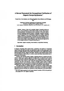
000 111 lizing GCPR, we describe a method to robustify programs. 000 111 000 111 The example highlights how our approach can be used to a) rigorously address interesting control problems for multirobot systems. 1 2 3 4 In Sec. 2, we describe GCPR for programming distributed stochastically interacting multi-robot systems and 000 111 000 111 show how GCPR can be used to address the idea of ro000 111 bustness and other control problems. In Sec. 3, we focus b) on robustness and describe a way to create robust programs by carefully adding stochastic choices in appropri1 2 3 4 ate places. Finally, in Sec. 4 we demonstrate our apFigure 1: Example multi-robot system. Four identical proach on a particular robotic platform [10], the Stochasrobotic modules that can each independently hold a brick tic Factory Floor testbed. shown at two different times. a) State in which robotic module 1 holds a brick. b) State in which robotic module 2 holds a brick.
2 Guarded Command Programming with Rates
interrupted by other commands. In contrast, commands in physical systems are never truly atomic as they take GCPR is a formal way to specify the local reactive be- time to execute. However, by appropriately designing havior of robots. Deferring a detailed description until low-level controllers to arbitrate conflicts this assumption Section 2.1, the idea is as follows. Guards are conditions is reasonable for abstract representations. on the environment of a robot. When these conditions Another benefit of GCPR that this specification is simarise, a robot can execute commands called actions that ilar to models used in formal verification. For example, modify its local environment at a specified rate. Because the modeling language of the model checker PRISM multiple guards can be true on multiple robots, multiple can be thought of as a GCP [23]. For mission critical commands can be executed simultaneously. In concur- programs such a formal description is important because rency, this situation is modeled by allowing commands to proofs about the reliability and/or correctness of such probe executed one at a time, but with arbitrary ordering [15]. grams is highly desirable. Typically, translating operaWe are obliged to reason about every possible ordering of tional code into a formal language that can be verified such executions. is tricky because what is verified is an abstract model of In the GCPR programing framework, an individual pro- the operational code. Correctness proofs are not actually gram is called a Guarded Command Program (GCP). about the code itself. While not simplifying the verifiEach robot is represented by a GCP. Multiple programs cation of the low-level code that implements sensing and running in parallel can result in interesting and complex actions, using a high-level GCP for specifying behavior behavior due to the way they interact, representing the in- paves the way for eliminating this translation step [1, 20]. teresting interactions of multi-robot systems. New GCPs that use existing guards and actions can be From the programmer perspective GCPR can also pro- verified without redoing the abstraction. vide a layer of abstraction between low-level controllers and high-level behavioral programming. By carefully 2.1 Notation choosing the level of detail of the guards and commands, GCPR can be a high-level programming language. Low- A multi-robot system evolves on a state space S, that inlevel embedded code only needs to implement the guards cludes all the relevant information. For example, the poand commands, such as recognizing and rewriting small sitions, orientations, and internal variables of all robots parts of a graph in [14]. In the GCPR framework, com- would be in S. We are interested in programming the dymands are atomic ; they are instantaneous and cannot be namics of a multi-robot system so that when the system 3
Module 1 can transition between its two occupancy states without affecting the other modules. The physical restrictions of the system are given by
starts from a set of possible initial states, it ends in a specific set of final states, the target. Using sets in this specification allows a programmer to incorporate uncertainty. Any physical system has limitations about which states are immediately accessible from a given state. For example, robots with limited speed cannot reach distant locations in short time, and robots cannot occupy the same point in space. We model such restrictions by specifying the set of possible transitions A ⊂ S × S, where the first coordinate indicates the state before a transition and the second the state after a transition.
A = Apass ∪ Aload ∪ Aunload . A graphical representation of A is shown in Fig. 2a. Each arrow corresponds to an element (s, s′ ) ∈ A, starting from s and pointing to s′ .
2.2 Syntax of Guarded Command Programming with Rates
Example 1. The first step to modeling the robotic system depicted in Fig. 1 is to decide the level of detail states should contain. To keep things simple and to illustrate the abstraction GCPR can provide, let S be the occupancy state of the system. The state will indicate which robotic modules are holding bricks. In this model each module can only be in one of two states: It can be empty (denoted by 0) or it can hold a brick (denoted by 1). As a result, states s ∈ S can be expressed as binary numbers. The state in Fig. 1a corresponds to 1000. Given a state s ∈ S, si = 1 means that the ith digit of s is 1, corresponding to a state where the ith robot module is holding a brick. Due to geometric constraints, robots can only pass bricks to their immediate neighbors. These restrictions can be captured by Apass
A GCP Ψ is a set of rules {ψi }. Each rule ψ is a triple (g, a, r) where g ⊂ S is called the guard of ψ, a predicate (true/false condition) on the state space, a ⊂ A is called the action of ψ, and r ∈ R+ (including 0) is called the rate of ψ. For each rule, when g is true, then a is applied at a rate of r, in a way that is made precise in Sec. 2.2. Example 2. A program Ψ = {(g, a, r)} for the example system from Fig. 1 that specifies passing bricks to the right is given by g ≡ a ≡ r
= {(s, s ) ∈ S × S | si = 1, sj = 0, s′i = 0, s′j = 1,
(5) (6)
Figure 2b shows a graphical representation of Ψ. Using set-builder notation is cumbersome even for such a small example and does not highlight that the reactive behavior of the robotic modules is local. To highlight this fact, we borrow notation from chemistry and write rules as chemical reactions [6]. Reactants represent the guards, they need to be present for a reaction to occur. In the chemical reaction notation, the action is to replace states in the guard with the product. The rate associated with a guarded command is written over the reaction arrow. Parts of the state that do not show up in the product remain unchanged. This notation is both more compact and emphasizes the local nature of guarded commands.
Each element of Apass represents module i passing a brick to an adjacent module j. Because the action is local, none of the other modules (k 6= i, k 6= j) change. Although not illustrated in Fig. 1, we also allow robotic module 1 to exchange bricks with an external feeding mechanism. The loading and unloading restrictions can be written as = {(s, s′ ) ∈ S × S | s1 = 0, s′1 = 1, sk = s′k , k 6= 1}
(2)
and Aunload
sj = s′j , j 6= i, j 6= i + 1} ≡ k.
′
|i − j| = 1, sk = s′k , k 6= i, k 6= j}. (1)
Aload
{s | si = 1, si+1 = 0} (4) ′ ′ ′ {(s, s ) | si = 1, si+1 = 0, si = 0, si+1 = 1,
Example 3. Using chemical reaction notation the program Ψ from Ex. 2 can be written as
= {(s, s′ ) ∈ S × S |
k
s1 = 1, s′1 = 0, sk = s′k , k 6= 1}. (3)
si si+1 ⇀ si si+1 , 4
0000
0000
0000 k
0001
1000
1000
0100
0010
1100
1010
1001
0110
0101
0011
1101
1011
0111
1110
1111
b)
k
0100 k
1100
1000
k
0100
ak k
1001
1010
k
0110
ak k
0101
ak
k
0010
k
1101
0011
0110 k
k
1011
0111
1111
1110
c)
0001
1001
ak k ak k
k
ak
k
0101 ak
k
ak
k
1100 ak
k
a)
0001
k
1010 k
1110
k
k
0010
k
1101
k
1011 ak
0011 ak
ak
0111
1111
Figure 2: Transition system from Fig. 1. a) Transitions represented by arrows show the physical limitations of the system given by A. Any program can only induce a subset of these transitions, since they represent the physical limitations of the system. b) Rates give rise to a Markov process description, programmed with Ψ. c) Markov process when the reverse is added, Ψ ∪ aΨR . where si = 1 is simply written as si while si = 0 is writ- The actions in aR correspond to physical transitions ten as si , similar to boolean algebra, note the significant whenever aR ⊆ A. simplification compared to (4)–(6) in Ex. 2. Example 4. A program for the system in Fig. 1 that For the remainder of the paper we use chemical reac- passes bricks both left and right, but passes left at a slower tion notation whenever possible. With the basic notation rate can be written as in place , the reset of this section is dedicated to defining Ψ ∪ aΨR , operations on GCP. with a ∈ (0, 1). A graphical representation of this new program is shown in Fig. 2c.
Definition 1. Composition allows two programs to operate at the same time. The composition of two GCPs Ψ and Φ is defined as Ψ ∪ Φ, (7)
A program Ψ can have several different representations. It could consist of many rules that each contain a singleton from A as actions or contain a single rule that has a large guard g and action set a. In order to compare two programs, define the function atomize that maps GCPs to GCPs on the same state space S.
the union of the two programs. Definition 2. Scaling speeds up or slows down programs. Given a program Ψ and a positive scaler ρ [ ρΨ ≡ { (g, a, ρr) }, (8)
Definition 4. The function atomize maps GCPs to representations where each rule only contains a singleton action and a trivial guard, � atomize(Ψ) ≡ ({s}, {(s, s′ )}, r) | (11) ′ (g, a, r) ∈ Ψ, s ∈ g, (s, s ) ∈ a .
(g,a,r) ∈Ψ
each rate in a program is scaled by the same number ρ. Definition 3. The reverse of a program Ψ, denoted ΨR , is the program that includes all the backward transitions of the transitions from Ψ. For a given rule (g, a, r) define gR
≡
{s | ∃s′ s.t. s′ ∈ g ∧ (s′ , s) ∈ a}
aR
≡
{(s, s′ ) | ∃s′ s.t. s′ ∈ g ∧ (s′ , s) ∈ a}. (10)
Two programs are said to be equivalent if atomize maps them to the same program. That is, they induce the same transitions with the same rates.
(9)
5
2.3
Semantics of Guarded Command Pro- work with, and as a result there are many tools for simulating and analyzing them [11, 12, 26, 30]. Section 4 shows gramming with Rates how some of these tools apply to an example multi-robot system.
The semantic meaning of a GCP is that of a Markov process. This section gives a brief definition of Markov process in Sec. 2.3.1 and collects some of the relevant results and notation in Sec. 2.3.2. Readers familiar with the subject matter can safely skim these sections for notation or skip ahead to Sec. 2.3.3 where the connection between GCP and Markov processes is made. 2.3.1
2.3.2
Properties of Markov Processes
This section collects some of the key results about finitestate Markov processes. For a more complete treatment , see for example, [30]. The hitting time for some set h ⊆ S is defined as
Markov Processes
ζh ≡ inf{t | Xt ∈ h},
Consider a finite-state, continuous-time Markov process Xt with state space S. To aid the exposition, assume some arbitrary but fixed enumeration of S, and let i ∈ S denote the ith element of S. Given two states i, j ∈ S, the transition rate from i to j is denoted by ki,j ∈ R+ . When there is no transition between states, the transition rate between them is defined as zero. Thus all pairs have an associated transition rate. Finally, one can conveniently write a differential equation for the evolution of probability distributions. Denote probability distributions on S by a vector p(t) with pi (t) ≡ P (Xt = i), and let Q be the matrix given by
and the return time as σh ≡ inf{t ≥ ζhC |Xt ∈ h},
where hC denotes the complement of h. When the process starts outside of h, ζh and σh are the same, but if X0 ∈ h , then ζh = 0 and σh is the first time that the process returns to h after leaving it. A state i ∈ S is called recurrent if P (σ{i} < ∞|X0 = i) = 1 and transient otherwise. These probabilistic quantities are closely related to the structure of possible transitions. Considering a Markov • Qji = ki,j for i 6= j process as a graph G(Q) with directed, labeled edges P highlights this connection. Define G(Q) as the triple • Qii = − j6=i Qji . G(Q) ≡ (V, E, L) where the vertex set V = S is the state space of X, the edge set E is given by E = {(i, j) ∈ The master equation [12] S × S | ki,j > 0}, and the labeling function for edges p˙ = Qp (12) L : E → R+ is given by L(i, j) = ki,j . A state j ∈ S is said to be reachable from state i ∈ S if describes the dynamics of a Markov process. By con- there exists a path from i to j in G(Q). Two states i, j are struction, the columns of the Q-matrix in (12) sum to said to communicate, written as i ↔ j, when i is reachzero, which has the following important implications for able from j and j is reachable from i. The relation ↔ is an the dynamics of a the probability vector p. Firstly, any equivalence relation that partitions S into a set of equivrow of a Q-matrix can be computed from all the other alence classes. If an equivalence class h has the property rows resulting in an at least one dimensional nullspace. that there are no states outside h that are reachable from Secondly, by left multiplying withPwith a vector of ones states in h, then all states in h are recurrent. P it should be clear that i p(t) = i p(0), which should be identically equal to 1 in order to represent probability Example 5. Figures 2b and 2c are graphical represendistributions over states. In general, by analyzing proper- tations of Markov processes. In Fig. 2b, each state is ties of this matrix one can infer properties of the stochas- an equivalence class. Figure 2c has equivalence classes tic process, for example, the steady-state distribution(s), {0000}, {1000, 0100, 0010, 0001}, {1100, 1010, 1001, the convergence rate, or the hitting times (Sec. 2.3.2). 0110, 0101, 0011}, {1110, 1101, 1011, 0111}, and Markov processes are convenient stochastic processes to {1111}, all of which are recurrent. 6
0000 bk
graphs and its consequences for Markov processes. For a more thorough treatment, see, for example, [5, III.2]. A graph G is said to be connected if any two vertices have a path between them. A connected graph G is said to be separated by a set of vertices h ⊂ V if the graph induced by removing h is no longer connected. A graph is said to be k-connected when there is no set of k − 1 vertices that separates it. The largest value of k for which a graph G is k-connected is called the connectivity, denoted κ(G). For two sets h, h′ ⊂ V , we define the restricted connectivity κ(h, h′ ) to be the largest k such that no set of k − 1 vertices removed from h disconnects vertices in h from h′ (i.e., there is a path from every s ∈ h to some vertex in h′ ). When comparing the connectivity for graphs induced by different Q-matrices, a subscript to κ denotes the corresponding Q-matrix.
bk k
1000
k
0100
ak bk bk k
1100
ak bk
bk
1010
1110
bk
ak
bk
0001 bk
1001
k
ak ak k
0110 bk k
ak
k
ak ak
k
0010
k k
0101 ak bk bk k
1101
0011 ak
bk
bk k
1011 ak
0111
ak bk
bk
1111
Figure 3: Transition system from Fig. 2c with loading program added. The resulting Markov process has a single recurrent equivalence class.
Example 6. In Fig. 2b and 2c the graph associated with the Markov process is not connected. The connectivity κ for the graph in Fig. 3 is one (for example, 1000 separates the graph), while the restricted connectivity κ(h, h′ ) where
To create a program with a single recurrence class, a loading and unloading program Φ needs to be added to Ex. 4, otherwise the conservation of bricks restricts the communicating states to contain states with the same number of bricks. Let Φ be k
s0 ⇀ s0
h = {0100, 0010, 0001, 1100, 1010, 1001}
k
s0 ⇀ s0 .
h′ = {0110, 0101, 0011},
The program given by Ψ ∪ aΨR ∪ bΦ
is 2.
has a single recurrence class because all states communicate (Fig 3).
2.3.3
For a finite-state process the Q-matrix is always singular and has non-positive eigenvalues. Hence, for any initial distribution p(0), the limit
To define a Markov process on S it suffices to specify a Q-matrix and an initial probability distribution on S. To construct Q(Ψ), define the set of rules
πQ ≡ lim p(t)
Turning Guarded Command Programs Into Markov Processes
Ri,j = {(g, a, r) ∈ Ψ | i ∈ g, (i, j) ∈ a}
t→∞
exists. When there is only a single recurrent communicating class, this limit is unique , and πQ is called the steady-state distribution. Only recurrent states have positive probability in πQ . The largest negative eigenvalue λ2 (Q) is the worst-case convergence rate to πQ from any initial condition. In addition to the standard observations connecting discrete-state Markov processes with their graphs, the remainder of this section examines the connectivity of
(13)
that make transitions from state i ∈ S to state j ∈ S. The entries of Q(Ψ) are given by P • Q(Ψ)ji = ψ∈Ri,j rψ for i 6= j • Q(Ψ)ii = −
P
j6=i
Q(Ψ)ji ,
where rψ is the rate of rule ψ. The dynamics of the system with program Ψ are given by the master equation (12). 7
Example 7. Take the GCP described in Ex. 2 and Ex. 3, with the enumeration of states in Fig. 2 from the upper left to lower right (i.e., the enumeration 0000, 1000, 0100, 0010, 0001, 1100, 1010, 1001, 0110, 0101, 0011, 1110, 1101, 1011, 0111, 1111) the associated Q-matrix is the 16-by-16 matrix 0 0 0 0 0 0 Q1 0 0 0 Q(Ψ) = 0 0 Q2 0 0 0 0 0 Q1 0 0 0 0 0 0 with
and
−k k Q1 = 0 0
Q2 =
−k k 0 0 0 0
0 −2k k k 0 0
programs ). The inherent randomness of each program makes the composition of two programs easy; how actions interleave is random. Although detailed timing information is difficult to express in this framework, it is easy to adjust the relative influence of concurrent programs by scaling them up or down. Together scaling and compositions, are sufficient for expressing a number of interesting control problems, Sec. 2.5. Additionally, we gain the ability to incorporate statistical failure information and uncertainty, as pointed out in Sec. 1.
2.4 Operations on Q-matrices
0 −k k 0
0 0 −k k
0 0 0 0
0 0 −k 0 k 0
0 0 0 −k k 0
0 0 0 0 −k k
Composition, scaling, reverse, and atomize operations on GCPs (Def. 1–4) correspond directly to operations on their associated Q-matrices.
0 0 0 0 0 0
Linear Composition 1. Given any two GCPs Ψ and Φ on the same state space, and two positive scalers γ1 , γ2 ∈ R+ , the following equation holds
,
Q(γ1 Ψ ∪ γ2 Φ) = γ1 Q(Ψ) + γ2 Q(Φ).
(14)
′ Ri,j
Proof. Define Ri,j for Ψ and for Φ as in (13). For the off-diagonal elements i 6= j we have γ1 Q(Ψ)ji + γ2 Q(Φ)ji X X ′ = γ2 rψ γ1 rψ +
where 0 denotes a matrix of zeros of compatible dimen′ ψ∈Ri,j ψ∈Ri,j sion. The block diagonal structure of Q(Ψ) corresponds to the fact that the number of bricks in the system is con= Q(γ1 Ψ ∪ γ2 Φ). served. Each block corresponds to a different number of bricks. The 0 entries at the top and bottom correspond to Because the diagonal elements are computed from the the state when there are no bricks and when all modules off-diagonal entries in each column, (14) follows. are holding bricks respectively. In either case, no transiThe Q-matrix of the reverse of a program is the same tions are possible with Ψ, which does not have loading or as the transpose of the generator for the forward program unloading rules. except that the diagonal is different. To highlight this conIn a GCP , a programmer can only specify the aver- nection, define the matrix A with entries � P age rate at which actions are applied conditioned on the i 6= j ψ∈Ri,j rψ A(Ψ) = guard. Typically, the rate the inverse of the mean compleji 0 otherwise. tion time of the assoicated action. The Markov process semantics mean robots randomly choose when to execute The A-matrix is the same as the Q-matrix except that it commands if their guards are true. This loose timing con- has zero entries on the diagonal. However, the diagonal straint is in stark contrast to other ways of programming can be computed from the other entries. In particular, multi-robot systems where the timing of actions is careQ(Ψ) = A(Ψ) − diag(AT (Ψ)1), fully specified. These semantics are a compromise between the ability to specify timing and the ease of operat- where 1 denotes a vector of ones with compatible dimening on programs (i.e., the ease of composing and scaling sion, and T denotes the transpose of a matrix. 8
reusable code. For example, if Ψ is a program that disassembles a structure and Φ transports raw materials, then
Lemma 2. The reverse of a GCP Ψ is given by Q(ΨR ) = AT (Ψ) − diag(A(Ψ)1).
Ψ∪Φ Proof. By construction, Q(ΨR )ij = A(ΨR )ij for i 6= j. By the same argument as in the proof in Lem. 1, it suffices to consider off-diagonal elements and show that A(ΨR ) is equal to A(Ψ)T . Looking at these two matrices element wise yields X A(ΨR )ji = rψ =
X
is a program that does both (Ex. 4). In general, composing arbitrary concurrent programs, while well defined, does not yield desirable new programs. A programmer needs to be aware of how the actions of two GCP interact. One way of ensuring sensible compositions is to construct programs where the sink state of one is the input for another. Control Input: In a system that has both natural dynamics Ψ and some other dynamics Φ that we have direct control over , the composition
ψ∈Ri,j (ΨR )
rψ = A(Ψ)ij
ψ∈Rj,i (Ψ)
= A(Ψ)Tji .
Ψ ∪ uΦ,
where u ∈ R+ describes a system with a control input. Lemma 3. A program and its atomized version have the For example, open-loop optimal control in Sec. 4.2.5 or [18] and feedback control [27] can be implemented by same Q-matrix using a system description of this form. In the context of multi-robot construction systems, the control input is parQ(Ψ) = Q(atomize(Ψ)). ticularly useful for balancing programs that correspond Proof. This lemma follows directly from the definition of to different subtasks, such as disassembly, routing, and atomize, which keeps all elements of each action a from building sub-programs. the original program, but creates a new rule for each one. Disturbances: Similarly, consider a nominal system Ψ and a set of undesirable transitions denoted by Φ. The composition The mapping of programs to Q-matrices allows us Ψ ∪ εΦ, to reason about new, composed programs by examining where ε ∈ R+ describes uncertainty around a nominal properties of the corresponding matrices. model Ψ. The program Φ can either contain disturbances or previously unmodeled transitions. In the latter case, 2.5 Control Problems Expressed with when S contains failure states, Φ can be used to express Guarded Command Programs failure statistics (Sec. 4.3). Inaccessible States: Different failure scenarios where apThe ability to scale and compose programs allows us to plied actions might not cause transitions due to intermitframe questions about programming and control of multitent malfunctions or states become inaccessible due to robot systems with GCPs. In the following discussion broken subsystems can also be modeled with GCPs. A programs are assumed to have similar rates, so a program given GCP Ψ can be decomposed into an equivalent promultiplied by a small scaler has lower rates than a program gram that is not scaled. This assumption corresponds to ΨW ∪ ΨB , the fact that physical robots can only execute actions at a fixed maximal rate and that programs that express behav- where ΨB corresponds to the part of the program that is iors execute these behaviors as quickly as possible. malfunctioning and ΨW the part of the program that is Modularity: By composing subprograms which can working correctly (Sec. 3.2.1). Intermittent failures can be separately written and analyzed allows us to create be expressed as ΨW ∪ (1 − λ)ΨB , where λ ∈ (0, 1) is 9
3.2 Types of Disturbances
the strength of the intermittent fault. Larger values of λ correspond to a larger likelihood the faulty behavior. Permanent failures of subsystem can be modeled by only considering working transition ΨW .
3.2.1
Program Decomposition
As described in Sec. 2.5 , modeling inaccessible states can be accomplished by decomposing a program Ψ into two parts. Given a set of states that are broken SB ⊂ S, the set of states that are still accessible or working is SW = S \ SB . Given a program Ψ and a set of broken states , we describe how to construct an equivalent program ΨW ∪ ΨB where the program ΨW only makes transitions between states in SW .
3 Robustifying Programs
This section presents an approach to combine a high performance and a robust GCP to obtain a new program with the best qualities of both. We refer to this process as “ro- Definition 5. Each rule in ψ ∈ Ψ is either in ΨW , ΨB , or bustification” because it can turn a program that is not split into two parts as follows. Given a ψ = (g, a, r) ∈ Ψ robust into one that is, while preserving qualities of the define the a rule ψB ≡ (gB , aB , rB ) by original program [28]. rB ≡ r (15) A robust program is one that behaves correctly in the a ≡ a ∩ (S × S ∪ S × S) (16) face of disturbances. Both correctness and the class of B B B disturbances need to be defined. We consider a program gB ≡ (g ∩ SB ) ∪ {s | (s, s′ ) ∈ aB }. (17) to be correct when it has probability one of ending up in a pre-specified region in the state space called the target, The working part of the rule is the complement ψW = T . In the language of stochastic processes, only processes (gW , aW , rW ) = (g \ gB , a \ aB , r). Whether a rule where the recurrent states are contained in the target have ψ ∈ Ψ belongs to ΨB , ΨW , or is split according to (15)– correct behavior. This definition of is motivated by our (17) is decided as follows: constructive approach to writing modular programs. By • If aB = ∅, then the ψ ∈ ΨW . choosing the target of one program as the input to the next several programs can be strung together. A description of • If aW = ∅, then ψ ∈ ΨB . the disturbances is given in Sec. 3.2.
• If aB 6= ∅∧aW 6= ∅, then ψB ∈ ΨB and ψW ∈ ΨW .
3.1
A program can be split into two parts by applying the above procedure to all its rules.
Program Performance
The performance of a program is the rate at which arbitrary initial probability distributions converge to the steady-state distribution. If distributions converge quickly, a program is said to have good performance . If distributions take a long time to converge , it has poor performance. Numerically, the performance of a program Ψ is bound by the second largest eigenvalue of Q(Ψ), denoted λ2 (Q). It is a measure of convergence rate in the master equation (12). The greater the magnitude (more negative) the second eigenvalue the faster the convergence rate. Multiple zero eigenvalues, correspond to the case of multiple recurrent equivalence classes. 10
Theorem 4. Given a GCP Ψ and set SB , the construction in Def. 5 results in two programs ΨB and ΨW with the property that ΨB ∪ ΨW is equivalent to Ψ. Proof. By construction, the elements of a for each ψ ∈ Ψ appear in a rule of either ΨB or ΨW with the original rate. As a result atomize(Ψ) = atomize(ΨW ∪ ΨB ), and so the decomposition produces an equivalent program.
3.2.2
Intermittent Failures
There are two different types of intermittent failures. Firstly, imagine there are some transitions in a given GCP Ψ that depend on faulty hardware. Maybe the gripper of a robot has a loose screw and occasionally drops an object. A low-level controller recovers from the error and puts the system back into the state before the transitions. In general, sometimes when a command corresponding to a faulty transition executes, it does not work. Instead, the system remains in the original state. As described in the discussion of inaccessible states in Sec. 2.5, a program with intermittent faults of this type can be written as
3.3 The Performance and Robustness of Composed Programs This section gives two theorems about the composition of programs. Both are about the continuity of composition. Adding a small amount of an arbitrary program Φ to a nominal program Ψ means that the composition will have a similar steady state and convergence rate as Ψ. The theorems are stated in terms of the Q-matrices associated with GCPs. Lemma 5. Given two Q-matrices A and B with the same dimension, then ∀δ > 0, ∃ε > 0 such that
ΨW ∪ (1 − ρ)ΨB ,
|λ2 (A) − λ2 (A + εB)| < δ.
where ρ ∈ (0, 1) is the intensity. Secondly, instead of returning to the original state after an intermittent fault the system could end up in a state that is neither the first nor the second coordinate of the action. For example, a gripper could occasionally drop an object that is not recovered by a low lever controller. This type of intermittent failure can be expressed as a disturbance (Sec. 2.5) Ψ ∪ εΦ,
Proof. The eigenvalues of A + εB are the solutions of the characteristic polynomial, det (λI − (A + εB)) = 0. The roots of a polynomial are continuous functions of the coefficients, which in turn are continuous functions of ε. By composition on continuous function the eigenvalues of A + εB depend continuously on ε. Lemma 6. Given Q-matrices A and B of two correct programs with the same target h ⊂ S, then for C = A + B,
where the disturbance program Φ contains intermittent and unintended transitions occurring with intensity ε. 3.2.3
κC (hC , h) ≥ max{κA (hC , h), κB (hC , h)}.
Permanently Inaccessible States
Modeling a specific permanent failure where states become inaccessible is simpler. Given a program Ψ and a set of broken states SB , by Thm. 4, Ψcan be decomposed into an equivalent program ΨW ∪ ΨB . The working part ΨW only makes transitions in SW . Using it as a new program on SW models the behavior of the system where some of the states have become permanently inaccessible. The permanent failure case is the limit of the recoverable failure case when λ → 1. By construction all the states in SB are recurrent and do not communicate, when considering only the working program ΨW , because all transitions to and from states in SB have been removed from ΨW . One must take care in any subsequent analysis to considering questions about the connectivity of ΨW only on SW . 11
Proof. Adding two Q-matrices can only increase the number of (vertex) independent paths from hC to h; therefore, κC (hC , h) is at least as large as κA (hC , h) and κB (hC , h). Theorem 7. Given a Q-matrix A with a single recurrent communicating class and some other Q-matrix B, then C = A + εB where 0 ≤ ε has a single recurrence class , and the entries of πC depend continuously on ε. Proof. By assumption about A, C also has a single recurrence class and thus a unique steady-state distribution πc . Furthermore, πc is the intersection of the one dimensional subspace given by the flux balance equation Cp = 0 and the hyper plane given by the probability vector constraint 1T p = 1. Since these are linear constraints with coefficients that vary continuously on ε, the entries of πC also depend continuously on ε.
Hence, varying ε cannot produce a bifurcation in equilibrium points when adding εB to the Q-matrix A . However, in general when A does not have a single recurrence class (dim(null(A)) > 1) adding εB to A can make steady-state solutions disappear. In particular, a transition in B may connect two different recurrent equivalence classes, and the steady state from a given initial condition might not be continuous in ε. Including the condition on the number of recurrent classes in Thm. 7 is necessary. Theorem 8. Given two Q-matrices A and B with the same, unique recurrent state s∗ , then for any δ > 0, ∃ ε > 0 such that for C = A + εB,
b)
• |λ2 (A) − λ2 (C)| < δ • κC ({s∗ }C , {s∗ }) ≥ κB ({s∗ }C , {s∗ }) • π C = πA .
c)
a)
Theorem 8 follows directly from applying Lemmas 5 and 6. Both Thm. 7 and 8 are about composing a nominal program Ψ (represented by A) with other programs. By Lem. 5 , if Ψ is composed with some sufficiently small amount of an arbitrary program Φ , then the the convergence rate of Ψ+εΦ is close to the convergence rate of Ψ. By Thm. 7 , the steady-state distribution of Ψ and Ψ + εΦ are also close element wise. Thm. 8 is about composing programs that are both correct (with respect to the same target state s∗ ) but can have different performance and robustness. It states that one can add a robust (high relative connectivity) program with a high performance program (|λ2 | large) and obtain a program that has both good performance and robustness.
4 The Factory Floor Testbed This section describes an extended example demonstrating how to apply Thm. 8 to the Factory Floor testbed, a multi-robot system that can assemble, disassemble, and reconfigure structures [10]. The goal of this testbed is to aid development of robust algorithms and hardware that can autonomously build structures in uncertain environments. 12
d)
e)
Figure 4: The Factory Floor testbed [10]. a) Schematic representation of a Factory Floor module. b) Picture of truss type raw material. c) Picture of node type raw material. d) Picture of four modules assembling a two layer structure. e) Picture of same structure in simulation. For clarity, module components are omitted, and only the raw materials are shown.
4.1 Description
a)
b)
c)
d)
The testbed [10] consists of an array of identical robotic modules that build structures made from two different types of raw material called trusses and nodes (Fig. 4). Each module has a manipulator with an end effector that can grab and release nodes and trusses, a temporary storage place for nodes and trusses, and a lifting mechanism. Assembly and disassembly proceed layer by layer. Modules manipulate raw materials into place and then coordinate lifting with other modules. At the end of each truss is a latching mechanism that can be activated by the end effector and rigidly attach to one of the six node faces. By this mechanism the Factory Floor testbed can build arbitrary lattice structures from trusses and nodes. The sequence of pictures in Fig. 5 shows a typical reconfiguration task. A tower is disassembled on one side of the testbed, the raw materials are routed, and then a tower is assembled on the opposite side. Figure 5f shows which modules in the testbed run the three different tasks.
4.2 Routing Programs
This section describes programs for the routing portion of the reconfiguration task in Fig. 5 in more detail. This subtask is performed by the most modules and as a result has the most redundancy, which is important to the robustness to module failure. Programs can only be robust to individual robot failures if there are redundant robots. Fig. 6a gives the layout of the factory floor testbed for the configuration task. The hashed modules {1, 2, 3, 4} e) f) and shaded modules {18, 19, 22, 23} correspond to the Figure 5: Sequence of snap shots from a reconfigura- loading area (L) and the target area (T ), respectively. tion simulation. The sequence a-e) shows the program Each module either has a node or not, and so the state at various stages of progress a) Initial configuration. e) of each module is binary, which is similar to Ex. 1. The Final goal configuration. f) Image sowing loading area L state of a module is 1 when the module contains a node (hashed), routing area R (white, right), and the target area and 0 when it does not. In the routing portion of a reconT (shaded) of the routing program (Fig. 6). To the left figuration program, what happens in the target area is not of L a GCP running in the disassembly area (white, left) important. During routing, it acts as a sink, and nodes takes a structure apart and feeds the raw materials to the disappear as soon as they get into the target area. As a result, the four modules in T can be lumped together routing program. resulting in the state space S = {1, 0}21 , that is, the 21fold cross product of the module state, a 21 digit binary number as in Ex. 1. Figure 6b and Fig. 6c show two different routing programs. Each arrow represents a rule of a GCP, and 13
11 00 00 11 00 11 00 11 00 11 00 11 00 11 00 11 b) 11 00
111 000 000 111 000 111 000 111 000 111 000 111 000 111 000 111 a) 000 111 1
5
9
2
6
10 14 18 22
3
7
11 15 19 23
4
8
12 16 20 24
13 17 21
a)
111 000 000 111 000 111 000 111 000 111 000 111 000 111 000 111 000 111 c) 000 111
b)
c)
Figure 7: Three different failure scenarios. a) All modules are working. b) Module 10 is broken, c) Module 10 and 11 are both broken. 4.2.1
Performance Without Failures
To analyze the performance and robustness of these sysFigure 6: Schematic representations of routing programs. tems we look at how a program routes a single node. This The loading area L is denoted by hashed modules, the assumption drastically reduces the size of the state space , routing area R by white modules, and the target area T yet the connectivity properties governing the robustness in by shaded modules. a) Layout of the factory floor testbed. the single-node case carry over to the general case withThe numbers in each module position identify the module out this restriction. When only allowing one node at a when writing programs. b) Deterministic path program time, the state space of the system is simply the position Ψ. Only transitions that provide progress are enabled. c) of that node. When a module fails and stops routing nodes Random Program Φ. In each location all possible transi- , only a single state (but multiple transitions) become untions are enabled. This program is slow since many of the available. In this simplified problem , a node randomly appears transitions do not provide progress toward the target area. in the loading area either from an external source or, as in this example, from a disassembly program. The uneach module runs a program containing all the rules cor- certainty in the loading is expressed as a probability disresponding to arrows in that location. Using chemical re- tribution of where the node shows up. The target area is action notation as in Ex. 3 programs for the Factory Floor modeled as a single state that only accepts nodes. When all modules operate correctly , it is easy to see that nodes modules can be written as will be routed to the single accepting sink state (T ). With kpass kpass = kload = 1sec−1 , the rate of convergence (|λ2 |) s3 , s7 ⇀ s3 , s7 of the two programs Ψ and Φ shown in Fig. 6 is 1.0 and kload s3 s3 ⇀ 0.029 , respectively. Both programs are correct, but Ψ has much better performance. in the case of module 3 in Fig. 6b, for example. The associated rates are such that the rates of all rules 4.2.2 Modeling Specific Failures corresponding to actions performed by the same module sum to a constant kpass . This rate models the speed at The first step is to consider failures of specific modules. which modules perform tasks, in this case how long it Similar to considering only a single node at a time , this takes to pass raw materials. The average time to pass raw approach yields small, tractable Markov processes and almaterials is 1/kpass . If there are multiple arrows, then each lows us to gain some intuition before tackling a more genof the associated guarded commands has the same frac- eral model that incorporates failure statistics. The three tion of the total rate kpass . Also, nodes appear randomly specific scenarios we considered in this section , which in the loading area L at a rate kload . In this way , the are shown in Figs. 7a–c, are the cases when there are: no diagram Figs. 6b and 6c can be turned into guarded com- failures, a single-module failure, and multiple-module mand programs with rates. We denote the program from failure. We apply Thm. 4 to the two failure scenarios. In the Figs. 6b and 6c by Ψ and Φ , respectively. 14
case of a single failure (module 10 in Fig. 7b), the set of broken states is SB = {s ∈ S|s10 = 1}. Applying Thm. 4 to Ψ (Fig. 6b) results in ΨB , kpass
s6 s10 ⇀ s6 s10
kpass
s10 s14 ⇀ s10 s14 . Intermittent faults in Module 10
This decomposition is simple because the rules in Ψ are written in chemical reaction notation to begin with and each rule belongs either to ΨB or ΨW . The other rules of Ψ are in ΨW . The chemical reaction notation is also applicable to the broken part of Φ (Fig. 6c). The broken component ΦB is kpass
s6 s10 ⇀ s6 s10 kpass
s14 s10 ⇀ s14 s10 kpass
s9 s10 ⇀ s9 s10 kpass
s11 s10 ⇀ s11 s10
Ψ Φ Θ
1
2
Performace |λ |
0.8
kpass
0.6
0.4
0.2
s10 s6 ⇀ s10 s6 kpass
0
s10 s14 ⇀ s10 s14
0
0.1
0.2
0.3
0.4
a)
kpass
s10 s9 ⇀ s10 s9
0.5
ρ
0.6
0.7
0.8
0.9
Intermittent faults in Module 10 and 11
kpass
Ψ Φ Θ
1
s10 s11 ⇀ s10 s11 .
0.8
2
Performace |λ |
The broken components ΨB and ΦB for the failure of multiple modules (Fig. 7c) work exactly the same except that they contain more reactions. Using these compositions , one can model both intermittent and permanent failures.
0.6
0.4
0.2
0
4.2.3
Performance with Intermittent Faults
b)
By combining the two parts of a decomposed program (e.g. ΨW and ΨB ), one can investigate the performance of Ψ with intermittent failures. The probability of an intermittent failure is given by ρ ∈ (0, 1). Because we restrict the failure probability to be less than 1, all states that communicate in Ψ also communicate in ΨW ∪(1−ρ)ΨB . As a result, programs with intermittent faults have the same equivalence classes with the same recurrence structure. If the original program Ψ is correct, then the program with intermittent faults is also correct. However, the performance can degrade significantly. Figure 8 shows the second largest eigenvalue λ2 of ΨW ∪ (1 − ρ)ΨB and ΦW ∪ (1 − ρ)ΦB as a function of ρ for the two different failure scenarios shown in Fig 7.
0
0.1
0.2
0.3
0.4
0.5
0.6
0.7
0.8
0.9
ρ
Figure 8: Performance (λ2 ) as a function of fault intensity ρ. a) Performance of Ψ (solid line), Φ (dashed line), and Θ (dash-dotted line) with a single, intermittent fault (Fig. 7b). c) Performance of Ψ, Φ, and Θ = 0.9Ψ + 0.1Φ (see Sec. 4.2.4) with two intermittent faults (Fig. 7c).
15
4.2.4
Performance with Permanent Failures
No Malfunctions
Probablity of Arrival
1
In contrast to intermittent failures, permanent failures can change the recurrence structure of a program. These types of failures can turn a correct program into one that is no longer correct.
By Thm. 8 , we can combine both programs and obtain one that is robust and has good performance. For example, choosing ε = 0.1 , the program Θ = (1 − ε)Ψ + εΦ has λ2 = −0.66 and the same robustness as Φ. This means that ΘW = ΨW ∪ ΦW should be correct and have good performance. The reason to choose a convex combinations of programs instead of other scaled compositions is to conserve the total rate of passing raw materials for each module, which is necessary for a sensible physical interpretation of the resulting program. Figure 8 compares the performance of these three programs in the case of intermittent faults, and here too, Θ has most of the desirable performance features from Ψ.
a)
0.6
0.4
0.2
0
Ψ Φ Θ 0
20
40
60
80
100
120
140
160
180
200
time
Module 10 Malfunction 1
Probablity of Arrival
Section 4.2.1 shows that Ψ has better performance in the absence of failures, but when any routing modules fail permanently , the resulting Q-matrix has multiple recurrent equivalence classes with some recurrent states outside the target. In contrast, Φ has the opposite problem, it has low performance due to the backward passes that do not provide progress, but it performs correctly when up to three modules fail because the relative connectivity to the target is κ(L ∪ R, T ) = 4.
0.8
0.8
0.6
0.4
0.2
b)
0
Ψ Φ Θ 0
20
40
60
80
100
120
140
160
180
200
time
Module 10 and 11 Malfunction
Probablity of Arrival
1
c)
Exactly how these programs fair in the failure scenarios is shown in Fig. 9. The top of each sub-figure shows which modules have failed. The plot on the bottom shows the probability of arriving as a function of time given that a node showed up in the loading area at time 0. With no failures (Fig. 9a) , the three different programs behave as described in Sec. 4.2.1 ; all programs are correct, and Ψ and Θ have good performance while Φ has bad performance. Failure scenarios where one and two modules fail are shown in Figs. 9b and 9c. With failures, only ΦW and ΘW behave correctly ; they are robust to failure. The program ΘW has good performance and is robust. This demonstrates how one can use composition to combine the desirable properties of robust programs and high-performance programs. 16
0.8
0.6
0.4
0.2
0
Ψ Φ Θ 0
20
40
60
80
100
120
140
160
180
200
time
Figure 9: Program performance with various failure scenarios. The plots show the probability of a node arriving at the target (given it was at the loading area at t = 0) as a function of time. The solid line corresponds to the program Ψ shown in Fig. 6b , the dashed line to the program Φ shown in Fig. 6c, and the dash-dotted line to the composed program Θ = 0.9Ψ + 0.1Φ. a) Programs with no module failures, Ψ and Θ have similar good performance , and Θ has poor performance. All programs are correct. b,c) Programs with one and two module failures respectively. Only Θ and Φ are correct; they are robust to module failure.
4.2.5
The robustification in the previous section shows that a convex combination of programs can yield desirable results. Exactly how programs should be weighted depends on the particular problem. In the context of the Factory Floor testbed we look at two different measures of quality. First, the time of 90% probability of arrival (Sec. 4.2.4). Figure 10a shows the time it takes for the probability of routing a node to the target with 0.9 probability of success, given that it shows up randomly uniformly distributed in the loading area at t = 0. Depending on the failure scenario, the best choice of ε is different. Second, the performance λ2 of the convex combination (Fig. 10b), results in a different optimal of ε, which again depends on the failure scenario. Since the performance depends on the scaler parameter of the convex combination, the problem of choosing it can be turned into an optimization problem. For a more detailed description of a particular problem and how to solve the resulting optimization problem, see, for example, [18]. Here, we simply want to point out that GCPR can be used to pose questions of writing high quality programs as an optimization problem using convex combinations of GCPs. While the parameter space is convex these problems are not necessarily easy to solve because the quality measure of programs can be numerically expensive to compute.
Speed vs. ε 110 100 90
t
p=0.9
80 70 60 50 40 30 1 Broken 2 Broken
20 10 0.1
0.2
0.3
0.4
0.5
a)
ε
0.6
0.7
0.8
0.9
1
Performace vs. ε 0.16 1 Broken 2 Broken
0.14 0.12 0.1
|λ2|
Optimizing Programs
0.08 0.06 0.04 0.02 0
b)
0
0.1
0.2
0.3
0.4
0.5
ε
0.6
0.7
0.8
0.9
1
4.3 Incorporating Failure Statistics
Figure 10: Quality measures of (1 − ε)Ψ ∪ εΦ. a) Time of 90% arrival as a function of ε with two different failure scenarios (Figs. 7b and 7c) . b) Performance |λ2 | as a function of two different failure scenarios (Figs. 7b and 7c).
17
The stochastic nature of GCPR can easily incorporate failure models based on empirical, statistical information. It is particularly easy to incorporate failures that are exponentially distributed. More complicated distributions can be approximated by using a series of failure states with exponential transitions between them. This section is a slight departure from the previous sections because it requires expanding the underlying state space S to capture failures. To do so in this particular example, we extend the state of each module to include a failure state, and so S = {0, 1, 2}21 instead of just including two states per module. If a module is in state 2 , it has failed and can no longer pass nodes or trusses. We can still use the old programs, Ψ, Φ, and Θ, from the previous sections embedded into this new higher di-
Program Ψ Φ 0.9Ψ ∪ 0.1Φ Ψ ∪ Γ Φ ∪ Γ 0.9Ψ ∪ 0.1Φ ∪ Γ
mensional state space. The chemical reaction notation makes this embedding easy because it only specifies the part of the state that changes, and the original states, 0 and 1, are still in the expanded state space. To express failures of modules in chemical reaction notation, denote the situation that the ith component (module i) of s ∈ S is broken by sei (i.e., sei = 2). If individual modules fail at a rate of kfail , a program Γ that models this failure can be written as
Mean (95% CI) 357.5 ±1.1 197.7 ±0.5 353.7 ±1.0 79.7 ±2.6 65.2 ±1.7 96.6 ±2.9
STD 16.7 8.3 16.3 41.0 27.2 45.7
Table 1: Mean number of routed nodes. Trajectories were simulated for 1000sec with rate parameters kfail kfail sei . si ⇀ sei si ⇀ kpass = 1sec−1 , kload = 0.1sec−1 , and kfail = 0.001sec−1 This new state space is quite large (321 ≈ 2.8 × 10¹¹ ) using SSA. The parameters are chosen such that trajec, so computing the probability distribution over states tories have the same length as the mean time to failure or the eigenvalues of the transition matrix is difficult. of modules. The mean and the standard deviation were However, simulating trajectories and estimating statisti- computed from 1,000 trajectories. cal quantities can be done efficiently using the Stochastic Simulation Algorithm (SSA) [11]. Table 1 shows SSA re- also behaves much better than Ψ when incorporating stasults to estimate the expected number of routed nodes in tistical failure. This extended example shows how GCPR the first 1000sec for Ψ, Φ, Θ, Ψ ∪ Γ, Φ ∪ Γ, and Θ ∪ Γ can be used as a flexible tool in programing and reasonwith a failure rate of kfail = 0.001sec−1 , a loading rate ing about the behavior of stochastically interacting robots. of kload = 0.1sec−1 , and a passing rate kpass = 1sec−1 . We created a manageable simplified model (single node) The simulation time is the average life-time of a mod- to design a routing program Θ via robustification. These ule 1/kfail . With this choice a significant number (50%) simulation results suggest that this GCP also performs of the modules are expected to break by the end of sim- well in the non-simplified system. ulation. Obviously, the number of routed parts is significantly higher for the programs that do not contain the failure program Γ, and Θ is almost as good as Ψ in the 5 Conclusion absence of permanent failures, and behaves significantly better when failures are present. Given the simulation Stochasticity can be used to model concurrency, failures, time and failure rate of this example, the final state of each and uncertainty. We use it to give semantic meaning to trajectory is expected to have half of its modules broken. GCPR and use the resulting framework to create robust With such a sever fraction of broken modules, it is likely programs with good performance. The main contribution that there is no routing path from the from the loading of this paper is framing the problem of multi-robot proarea to the target. The data reflects this in two ways. First, gramming formally as GCPR. The operations of compothe significantly lower mean of the programs that contain sition, scaling, reverse, and decomposition can express Γ, and second, the much higher standard deviation of the a variety of control questions related to multi-robot sysprograms with failures even though the mean is lower. tems. We show that these operations on programs are diThe increased variance results from the fact that the ef- rectly related to operations on the generators of Markov fectiveness of the routing program is randomly decreased processes, and so the analysis of composed and scaled by broken modules. This additional source of randomness programs can be drastically simplified This approach differs fundamentally from other apincreases variance. We expect this source of noise to be the least effective in the case of Φ, since purely random proaches in which robot behavior is deterministic. Alexploration should effectively explore paths around bro- though these semantics are restrictive in some sense, GCPR is sufficiently expressive to pose interesting probken modules, where as Ψ and Φ do not. The GCP Θ created in the previous section to be more lems while facilitating composition of programs, somerobust to failures in the simplified, single-node model thing that is difficult to reason about with other ways of 18
programming. We show how composition and scaling of programs can be used to express a variety of control questions and focus on robustness in an extended example of a routing program that is part of larger reconfiguration task.
[10] K. Galloway, R. Jois, and M. Yim. Factory floor: A robotically reconfigurable construction platform. In Proceedings of IEEE International Conference on Robotics and Automation, pages 2467–2472, Anchorage, AK, USA, 2010.
References
[11] D.T. Gillespie. Stochastic simulation of chemical kinetics. Annual Review of Physical Chemistry, 58(1):35–55, 2007.
[1] R. Alur, Thao Dang, J. Esposito, Yerang Hur, F. Ivancic, V. Kumar, P. Mishra, G.J. Pappas, and O. Sokolsky. Hierarchical modeling and analysis of embedded systems. Proceedings of the IEEE, 91(1):11–28, Jan. 2003.
[12] N.G. Van Kampen. Stochastic Processes in Physics and Chemistry. Elsevier, 3rd edition, 2007.
´ H´al´asz, M. Yim, and [2] N. Ayanian, P. White, A. V. Kumar. Stochastic control for self-assembly of XBots. In ASME Mechanisms and Robotics Conference, New York, August 2008.
[13] E. Klavins. Automatic compilation of concurrent hybrid factories from product assembly specifications. In Proceedings of Hybrid Systems: Computation and Control, number 1790 in LNCS, pages 174–187. Springer-Verlag, 2000.
[3] T. Balch and R. C. Arkin. Behavior-based formation control for multirobot teams. IEEE Transactions on Automatic Control, 14(6):926–939, 1998.
[14] E. Klavins. Programmable self-assembly. IEEE Control Systems Magazine, 27(4):43–56, Aug. 2007.
´ H´al´asz, and A. Hsieh. Optimized [4] S. Berman, A. stochastic policies for task allocation in swarms of robots. IEEE Transactions on Robotics, 25(4):927– 937, Aug. 2009.
[15] E. Klavins, R. Ghrist, and D. Lipsky. Graph grammars for self-assembling robotic systems. In Proceedings of IEEE International Conference on Robotics and Automation, pages 5293 – 5300, New Orleans, LA, USA, 2004.
[5] B. Bollob´as. Modern Graph Theory. Springer, 1998. [6] S. Burden, N. Napp, and E. Klavins. The statistical dynamics of programmed robotic self-assembly. In Proceedings of IEEE International Conference on Robotics and Automation, pages 1469–76, Orlando, FL, USA, 2006.
[16] E. Klavins and D.E. Koditschek. A formalism for the composition of concurrent robot behaviors. In Proceedings of IEEE International Conference on Robotics and Automation, pages 3395–3402, San Francisco, CA, USA, 2000.
[17] E. Klavins and R. M. Murray. Distributed algorithms for cooperative control. IEEE Pervasive Computing, [7] I. Chattopadhyay and A. Ray. Supervised self3(1):56–65, 2004. organization of homogeneous swarms using ergodic projections of Markov chains. IEEE Transactions on Systems, Man, and Cybernetics, Part B: Cyber- [18] Eric Klavins, Samuel Burden, and Nils Napp. Optimal rules for programmed stochastic self-assembly. netics, 39(6):1505–1515, Dec. 2009. In Proceedings of Robotics: Science and Systems II, pages 9–16, Philadelphia, PA, USA, 2006. [8] E. M. Clarke, Jr., O. Grumberg, and D. Peled. Model Checking. MIT Press, 1999. [19] M. Kloetzer and C. Belta. Temporal logic plan[9] E. W. Dijkstra. Guarded commands, nondetermining and control of robotic swarms by hierarchinacy and formal derivation of programs. Communical abstractions. IEEE Transactions on Robotics, cations of the ACM, 18(8):453–457, 1975. 23(2):320–330, April 2007. 19
[20] T.J. Koo, B. Sinopoli, A. Sangiovanni-Vincentelli, IEEE International Conference on Robotics and Auand S. Sastry. A formal approach to reactive system tomation, pages 2459–2466, Anchorage, AK, USA, design: unmanned aerial vehicle flight management 2010. system design example. In Proceedings of IEEE International Symposium on Computer Aided Control [29] B. Smith, A. Howard, J.M. McNew, and M. Egerstedt. Multi-robot deployment and coordination with System Design, pages 522–527, 1999. embedded graph grammars. Autonomous Robots, 26:79–98, 2009. [21] H. Kress-Gazit, N. Ayanian, G.J. Pappas, and V. Kumar. Recycling controllers. In Proceedings IEEE In[30] D. W. Stroock. An Introduction to Markov Proternational Conference on Automation Science and cesses. Graduate Texts in mathematics. Springer, 1st Engineering CASE 2008, pages 772–777, 23–26 edition, 2005. Aug. 2008. [31] P. Tabuada and G.J. Pappas. Linear time logic con[22] H. Kress-Gazit, G.E. Fainekos, and G.J. Paptrol of discrete-time linear systems. IEEE Transpas. Temporal-logic-based reactive mission and actions on Automatic Control, 51(12):1862–1877, motion planning. IEEE Transactions on Robotics, Dec. 2006. 25(6):1370–1381, Dec. 2009. [32] M.T. Tolley, J. Hiller, and H. Lipson. Evolutionary [23] M. Kwiatkowska, G. Norman, and D. Parker. Probdesign and assembly planning for stochastic modabilistic symbolic model checking with PRISM: A ular robots. In Proceedings of IEEE/RSJ Internahybrid approach. International Journal on Software gional Conference on Intelligent Robots and SysTools for Technology Transfer, 6(2):128–142, 2004. tems, pages 73–78, St. Louis, MO, USA, 2009. [24] L. Matthey, S. Berman, and V. Kumar. Stochastic [33] P. Varshavskaya, L. P. Kaelbling, and D. Rus. Automated design of adaptive controllers for modustrategies for a swarm robotic assembly system. In lar robots using reinforcement learning. InternaProceedings of IEEE International Conference on tional Journal of Robotics Research, 27(3-4):505– Robotics and Automation, pages 1953–1958, Kobe, 526, Mar–Apr 2008. Japan, 2009. [25] J. M. McNew and E. Klavins. Locally interacting [34] P. J. White, K. Kopanski, and H. Lipson. Stochastic self-reconfigurable cellular robotics. In Proceedings hybrid systems with embedded graph grammars. In of IEEE International Conference on Robotics and Proceedings of IEEE Conference on Decision and Automation, pages 2888–2893, New Orleans, LA, Control, pages 6080–6087, San Diego, CA, USA, USA, 2004. 2006. [35] M. Yim, W. Shen, B. Salemi, D. Rus, M. Moll, H. Lipson, E. Klavins, and G.S. Chirikjian. Modular self-reconfigurable robot systems. IEEE Robotics Automation Magazine, 14(1):43 –52, march 2007.
[26] B. Munsky and M. Khammash. The finite state projection approach for the analysis of stochastic noise in gene networks. IEEE Transactions on Automatic Control, 53(Special Issue):201–214, Jan. 2008. [27] N. Napp, S. Burden, and E. Klavins. Setpoint regulation for stochastically interacting robots. In Proceedings of Robotics: Science and Systems, Seattle, WA, USA, 2009. [28] N. Napp and E. Klavins. Robust by composition: Programs for multi robot systems. In Proceedings of 20