Jan 1, 2002 - outside parapsychology. Experiments that are potentially vulnerable to this bias are claimed to be characterized by five properties: (1) There is ...
A Computational Expectation Bias A COMPUTATIONAL EXPECTATION BIAS AS REVEALED BY SIMULATIONS OF PRESENTIMENT EXPERIMENTS1 Jan Dalkvista, Joakim Westerlunda & Dick J. Biermanb a Department of Psychology, Stockholm University, Sweden b University of Utrecht & Amsterdam, The Netherlands
Using computer simulations, it is shown that experiments aimed at demonstrating “presentiment” by showing arousal to be higher prior to arousing stimuli than prior to calm stimuli presented in a randomised (with replacement) order run the risk of being afflicted with a computational bias. The bias is based on the (false) expectation that the likelihood of an arousing stimulus being presented grows as the number of consecutive calm stimuli increases (the gambler´s fallacy). When group means are calculated across individual means, they become larger prior to activating stimuli than prior to calm stimuli, with an effect size of about 10% for “realistic” experiments and various reasonable models of expectation growth. The effect remains when subjects are pooled before averaging, but tends to become much smaller (typically around 0.01 %), although the maximum effect (regardless of model) may be larger. The bias decreases as the length of the sequence increases and approaches zero as the length of the sequence approaches infinity. The bias is shown to be attributable to inappropriate calculations of means: for sequences of consecutive calm stimuli, the first stimulus in each sequence is entered into the denominator, even though it is not preceded by an expectation of an arousing stimulus. This will lead to a reduction in the mean arousal prior to calm stimuli as compared to the mean arousal prior to activating stimuli. But as the sequence length increases, the effect will diminish, due to the reduced importance of the first calm stimulus in a series of such stimuli. Various possible strategies for attempting to get rid of the bias are discussed, but none of them is judged to be fully satisfactory. One such strategy is, for example, to refrain from calculating means and just sum up the arousal values for activating and calm stimuli, respectively; however, since the relative number of activating and calm stimuli vary from one participant to another, due to sampling fluctuations, a possible true presentiment effect runs the risk of being obscured by the random effects of unequal numbers of activating and calm stimuli. It is argued that the bias may occur in various other types of experiment, both within and outside parapsychology. Experiments that are potentially vulnerable to this bias are claimed to be characterized by five properties: (1) There is a fixed number of types of target (not necessarily two) (2) Feed-back is given after each trial. (3) The different target types are associated with expectation functions that differ from each other in a relevant way (which needs to be worked out for each particular type of experiment) (4) The dependent variable is a set of responses that are systematically related to the different expectation functions. It is argued that numerous previous experiments need to be checked for the occurrence of the bias.
Some years ago, Dean Radin published results from a series of precognition experiments (Radin, 1997) that have already attracted much attention. The experiments have, for example, been described in a widely spread international textbook in psychology (Hayes, 2000). There are probably two reasons for this great interest. One is that the results, as measured by parapsychological standards, seem to be unusually replicable (replication studies with fairly good results are presented in Radin, 1999; Bierman & Radin, 1997; Bierman & Radin, 1998 and in Bierman, 2000). The second reason is that the experiments are based on a design that does not require any particular ”parapsychological” apparatus, but in essence belongs to the standard repertoire of mainstream psychology.
1
We would like to acknowledge the financial support of John Björkhem Memorial Foundation.
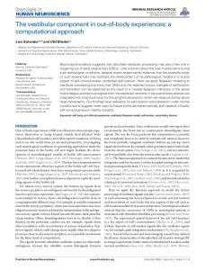
A Computational Expectation Bias The Presentiment Experiments Protocol and results The experiments aim to test the idea that people may have a ”presentiment” of what is going to happen. This presentiment, it is thought, is not necessarily strong enough to reach the conscious level; it is rather thought that a presentiment tends to remain at an unconscious level and that it, consequently, is most properly measured indirectly, preferably using some physiological measure, rather than by means of subjective reports. The physiological measure that has most often been used in presentiment experiments is some measure of electrical skin resistance, or electrodermal activity (EDA), which is generally assumed to be a valid measure of emotional arousal. A typical experiment is conducted as follows. The participant is connected to electrodes, for measurement of EDA, and is seated in front of a computer screen, on which pictures varying in emotional content are to be shown. When the participant is ready to start, he or she pushes a mouse button, telling the computer to start a trial. Each of a predetermined number of trials (typically around 40) is started by the participant pushing the mouse button; this is done when he or she ”feels like it”. Each trial is divided into three periods: (1) Before the picture is shown (e.g., 5 sec) (2) The picture is shown (e.g., 3 sec) (3) After the picture has been shown (e.g., 5 sec) The pictures are of two types: (a) arousing pictures, that is, emotionally activating pictures (for example, pictures depicting violence or sexual motifs) and (b) calm pictures. The pictures shown are selected randomly, with replacement, from a pool. The number of activating and calm pictures need not be the same. In order to avoid, or minimize, habituation, there is most often a larger number of calm pictures than of activating pictures (for example, twice as many calm as activating pictures). The participants´ task merely consists of viewing the pictures as they appear on the screen. In mainstream research, when data are averaged across participants and pictures, this type of protocol normally results in much stronger EDA reactions in response to activating pictures than in response to calm pictures. What Radin found, however, was that stronger EDA reactions were triggered by activating pictures than by calm pictures not only after the pictures had been shown, but also before they were shown. A result of expectation effects? The objection that the above results could be due to expectation effects rather than precognition has been a major theme in the short history of presentiment research. Already in his first paper on presentiment, Radin himself considers this argument, and rejects it (Radin, 1997a). The argument goes as follows. It could be that the participants´ arousal level increases on each trial when a calm picture is shown, right until a trial with a calm picture appears, whereupon the arousal level returns to baseline, increases again on each trial until a new activating picture is shown, whereupon it returns to baseline again, and so forth. This theoretically possible behavior could occur if participants believe that the likelihood of the next picture being activating increases as the number of calm pictures shown since the last activating picture increases (that is, ”the gambler's fallacy”). An example showing how this could lead to the arousal level always being at a peak shortly before an activating picture is presented in Fig. 1.
A Computational Expectation Bias
Fig. 1. The figure shows how expectation effects could lead to an illusionary increased arousal level just prior to the presentation of an activating picture. Dashed vertical lines indicate trials with activating pictures. Calm pictures are shown on other trials.
In a letter to Journal of Scientific Exploration (1998), Radin is criticized by Suitbert Ertel for not having sufficiently convincingly shown why his results could not be explained as an expectation effect, as described above. Later, however, Bierman (1999) furnished a mathematical proof that seemed to demonstrate that, and why, no expectation effect could lead to the results in question. This proof is consistent with a computer simulation (carried out by two of the authors JD and JW) of the behavior illustrated in Fig. 1, involving as many as 10,000 trials instead of the small number (71) depicted in Fig. 1. It turned out that the average arousal level just before an activating picture was almost exactly as high as the average arousal level just before a calm picture. Similar simulations, giving the same results, have been conducted by Bierman and Radin (personal communication). Apparently, then, there is no doubt that, in the long run, the average arousal level will be the same before an activating picture as before a calm picture. As a matter of fact, on second thought, this appears to be self-evident: Since each new picture is statistically independent of the pictures shown earlier (remember that the pictures were sampled with replacement), the average expectation level should be the same before activating pictures as before calm ones. Thinking otherwise would be tantamount to believing that ”the gambler´s fallacy” is not a fallacy after all. As will be shown below, however, the situation is a bit more complicated than one might expect. Puzzling computer simulations In view of what has been said above, the computer simulation in an unpublished study by Radin (1999) is surprising. In this simulation, fifty ”participants” ”observed” a sequence of randomly selected activating and calm pictures (with replacement), the ratio between calm and activating pictures being 2:1. The participants' behavior was exactly the same as that illustrated in Fig. 1. The baseline for arousal was thus set to 0, and on each successive trial, the arousal level was increased by one unit until an activating picture was shown, whereupon the arousal level was reset to 0. The simulation was run for sequences ranging in length from 14 through 112 trials. The results revealed a small, but clear, positive difference between activating and calm pictures, which, however, decreased as the length of the sequence
A Computational Expectation Bias increased! (Somewhat surprisingly, Radin rejected the difference as probably being due to sampling errors.) In order to test the reliability of Radin´s simulation, we have run a similar simulation of our own, involving 50 ”participants”, each one ”being presented with” a number of calm and activating pictures, with a ratio of 1:1 between calm and activating pictures (to match other analyses to be considered later). In order to extend Radin´s simulation so as to include very small sequences, the lengths of the sequences ranged from 2 (instead of 14) through 112 trials. And in order to diminish sampling errors, the ”experiment” was repeated 5,000 times for each sequence length. The results are shown in Fig. 2. The main results, that is, the difference in arousal level between activating and calm pictures prior to each new picture, are represented by the middle curve. The upper and the bottom curves indicate the 95% confidence intervals, and the two broken curves represent ±1.96 standard deviations, calculated over the 5,000 experiments for each sequence length. Fig. 2 shows, beyond any reasonable doubt, that the expectation effect is real. But the figure also shows – just as in Radin´s corresponding simulation – that the effect decreases as sequence length increases; what is more, the figure also seems to demonstrate that the effect – again in agreement with Radin´s simulation – approaches 0 as the sequence length approaches infinity. It may also be noted, in passing, that the two curves representing ±1.96 standard deviations fall within the 95% confidence intervals, indicating that the expectation effects are not normally distributed (had they been, they would have covered the 95% confidence intervals). 1,2 1,0
,8
Bias
,6
,4 Mean dif ,2 2.5% lowest
0,0
2.5% highest
-,2
Mean dif - 1.96 sdev
-,4
Mean dif + 1.96 sdev 2
12
22
32
42
52
62
72
82
92 102 112
Numbers of trials in simulated experiments
Fig. 2. The graph shows the results of a simulation involving 50 ”participants”, each one being presented with sequences of calm and activating pictures in a pool, with a ratio of 1:1 between calm and activating pictures. The middle curve represents the difference in arousal between activating and calm pictures prior to each new picture. The upper and the lower curves indicate the 95% confidence intervals, and the two broken curves represent ± 1.96 standard deviations, calculated over the 5, 000 experiments for each sequence length.
In the simulation presented in Fig. 2, the mean arousal levels preceding arousing or calm pictures were calculated for each individual “participant” separately and before mean
A Computational Expectation Bias differences were calculated. This is not the only possible procedure, however. One alternative is (a) to sum up the arousal values preceding activating and calm pictures, respectively, for each participant and (b) to calculate the mean sum across participants for the respective activating and calm pictures. As far as bias is concerned, this is, in effect, equivalent to calculating the sum of the individual summed arousal levels prior to activating and calm pictures, respectively, since the number of participants is the same for both types of pictures. Another alternative is (a) to merge all the sequences into one single cluster of sequences and (b) to calculate the mean arousal level prior to activating and calm pictures, respectively, for this whole cluster directly, instead of first calculating the means for each individual sequence separately, as in Fig. 2. Replications of the simulation shown in Fig. 2 using these two alternative procedures are shown in Fig. 3. Fig 3A
Fig 3B
6 4
,2
-,2
-2 -4 -6 -8
-,4 -,6
-10 -12-14
,04 ,02
Strength of bias
112
102
92
82
72
62
52
,06 0,00 -,02
112
102
92
82
72
62
52
42
-,06
Number of trials in simulated expe
MeanRefe dif rence line at 0
-,04
Number of trials in simulated expe
Mean 2.5% 2.5% thighe Meanst Mean dif lowes dif - 1.96s dif +dev 1.96sdev
32
112
42
102
22
112
92
32
102
82
12
92
72
22
82
62
12
2
2
72
52
e
62
42
12
52
32
Number ofEnlar trialsgeme in simu nt lated of theexpe rimen ts graph abov
42
22
2
32
,6 ,5 ,4 ,3 ,2 ,1 -,0 -,1 -,2 -,3 -,4 -,5 -,6
Number of trials in simulated expe riments Enlargement of the graph above
22
12
2
Mean 2.5% 2.5% thighe Meanst Mean dif lowes dif - 1.96s dif +dev 1.96sdev
-,0
0
Mean 2.5% 2.5% thighe Meanst Mean dif lowes dif - 1.96s dif +dev 1.96sdev
2
Strength of bias
Strength of bias
,4
8
Strength of bias
,6
14 12 10
Fig. 3. The figure shows two different replications of the simulation shown in Fig. 2. In Graph A, means of summed arousal values prior to activating and calm pictures, respectively, have been calculated across sequences/participants. In Graph B, mean arousal values prior to activating and calm pictures, respectively, have been calculated across stimuli after sequences have been merged into a cluster. riments
riments
As can be seen from Fig 3A, when the sums of individual arousal values are averaged across sequences/participants, there is no bias. As can be seen from Fig. 3B, however, when means are calculated across stimuli for the whole set of sequences without first calculating individual means, there is a bias, although a substantially smaller one than that obtained in Fig. 2. Thus far, our major simulation results can be summarized as follows: In the long run (one subject and 10,000 trials, and extrapolation of the results in Figs. 1 through 3), there is
A Computational Expectation Bias no discernible difference in arousal level between activating and calm pictures, in accord with the fact that each picture is statistically independent of previously presented pictures. But in the long (5,000 experiments with 50 participants) short (say 20, or so, trials) run, there actually is a difference in arousal between activating and calm pictures, unless individual sums (in contrast to means) of arousal values are averaged across participants/sequences (in contrast to stimuli), in which case no bias occurs. Different arousal models Any simulation of real presentiment experiments is, of course, critically dependent on how the arousal level, or, more generally, the expectation about which type of picture is going to be presented on the next trial, changes as a function of previous pictures. Thus far, we have only considered one possible model, depicted in Fig. 1, according to which the arousal level increases linearly as a function of the number of calm successive pictures. An alternative model would be one where arousal grows as a positively accelerated function of the number of calm successive pictures, such as an exponential function. In our view, however, the most realistic model has a sigmoid form. At the beginning of a series of calm stimuli, there is probably no strong expectation, or any expectation whatsoever, that an activating stimulus will be presented on the next trial, meaning that arousal would grow only slowly, or not at all, at the beginning of the series. But as the number of calm successive stimuli increases, it is reasonable to assume that the expectation of the next stimulus being activating would grow increasingly fast, up to some inflexion point at which the curve levels off. In the next major section, however, where the bias will be analyzed more theoretically, we will turn to a simpler model. For convenience, we will use a binary model. In that model, instead of assuming that arousal in a series of calm pictures increases monotonically, as in the above models, arousal increases from 0 to 1 at the first picture in a series of calm pictures and remains at that level until an activating picture resets the level to 0 (see Fig. 4). Although this model is certainly highly simplified, it still captures the essence of the bias. 4,0
Arousal
3,0
2,0
1,0
0,0 1
5
9
13 17 21 25 29 33 37 41 45 49 53 57 61 65 69
Trial number
Fig. 4. The graph shows a simplified, binary model of how expectation effects could lead to an illusionary increased arousal level just prior to presentation of an activating picture. Arousal increases from 0 to 1 at the first picture in a series of calm pictures and remains at that level until an activating picture resets the level to 0.
A Computational Expectation Bias Quantitative estimates of effect sizes An important question to consider is how large the artefacts can be. A precise answer would allow us to estimate the probability that reported psi effects might be explained away by this artefact. As can be seen from the qualitative treatment above, the effect size is dependent on the number of trials that are pooled before one averages. Also, the effect size is dependent on the strategy that subjects use depending on the “history” of past trials. Finally, the effect is dependent on the ratio between the two types of target. Simulations were performed using a “realistic” presentiment experiment, involving 16 subjects and 32 trials per subject. It should be noted, however, that presentiment experiments have been performed with a much smaller number of subjects and that the effects can be expected to be larger for a smaller number of subjects. Simulations were run for two ratio’s: Activating: Calm = 1:1 and 1:2, respectively. First, we tried four models of reasonable strategies, mentioned above: (1) the binary model, (2) the linear model, (3) the exponential model (chosen so as to yield a growth rate of about thirty percent) and (4) the sigmoid model (with an increasing growth rate starting at the fifth trial and a declining growth rate starting at the nineth trial). Each of these models reflects a specific way by which subjects adjust their anticipation as a function of the number of consecutive calm pictures. The observed biases are expressed as a relative effect: Bias = 100 ×
Mean Activating − MeanCalm Mean All
The results of a simulation of about a million of such experiments is shown in Table 1. As can be seen, for both ratios, all four models yield substantial artefacts when averages are calculated per subject, but when subjects are pooled before averaging, the bias becomes extremely small. Table 1: Means and standard deviations of biases from a simulation of four different models and two ratios between activating and calm stimuli.
Averaged per Ss Model
Binary Binary Linear Linear Exponential Exponential Sigmoid Sigmoid
Averaged all pooled
Ratio
Mean (%)
SD (%)
Mean (%)
SD (%)
1:1 1:2 1:1 1:2 1:1 1:2 1:1 1:2
6.39 4.70 12.48 7.07 11.34 22.99 6.39 12.05
1.26 0.95 1.61 0.74 1.86 7.17 0.76 1.26
-0.053 -0.100 0.008 0.002 0.057 0.080 0.020 0.020
1.25 0.97 1.77 0.80 2.10 3.82 1.39 1.39
The question remains if there are no other models that will give larger artefacts. To investigate this, we simulated random models by specifying the anticipation as a function of
A Computational Expectation Bias number of consecutive calm stimuli as coefficients. We assumed throughout that the activation after one or more consecutive activating stimuli was always 0. The values of the coefficients were determined randomly, and after a million of such simulations, the coefficients yielding the largest bias were selected for an extensive test. This method might, of course, just miss a peculiar combination of coefficients (we use 32), because the search space is extremely large. Therefore we used a more systematic “hill-climbing” approach as well: First the largest bias was searched with systematic variation of the first four coefficients and then the next four were systematically explored while holding the first four at the values that generated the largest bias to begin with. There is a small risk that this approach might result in a local maximum with other unobserved maxima. The results of our search for the largest bias resulting from any model are given in Table 2. Table 2: Means and standard deviations arising from search for the largest bias producing model.
Averaged per Ss
Averaged all pooled
Worst Model
Ratio
Mean
Sd
Mean
SD
Random search Systematic search Random search Systematic search
1:1 1:1 1:2 1:2
12.96 26.14 10.78 22.35
2.08 5.16 1.75 3.34
-0.046 0.310 0.012 -0.004
2.14 5.50 1.74 3.38
Apparently the random search method does not work well, but the systematic search gives results that are indeed larger than found with analytical models as show in Table 1. Realizing that, for combinatorial explosion reasons, the systematic search only used the first eight coefficients, it is not impossible that models exist which produce even larger artefacts. In further research the analyses should be extended to models of strategies which take into account the number of consecutive activating stimuli, or any other history; but at this point, analytical methods should probably take over. From the simulation results it can be concluded that for realistic experiments the method of averaging per subject is introducing errors in the order of magnitude of the empirically observed effect or even larger. An argument that actual data show that a specific model does not apply can not be used because, as can be seen from the results, all models do result in measurable bias and thus different subjects might use different models, which will obscure an overall search for a shared model. Nonetheless, these subjects will introduce a bias. On the other hand, it is also clear that pooling all data before averaging is a sound procedure. It is not infallible, however, as indicated by the 0.30 % bias produced by the systematic search for the 1:1 ratio. (All or most published pre-sentiment experiments have pooled the date before averaging.)
A Computational Expectation Bias Theoretical Considerations When the bias stays away As suggested above (Fig. 3A), one way of avoiding the bias is to refrain from calculating mean arousal levels across stimuli and just compare summed arousal units prior to activating and calm pictures – either directly or after averaging across sequences/participants. That no bias appears in this procedure follows inevitably from the fact that the arousal state at any particular point in a sequence is independent of whether the next stimulus is an activating stimulus (A) or a calm stimulus (C). The gambler´s fallacy is a fallacy! However, as will be argued in the discussion, the “just sum” method runs a high risk of leading to Type II errors, that is, a failure to detect any possible real effect. Let us now consider an infinitely long sequence of randomly ordered activating and calm stimuli. The expected number of calm stimuli in such a sequence, E(NC), is half of the total number of stimuli, N:
N 2 = ) C (N E The same is true of the expected number of activating stimuli, E(NA):
N 2 = )A (N E
.
Because stimuli are randomly distributed, half of the calm stimuli will be preceded by another calm stimulus; hence, their preceding arousal values will be equal to one unit. For the same reason, half of the activating stimuli will also be preceded by a calm stimulus, and their preceding arousal values will also be equal to one unit. It then follows that the expected average arousal level prior to a calm stimulus, E(a C), becomes _ and that the expected mean arousal level prior to an activating stimulus, E(aA), also becomes _. Besides revealing the exact values of E(aC) and E(aA) for the binary arousal model, this derivation confirms our previous statement that no bias occurs when a randomly distributed sequence of calm and activating stimuli is infinitely long. In addition to refraining from calculating mean arousal values across stimuli, there is also another method of avoiding the bias. By considering all possible sequences of a given length, one finds that no bias exists when all of them are merged into a single cluster or, in other words, when all participants are “replaced” by one single “super person”. The reason why this happens is the following: Since (i) the total number of A-stimuli is the same as the total number of C-stimuli and (ii) the total sum of arousal units preceding A-stimuli is the same as the total sum of arousal units preceding C-stimuli, the mean arousal level for Astimuli must be equal to the mean arousal level for C-stimuli. It should be pointed out, however, that, in an infinitely long sequence, the overall arousal means for activating and calm pictures will not be equal to the expected values. As can be easily shown, when all possible sequences are merged into a single cluster, the mean arousal level preceding both activating and calm stimuli follows from the expression:
1 − n n 2
,
A Computational Expectation Bias where n is the sequence length. As can be seen from this expression, the mean arousal levels increase continuously from _ in the case of n=2 and continue to approach 0.50 as the sequence length increases. But why, then, do the mean arousal values in a real, finite sequence, or a set of merged real sequences, deviate from 0.50 – the expected value for an infinitely long sequence? This question will be addressed below. Finite versus infinite sequences A real sequence of the type now considered can be thought of as a segment of an infinitely long sequence of randomly ordered successive A- and C-stimuli, associated with arousal units according to the binary model (indicated as 1A or 1C), as illustrated by the sequence ………. . C 1A C 1C 1A C 1A C 1A C 1C 1A A A A ………… Now, if such a sequence is partitioned into smaller sequences, the original sequence may be cut off at four different places: (1) between two C-stimuli, (2) between one C-stimulus and a following A-stimulus, (3) between an A-stimulus and a following C-stimulus, and, (4), between two A-stimuli. This is indicated by the vertical bars in our illustrating segment: ………. . C 1A C |C A C |A C 1A |C 1C A | A A A ………… The first two types of cuts have the effect of eliminating arousal units; the first cut eliminates an arousal unit preceding a C-stimulus and the second cut an arousal unit preceding an A-stimulus. Both these effects lead to a general reduction of the ratio between the number of arousal units preceding a given type of stimulus (A or C) and the total number of stimuli of the same type. The two other cuts have no such consequences and are thus irrelevant as far as the number of arousal units is concerned. Thus, in forming particular sequences, by cutting the connection between a C-stimulus and the following C- or A-stimulus, one reduces the total number of arousal units preceding A- or C-stimuli as compared to the total number of Aor C-stimuli. The smaller the sequences formed by the cuts, the larger the amount of the reduction. Why does the bias appear and why is it dependent on sequence length? To get an intuitive understanding of why and how the bias arises, it is useful to consider all possible sequences of the shortest possible length, two stimuli. There are four possible such sequences: CC, CA, AC and AA, corresponding to an experiment with four participants, each one being presented with two stimuli. The expectation/arousal effects for the four stimulus pairs are shown in Table 3. As can be seen from Table 3, the average arousal level prior to activating stimuli (0.33) is larger than the average arousal level prior to calm stimuli (0.17). Why is it so? We may first note that the stimulus pairs CC and CA differ from the stimulus pairs AC and AA in that the two former stimulus pairs are both associated with increased arousal levels, while the two latter stimulus pairs are not. We may further note that some of the four stimulus pairs differ from each other with respect to number of C-stimuli, nC, and the number of A-stimuli, nA; the CC-pair consists of two C-stimuli but no A-stimulus; both the CA-pair and the AC-pair consist of one A- and one C-stimulus; and the AA-pair, finally, is composed of two A-stimuli.
A Computational Expectation Bias Table 3. Analysis of expectation/arousal effects for activating and calm stimuli for the four possible sequences consisting of two stimuli.
Stimuli Activating
Calm
Sequences
Sum(aA)
nA
Mean(aA)
Sum(aC)
nC
Mean(aC)
C 1C C 1A A C A A
0 1 0 0
0 1 1 0
1 0 0
1 0 0 0
2 1 1 0
1/2 0 0 -
Sum Mean
1 0.25
4 1
1 1/3=.33
1 0.25
4 1
1/2 1/6=.17
“1”= one arousal unit preceding an activating or a calm stimulus; Sum(aA)=sum of arousal units preceding activating stimuli; nA=number of activating stimuli; Mean(aA)=mean of arousal units preceding activating stimuli; Sum(aC)=sum of arousal units preceding calm stimuli; nC=number of calm stimuli; Mean(aC)=mean of arousal units preceding calm stimuli.
The fact that the bias occurs is, as can be seen, attributable to the difference between the two arousal generating stimulus pairs, CC and CA. The first C in the CC-pair and the single C in the CA-pair are both generating the same arousal magnitude, one unit. But there is only one A-stimulus in the CA-pair, while there are two C-stimuli in the CC-pair. As a consequence, the mean of the arousal magnitude created by the first C-stimulus in the CA-pair (1/1) becomes higher than the mean of the arousal magnitude created by the first C-stimulus in the CC-pair (1/2). And since neither the single A-stimulus in the AC-pair nor the first A-stimulus in the AA-pair generates any arousal at all, the overall mean arousal level prior to A-stimuli (0.33) becomes larger than the overall mean arousal level prior to C-stimuli (0.17). This explanation will later be worked out in more detail and generalized to longer sequences. But before that we will take a closer look at the relation between the magnitude of the bias and sequence length. Table 4 shows the means of the individual average arousal magnitudes preceding activating and calm stimuli, respectively, as well as the corresponding values of the bias for sequences ranging in length from two through twelve stimuli. For activating stimuli, the total mean increases rapidly, reaching the expected value for an infinitely long sequence, 0.50 (disregarding further decimals), already at the sequence length of seven stimuli. For the calm stimuli, by contrast, the total mean increases more slowly, reaching an upper limit of 0.42 for the present range of sequence lengths. Disregarding the increment in the size of the bias when the sequence length increases from two to three stimuli, the bias diminishes continuously as the sequence length increases. In the analyses leading to the results shown in Table 4, comparisons between arousal levels for activating versus calm stimuli were made on the group level; that is, before mean differences were calculated, the mean arousal levels prior to activating and calm stimuli were calculated across participants. But our original simulation in the previous section (Fig.2) was run on the individual level; that is, before the final mean differences were calculated, mean differences were calculated for each individual “participant” separately (giving a higher statistical power than a corresponding analysis at the group level, as noted before).
A Computational Expectation Bias Table 4. Means of individual mean arousal levels preceding activating and calm pictures and corresponding bias values for sequences ranging in length from two through twelve stimuli.
Stimulus Sequence Length (No. of Stimuli)
Activating
Calm
Bias
2 3 4 5 6 7 8 9 10 11 12
0.33 0.43 0.47 0.48 0.49 0.50 0.50 0.50 0.50 0.50 0.50
0.17 0.24 0.28 0.32 0.34 0.36 0.38 0.39 0.40 0.41 0.42
0.17 0.19 0.18 0.17 0.15 0.14 0.12 0.11 0.10 0.09 0.08
Table 5 shows such a within subjects analysis for the same sequence length as in Table 1, that is, two stimuli. In this table, the CC-sequence and the AA-sequence in Table 3 (the uppermost and the bottom sequences) have been dropped. The reason is, of course, that in a within subjects analysis of the present type, not only undefined values have to be excluded, that is, the average arousal level preceding A-stimuli in the sequence consisting solely of Cstimuli and the average arousal level preceding C-stimuli in the sequence consisting solely of A-stimuli, but both these sequences must be excluded altogether, so that each sequence consists of at least one A-stimulus and at least one C-stimulus. Table 5. Within subjects analysis of expectation/arousal effects for activating and calm stimuli for the two possible sequences consisting of two stimuli.
Stimuli Sequences
Activating Sum(aA) nA
Mean(aA)
Calm Sum(aC) nC
Mean(aC)
Mean(aA)Mean(aC)
C 1A AC
1 0
1 1
1 0
0 0
1 1
0 0
1 0
Sum Mean
1 1/2
2 1
1 1/2
0 0
2 1
0 0
1 1/2
“1”= one arousal unit preceding an activating or a calm stimulus; Sum(aA)=sum of arousal units preceding activating stimuli; nA=number of activating stimuli; Mean(aA)=mean of arousal units preceding activating stimuli; Sum(aC)=sum of arousal units preceding calm stimuli; nC=number of calm stimuli; Mean(aC)=mean of arousal units preceding calm stimuli.
A comparison between Table 3 and Table 5 shows the effect of excluding the uppermost and the bottom sequences in Table 3: The mean of the average individual arousal levels preceding activating stimuli has increased from 0.33 to 0.50 (the expected value for an infinitely long sequence!), whereas the mean of the average individual arousal levels prior to calm stimuli has decreased from 0.17 to 0.
A Computational Expectation Bias Table 6 replicates Table 4 using within subjects analyses instead of group level analyses. Table 6 thus shows the means of the individual average arousal levels preceding activating and calm stimuli, respectively, as well as the corresponding values of the bias, using within subjects analyses for sequences ranging in length from two through twelve stimuli. We may first note that the mean of the average individual arousal levels preceding activating stimuli now is equal to 0.50 throughout, and not only for sequences exceeding six stimuli, as in Table 4. This is an important finding. It shows that the previously demonstrated deviations from 0.50 in our group level analyses can altogether be attributed to one single sequence: the one consisting solely of activating pictures. Thus, the earlier deviations from 0.50 arose as a consequence of this particular sequence being included in the calculation of the mean of the average individual arousal levels preceding activating stimuli, thereby decreasing the overall mean as compared to the present analysis. This, in turn, explains why the total mean approached 0.50 so rapidly: Since only one of all possible sequences is solely composed of activating stimuli, this sequence becomes an increasingly smaller proportion of the total set of sequences as sequence length – and hence the number of possible sequences – increases. Table 6. Means of individual mean arousal levels preceding activating and calm pictures and corresponding bias values using within subjects analyses for sequences ranging in length from two through twelve stimuli.
Type of Stimulus Sequence Length (No. of Stimuli)
Activating
Calm
Bias
2 3 4 5 6 7 8 9 10 11 12
0.50 0.50 0.50 0.50 0.50 0.50 0.50 0.50 0.50 0.50 0.50
0.00 0.17 0.25 0.30 0.33 0.36 0.38 0.39 0.40 0.41 0.42
0.50 0.33 0.25 0.20 0.17 0.14 0.12 0.11 0.10 0.09 0.08
Thus, in a within subjects comparison between activating and calm stimuli using the present model, only the calm stimuli deviate from the behavior in an infinitely long sequence. Through simulations, we have found that, in such a comparison, the total mean of the arousal levels preceding calm stimuli, TM, is related to sequence length, SL, by the simple equation
2 2 − × SL SL =
TM
.
But how is it, then, that the bias does appear and decreases as sequence length increases? We have already suggested that the C-stimuli, and not the A-stimuli, are responsible for the bias. In all sequences with at least one A-stimulus and one C-stimulus, the
A Computational Expectation Bias ratio between the number of arousal units preceding A-stimuli and the total number of Astimuli is exactly the same as in an infinitely long sequence (see Tables 4 and 6). In order to understand how the C-stimuli give rise to the bias, it is useful to make a distinction between two different “roles” that a C-stimulus can play: (a) as a “sender” of an arousal unit to the next stimulus in the sequence and (b) as a “receiver” of an arousal unit from the previous stimulus. The first C-stimulus in a (partial or complete) sequence consisting solely of C-stimuli only plays the role of a sender of an arousal unit, not that of a receiver. By contrast, all other stimuli in the sequence act both as a sender and as a receiver (except for the last C-stimulus in a complete sequence, which only acts as a receiver). Here (bold text) are some examples of the type of sequence we have in mind: C1CAAC1CACAC…… C1C1CAC1CACAC…… ACAC1CACAC1CA…. AAAC1C1C1C1C1CAC1CA.. C1C1C1C1C1C1C1C1C1C1C1C1C1C1C1C1C In such sequences, there is always one stimulus more than there are arousal units – the stimulus initiating the sequence, which only acts as a sender of arousal, not as a receiver. This means that, in calculating the mean arousal level preceding calm stimuli for a complete sequence (a participant), the denominator always consists of at least one stimulus more than the number of arousal units. Generalizing from the simple example in Table 3, with only two stimuli in each sequence, this means that bias will occur. But C-stimuli that are followed by one or several other C-stimuli do not always have the same impact. A C-stimulus that initiates a long sequence of C-stimuli gets a smaller weight than a C-stimulus that initiates a shorter sequence. Whereas, for example, the mean arousal level for the sequence CCCC becomes _, the mean arousal level for the shorter sequence CCC becomes only 2/3. Thus, the strength of the bias diminishes as the number of C-stimuli initiating (partial or complete) sequences of C-stimuli diminishes relative to other C-stimuli. This relationship explains why the bias decreases as sequence length increases. When sequence length is relatively short, sequences consisting solely of C-stimuli are necessarily relatively short. But as sequence length increases, sequences consisting solely of C-stimuli will, on the average, become longer, since an increment of the sequence length permits – and necessitates – that longer sequences of C-stimuli will be formed. This, in turn, means that Cstimuli followed by one or several other C-stimuli will, on the whole, be reduced in number relative to other C-stimuli. As a consequence, the average of the mean arousal levels preceding C-stimuli will continuously approach 0.50, the value in an infinitely long sequence, and, accordingly, the bias will continuously be reduced. Incomplete merging of sequences We have earlier noted that the bias vanishes altogether when all possible sequences are merged into a single cluster. But we have also noted that the bias still remains when only a sample from the complete set of possible sequences is analyzed (Fig. 3B). It is therefore reasonable to assume that the bias decreases gradually as a function of the size of the sample from all possible sequences. In the following, we will show that this is true. That the bias gradually diminishes when different sequences of a given length become merged into increasingly larger clusters before mean arousal values are calculated follows, as we will see, from the fact that the bias ceases to exist when all possible sequences of a given
A Computational Expectation Bias length are merged into a single cluster. To show this, we return to the set of sequences consisting of only two stimuli: C1C C1A AC AA. If the four different stimulus pairs are combined in pairs, in all possible orders (corresponding to sampling with replacement), we will get 42=16 different pairs of stimulus pairs. Each of these combinations corresponds to a separate experiment involving two participants, each of whom is presented with two stimuli. The bias is calculated by averaging the mean arousal levels preceding activating and calm stimuli, respectively, across the 16 possible experiments, wherein the two sequences in each experiment have been merged into one cluster. If the four different stimulus pairs, instead of being combined in pairs in all possible orders, are combined in triples in all possible orders, we will get 43=64 different triplets of stimulus pairs, each triplet corresponding to a separate experiment involving three participants, each of whom is presented with two stimuli. As in the case of pairwise combinations of sequences, the bias is calculated by averaging the mean arousal levels preceding activating and calm stimuli, respectively, across all possible different experiments (64) with the three sequences in each experiment being merged into one cluster. Table 7 shows how the bias decreases as the number of sequences in each experiment increases from one (separate sequences) through four – the merging of all four sequences into a single cluster. As can be seen, the activating and the calm stimuli approach the unbiased value of 0.25, though from “opposite directions” – the former from higher values and the latter from lower values – as the number of sequences being merged increases from one through four. Specifically, (at least in this example) the bias decreases linearly with the number of sequences. Table 7. Total means of average arousal levels prior to activating and calm stimuli, respectively, and the corresponding bias for the sequence length of two stimuli for varying number of sequences being merged into one cluster.
Stimuli Number of Sequences
Activating
Calm
Bias
1 2 3 4
0.33 0.31 0.29 0.25
0.17 0.19 0.21 0.25
0.16 0.12 0.08 0.00
But how can we explain the fact that the size of the bias diminishes as a function of the number of sequences being merged? One way of doing this (there are probably other ways as well) is to regard the set of all possible sequences of a given length as a population of sequences and subsets of this set, that is, clusters of sequences or the single sequences themselves, as samples from this population. For the sequence length of n stimuli, the population consists of 2n sequences. This means that 2nm different samples with m sequences in each sample can be drawn from the population.
A Computational Expectation Bias A particular measure of the individual sequences – for instance, the mean arousal level preceding activating stimuli, Mean(aA), or the mean arousal level preceding calm stimuli, Mean(aA) – can now be regarded as a sample property. How well a given sample property matches the corresponding property of the population is, as is well known, dependent on the size of the samples. By virtue of the law of large numbers, as the size of the samples increases, the match between the samples and the population will increase, due to differences between elements within samples being increasingly counterbalanced. In Table 5, this is reflected by the fact that Mean(aA) and Mean(aC) gradually approach 0.25 – the value of Mean(aA) and Mean(aC) for the total set of sequences – as the size of the samples increases from m=1 (no merging at all) through m=3 (merging of the individual sequences in triples).
Discussion There is no doubt that the presentiment experiment could be afflicted by a potential statistical bias, based on an expectation effect: an effect of the expectation that the likelihood of an activating stimulus being presented increases with the number of previous consecutive calm stimuli – that is, a variant of the ”gambler´s fallacy”. It is also clear, though, that the bias decreases as the length of the sequence increases and is non-existent in the theoretical case of an infinitely long sequence, consistent with the fact that stimuli are statistically independent of each other. Using a simplified expectation model (Fig. 4), we have been able to explain – though only in a rather informal manner – why the bias appears and why it is dependent on the sequence length. (For a more formal approach to the present bias, see Jiri Wackermann´s2 paper on pages x-y of this volume.) Basically, the bias and its dependency on sequence length are attributable to the occurrence of “chains” of calm stimuli. When means of arousal units prior to calm stimuli are calculated for individual sequences, the first stimulus in such a chain enters into the calculations even though it is not preceded by any arousal itself. This will lead to a reduction in the mean arousal prior to calm stimuli as compared to the mean arousal prior to activating stimuli. But as the sequence length increases, the effect will diminish, due to the reduced importance of the first calm stimulus in a series of such stimuli. When data are analyzed on the individual level, the present bias poses a serious threat to any presentiment experiment, due to its large effects (see Tables 1 and 2). Even though some statistically significant experimental effect would be larger – or even much larger – than the effect predicted for some realistic expectation model, or an estimated maximal effect for any model, we do not know to what extent the bias has “helped” the results to reach statistical significance. However, when data are pooled across subjects before means are calculated, the situation is different. It is true that the bias remains unless all possible sequences have been included and are evenly distributed across participants (which, in practice, is impossible using the standard design), but the expected effect of the bias was found to be extremely small for 2
Starting from different experiments, Jiri Wackerman and our group have identified and investigated the present bias independently and without knowledge of each other´s work. JW:s approach is analytical, whereas ours is computational. Thus, the two approaches complement each other. We do not know whether the bias can be found in previous research. We do know, however, that it has gone unnoticed by all, or the vast majority of, experimental researchers, both within and outside parapsychology.
A Computational Expectation Bias various reasonable models of expectation growth (see Table 1). Nevertheless, pooling data before averaging is not an infallible method. Moreover, even if one is willing to assume that the bias in reality is extremely small and therefore cannot be mistaken for a genuine effect, the effects of the bias are still disturbing, mainly because they render any statistical test difficult or impossible to perform. As an alternative to reducing the effect of the bias by pooling data across sequences, one might find a strategy that does not produce any bias at all. Such a strategy was, indeed, suggested previously in this paper. It is based on the fact that no bias occurs when sums instead of means of individual arousal levels are considered. The corresponding strategy is simply to use the unbiased sums instead of the biased means in comparing arousal levels prior to activating versus calm stimuli. As already suggested, however, there is a drawback also to this strategy: Since the relative number of activating and calm stimuli vary from one participant to another, due to sampling fluctuations, a possible true presentiment effect runs the risk of being obscured by the random effects of unequal numbers of activating and calm stimuli. It is true that the hypothetical presentiment effect might be strong enough to withstand this effect, but there is no good reason to believe a possible presentiment effect to be particularly strong. It is also true that sampling effects can be reduced by increasing sequence length, but sequences can obviously not be made too long without jeopardizing any possible presentiment effect, due to fatigue or reduced motivation on the part of the participants. Nevertheless, the strategy now considered cannot be definitely rejected. An alternative strategy has been suggested by James Spottiswoode (personal communication). This strategy attempts to avoid the bias by using methods of data collection and data analysis that make the data immune to the bias. This is assumed to be accomplished by presenting stimuli at irregular, instead of fixed, time-intervals, and analyzing the change of the response instead of the response itself. Although this is an interesting possibility, some assumptions behind this strategy (for example, that the change of the response is not dependent on the level of the response) need to be investigated. In a sense, the final strategy suggested here is by far the soundest one. Like the “just sum” strategy considered above, it is based on the idea of avoiding calculating means of arousal values across stimuli for separate individuals or samples of individuals. Based on the fact that no bias occurs when all possible sequences are merged into a single cluster, all these possible sequences are entered into the experiment. This means, however, that stimuli as such cannot be randomly chosen; instead, all the possible sequences are randomly distributed across participants. The point is, of course, that in the resulting set of data, the total number of activating and calm pictures will be the same. However, on some conceptions of precognition, such as the occurrence of “timereversal”, predetermining stimulus orders might be an inadequate method, because randomization does not occur in real time, even though the assignment of sequences to subjects can be done in real time. Unfortunately, there are also practical limitations to the present strategy. One is that the sequence length must be very short so as not to give rise to a prohibitory number of different sequences; a sequence length of five stimuli or so is probably maximum. In terms of the total number of trials, however, this limitation can be compensated for by using a large number of participants – one or several participants for each particular sequence. Unfortunately, however, the present strategy cannot be used for re-analyzing old presentiment data, where only samples of sequences are used. Another practical problem is that the experimenter is not allowed to have any contact whatsover with the participants. The statistical bias considered in this paper is certainly not unique to the presentiment experiment, but may potentially occur in many different experiments, both within and outside
A Computational Expectation Bias parapsychology. Experiments that are potentially vulnerable to this bias are, as far as we can see, characterized by the following five properties: (1) There is a fixed number of types of targets (for example the different numbers of eyes in dice throwing), instances of which are randomly presented to the participant, with or without replacement. (There is nothing special about just two target types.) (2) Feed-back is given after each trial; that is, the participant is informed as to whether the response was correct. (3) The different target types are associated with expectation functions that differ from each other in a relevant way (which has to be worked out for particular types of experiments.) (4) The dependent variable is a set of responses that are systematically (but not necessarily monotonically) related to the different expectation functions. (There is nothing special about EDA as an indicator of expectation.) (5) Means, instead of sums, of responses are calculated for each target type and participant (or sample of participants). At the present time, we do not know how many previous ESP experiments satisfy all of the five criteria – or if there exist any that do. In any case, it is important to re-consider as many previous ESP experiments as possible to ensure that none of them have been affected by the present bias. Similarly, the various meta-analyses of different types of ESP experiments that have been carried out during the past decades (see, e.g., Radin, 1997b) should be re-considered to discover whether any of the positive findings might be accounted for by the present bias. Doing so would seem particularly urgent in view of the fact that very small effects may result in significant overall results, due to the large amount of data involved. That this particular bias could in fact have occurred in some previous ESP experiments is suggested by an extensive meta-analysis on “forced choice” precognition experiments conducted by Charles Honorton and Diane Ferrari (1989). There was one single moderator variable discriminating successful from unsuccessful experiments: the occurrence versus nonoccurence of feedback. Although this finding could, of course, be interpreted differently, it does suggest that the present bias could account for the fact that only experiments using feedback gave positive results. Outside parapsychology, there are, most notably, several areas within psychology where experiments that are formally of the same type as Radin´s presentiment experiment have been performed. Among these areas are, for example, psychophysiology, attention, memory and learning. Again, such experiments should be re-considered, to ensure that the present bias was not responsible for the results. The present paper has been exclusively concerned with the case of randomization without replacement, or open deck randomization. However, in mainstream psychology, closed deck randomization is much more common than open deck randomization. This means that, on top of the expectation effect considered in this paper, which properly may be regarded as a numerical bias attributable to faulty calculations rather than to expectations per se, there is another, “true” expectation effect. The combination of the two effects may by quite dramatic. Could the present bias somehow be utilized for making any useful predictions, such as predicting gambler´s performance at the roulette table by means of EDA measures? The answer to this question is definitely “No”. The reason is simple: the bias is basically concerned with the relation between expectations, on the one hand, and the relative number of different types of targets, on the other hand, and not with foreseeing future events. In other words, knowing how expectations tend to be formed on the basis of previous stimuli cannot be used to predict the correctness of these expectations, only to predict how the expectations become “normalized” when means of expectations prior to different types of stimuli are calculated. But this feat is not in any way tantamount to outwitting chance; that is, to
A Computational Expectation Bias predicting performance in terms of the total number or intensity of correct expectations about alternative future events.
References Bierman, D. J. (1999). Sequential patterns cannot explain anomalous anticipatory physiological behavior, A proof. Web-article: http://www.psy.uva.nl/resedu/pn/PUBS/BIERMAN/1999/proof.html Bierman, D. J. (2000). Anomalous baseline effects in mainstream emotion research using psychophysiological variables. Proceedings of Presented papers: The 43rd Annual Convention of the Parapsychological Association, 34-47. Bierman, D.J. and Radin, D.I. (1997). Anomalous anticipatory response on randomized future conditions. Perceptual and Motor Skills, 84, 689. Bierman, D. J. & Radin, D. I. (1998): Conscious and anomalous non conscious emotional processes: A reversal of the Arrow of Time? In: Toward a science of consciousness, TUCSON III, MIT Press, 1999, 367-386. Ertel, S. (1998). Comments on Dean I. Radin’s ”Unconscious perception of future emotions: An experiment in presentiment” (Letters to the editor), 12 (3), 469-470. Hayes, N. (2000). Foundations of psychology (third edition). London: Thomson Learning. Honorton, C. & Ferrari, D.C. (1989). Future telling: A meta-analysis of forced-choice precognition experiments, 1935-1987. Journal of Parapsychology, 53, 281-308. Radin, D. I. (1997a). Unconscious perception of future emotions: An experiment in presentiment. Journal of Scientific Exploration, 11 (2), 163-180. Radin, D.I. (1997b) The Conscious Universe. San Francisco: HarperEdge. Radin, D. I. (1999). Evidence for an anomalous anticipatory effect in the autonomic nervous system. Draft (http://www.boundaryinstitute.org/articles/presentiment99.pdf).