David Connah, Stephen Westland, and Mitchell G.A. Thomson. Colour & Imaging Institute. University of Derby, United Kingdom. Abstract. A computational model ...
IS&T/SID Ninth Color Imaging Conference
A Computational Model for the Design of a Multispectral Imaging System David Connah, Stephen Westland, and Mitchell G.A. Thomson Colour & Imaging Institute University of Derby, United Kingdom Abstract
dimensional in their color content. However, although the mathematics underlying potential solutions for multispectral imaging is well understood the relative merits of these solutions for practical color imaging are less well understood. This manuscript describes research that is underway to develop a computational model of multispectral color imaging that will be used to investigate the impact of design features on the effectiveness of a multispectral imaging system.
A computational model of a multispectral imaging system was constructed and used to simulate the recovery of the spectral reflectance of surfaces imaged by the system. The model allows parameters such as number of sensors, sensor spectral sensitivity and quantization noise to be evaluated in terms of their effect on the accuracy of recovery. A set of 1269 Munsell surface reflectance factors were used to test the model. The recovery process employs a linear system whereby spectral reflectance functions are represented by a small number of basis functions. The results show that increasing the number of sensors in the system or increasing the number of basis functions in the linear model does not necessarily increase recovery performance. However, in general, error does monotonically decrease with increasing sensor number when the number of basis functions used in the linear model is allowed to vary independently of sensor number. These performance aspects of the system are closely correlated with the condition number of the solution matrix.
Multispectral and hy Perspectral Imaging Traditional trichromatic imaging system capture three signals R, G and B at each pixel location corresponding to the activations of three color channels. The RGB responses can be expressed discretely by the following equations,
R = ∑ r (λ ) E (λ )S (λ ),
G = ∑ g (λ ) E (λ )S (λ ),
(1)
B = ∑ b(λ ) E (λ )S (λ ),
Introduction where r, g and b are the channel sensitivities, E is the spectral power distribution of the light source, and S is the spectral reflectance of the surface being imaged, each as a function of wavelength λ. In this, and subsequent representations, we consider only the case for a single pixel. Equation 1 can be conveniently expressed as a linear system in matrix notation (assuming that spectral properties are specified at 31 intervals in the visible spectrum 400-700 nm) thus,
Conventional color imaging using trichromatic imaging systems suffers from two problems which can inhibit successful color management of the image. The first of these problems is that the image captured is device dependent. That is, the image is specified in terms of the primaries (usually RGB) of the capture device. This problem can be overcome by transforming the image into a suitable device-independent color space such as CIE XYZ or sRGB. The second problem is that the image captured is illuminant dependent. If the image is captured under a particular light source (for example, corresponding to CIE illuminant D65) and subsequently reproduced for view under the same light source then the illuminant dependency may not be a problem. The need for more flexible colormanagement strategies has driven research methods towards the design of multispectral imaging systems that use more than three color channels1,2. A further motivating force for the development of multispectral imaging is the emergence of multispectral image reproduction systems3 that would be best exploited by images that are inherently more than three
p = Gs,
(2)
where p is a 3×1 row matrix of the camera response, G is a 3×31 matrix representing the product of the camera sensitivity of each channel with the light source, and s is a 31×1 row matrix representing the reflectance of the surface4. In conventional trichromatic imaging the camera responses p only are recorded. However, consideration of Equation 2 shows that it is possible to recover the spectral reflectance of the surface s from the camera responses by rearranging Equation 2 to yield
130
IS&T/SID Ninth Color Imaging Conference
s = G-1p.
where si are the basis functions of the linear system and ωi are the weights for a particular sample S. Substitution of Equation 4 into Equation 3 allows the recovery of the weights ωi that allow an approximate recovery of the reflectance spectrum. Although in principle a multispectral imaging system with 6 channels can recover six-dimensional estimates of surface reflectance spectra, such an analysis does not take into account the wavelength properties of these channels. For example, a system with channels whose spectral sensitivities are highly correlated with each other will not extract as much useful information as a similar system whose spectral sensitivities are orthogonal. Also, what effect does the wavelength of maximum sensitivity for each channel and the spectral profile of each channel have on the accuracy of the system in terms of recovering spectral reflectance factors? These are the questions that we address using our computational model.
(3)
The inverse matrix G-1 can be computed easily but, since the rank of G is three at most, estimates of s obtained from Equation 3 are not likely to be accurate if s is defined at 31 wavelengths. Ideally we would like the matrix G to be square, but this could only be achieved by reducing our estimate of spectral reflectance to 3, or by increasing the number of channels to 31, or more generally by matching the number of channels to some appropriate dimensionality of surface reflectance factors. The obvious question is what is the minimum number of sensors that we can use to obtain reliable estimates of surface reflectance? The reflectance spectra of most natural and manufactured surfaces are known to be smooth functions of wavelength. Certainly if we used 31 channels then we would expect to be able to recover the reflectance spectra of such surfaces exactly. An imaging device with 31 narrowband channels could be called an imaging spectrophotometer. This type of imaging, where the spectral properties of the image are effectively measured – as opposed to estimated – is also referred to as hyperspectral imaging. However, reasonable estimates of reflectance can be obtained with as few as six channels because the reflectance spectra of surfaces are highly constrained. Whereas hyperspectral imaging refers to an imaging device with a large number of channels and which effectively measures the spectral properties of the surfaces, multispectral imaging refers to an imaging device with a relatively small number (but usually greater than 3) of channels and which estimates the spectral properties of the surfaces in the scene.
Experimental The camera model is an ideal image-capture system based upon a simple mathematical model of the interactions between surfaces, light sources, filters and the camera sensitivities. This model assumes that the camera is a completely linear system thus Pi = ∑ p i (λ ) E (λ ) S (λ ) , i = 1, 2…, N, and λ= 400, 410, 420, … 700 nm.
Here Pi is the output of the ith channel, pi is the sensitivity of the ith channel as a function of wavelength and E(λ) and S(λ) are the spectral power distribution of the illuminant and the spectral reflectance function of the surface. The sensors are always assumed to be Gaussian functions of wavelength, characterised by variable half-widths and wavelengths of peak sensitivity. They are normalised such that the integral of each sensor over the visible spectrum is exactly 1. Reflectance recovery is carried out using a linear modelling approach to derive a set of basis functions from a set of reflectance spectra. The basis functions were derived from a singular value decomposition (SVD) of a matrix whose columns represent the reflectance spectra for 1269 Munsell surfaces9. The result of the SVD is a set of ordered basis vectors for the reflectance set. They are ordered such that those vectors which account for the most variance take precedence. Any given reflectance function can be described as the weighted sum of the set of basis vectors (see equation 4). Expressed in matrix form this gives
Estimates of Reflectance Constraints The statistical properties of reflectance spectra for natural surfaces have been extensively studied. It is known that a linear model with as few as six parameters can account for greater than 98% of the variance for any particular data set5. More recently, several studies of manufactured surfaces such as plastics and painted materials (including the Munsell set of surfaces) have shown that their reflectance spectra are similarly constrained6-8. The smoothness of reflectance spectra can also be expressed in terms of the functions being bandlimited in wavelength space with an upper band limit of about 0.015 cycles / nm. The natural smoothness of most reflectance spectra suggests that about 6 channels should be sufficient to obtain reasonable estimates of the reflectance properties of a scene. The redundancy in spectral reflectance measurements thus allows them to be represented by a linear model with a small number of parameters. For example, assuming 6 channels, we could write
S ≈ ∑i ω i si , for i = 1, … 6
(5)
p = GBw
(6)
where B is a 31×31 matrix whose columns are the basis vectors, and w is a 31×1 column vector whose values are the weights of the basis functions. This problem is still intractable while the dimension of p is less than the
(4)
131
IS&T/SID Ninth Color Imaging Conference
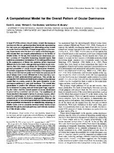
The effect of adding random sensor noise is illustrated by Figure 3 where it can be seen that performance is deteriorated for all sensor numbers but the deterioration is worst for illuminants F11 and A.
dimension of w, but by reducing the number of basis functions used in the approximation of reflectance, the matrix L = GB becomes closer and closer to being square. By using the same number of basis functions as there are sensors, L becomes square and inverting L gives an approximate solution to the original equation.14 Thus p = Lw
(7 )
w = L-1p
(8)
7
6 A 5
and
D65 F11
4
Bw ≅ s.
(9)
Constant
3
2
The resulting reflectance Bw can only be an approximation to s because we have reduced the number of basis functions used in the linear model (Equation 6). In order to simulate more realistic imaging conditions it is necessary to introduce noise into the equations. The approach adopted here is to incorporate a variable random component e into the sensor response, i.e. Pi = ∑ pi (λ )E(λ )S (λ ) + ei .
1
0 3
4
5
6
7
8
9
10
Number of sensors
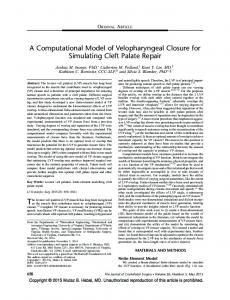
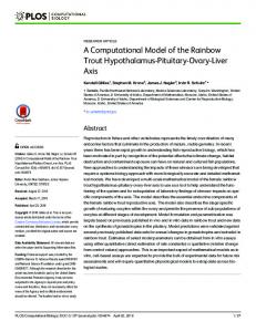
Figure 1: DE as a function of number of sensors for CIE illuminants A, D65, F11 and an illuminant with a uniform spectral power distribution.
(10) 3 Sensors 4 Sensors 5 Sensors 6 Sensors 7 Sensors 8 Sensors 9 Sensors 10 Sensors
4.5
It is also necessary to consider quantization noise, which was simulated by rounding the sensor responses to 8-, 10- and 12-bit accuracy.
4 3.5 3
Results
2.5 2
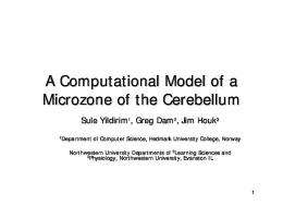
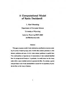
The performance of the system is quantified by the CIELAB ∆E color difference under D65 between the true reflectance spectrum and the recovered reflectance spectrum for each sample in the dataset. Figure 1 shows the ∆E error obtained using four different illuminants in the model. The number of sensors varies between 3-10 in Figure 1. The number of basis functions was set to equal the number of sensors in each case. As the number of sensors is increased so the half-width of each sensor decreases. This ensures that the sensors retain the same mutual orthogonality. However, it means that sensor half-width and number of sensors are confounded. The figure shows that increasing the number of sensors (and consequently increasing the number of basis functions) does not necessarily improve performance. In order to untangle the effect of changing the halfwidth and the number of the sensors, the experiment was repeated for different half-widths independent of number of sensors. Figure 2 shows the ∆E error plotted against sensor half-width for 3-10 sensors. There are two main features to note. Firstly, with the exception of the case where there are three sensors, the ∆E error generally increases with increasing sensor half width. Secondly, the results for six sensors are markedly worse than for five and seven sensors (there is also some evidence of this in Figure 1).
1.5 1 0.5 0 10nm
30nm
50nm
70nm
90nm
110nm
130nm
150nm
170nm
190nm
Sensor half width
Figure 2: DE reconstruction as a function of sensor half width for 3 to 10 sensors 35 30 A D65
25
F11 Constant
20 15 10 5 0 3
4
5
6
7
8
9
10
Number of sensors
Figure 3: Reconstruction performance as a function of sensor number for four different illuminants. Results are shown in the presence of random sensor noise.
132
IS&T/SID Ninth Color Imaging Conference
Table 1: Condition numbers of the solution matrix L for different model parameters. Sensor half-width No. Sensors 30nm 70nm 110nm 3 1.28 1.42 2.04 4 1.57 1.96 4.26 5 1.85 2.87 9.85 6 7.89 21.62 198.00 7 3.19 6.69 53.47 8 8.39 27.94 437.81 9 5.80 20.55 815.91 10 31.09 48.96 1848.36
14 8 bit
12
10 bit 12 bit
10
Un-quantised
8 6 4 2 0 3
4
5
6
7
8
9
10
Number of sensors
Figure 4: Reconstruction error plotted against sensor number for four quantization regimes (half-width = 110nm, spectrally uniform illuminant)
Table 1 shows the condition number10 of the solution matrix L, computed by L×L-1, as a function of both sensor half-width and number of sensors in the case of a spectrally uniform illuminant. The condition number tends to rise with both sensor number and sensor half-width. It is also clear that the condition number rises abnormally for six sensors, which is likely to have a role in the larger errors observed when using six sensors (see figures 1, 2 and 4).
Figure 4 shows the result of applying quantization noise. In this case no effect is observed for small numbers of sensors, but deterioration increases with increasing quantization for large numbers of sensors. In a related set of experiments we found that this only occurs for broad band sensors.
Discussion
35 Performance with Sensors = Basis functions Best performance
30
The results obtained so far demonstrate that choosing the correct number of parameters for a multi-spectral imaging system is not straightforward. The most striking result is that increasing the number of sensors and basis functions does not guarantee an increase in reconstruction performance using this method. This confirms findings made independently by Hernández-Andrés et al.11 who found that when illumination spectra were estimated from a small number of channels the reconstruction error did not consistently fall as the number of channels was increased. This is further backed up by results obtained from related studies using a variety of reflectance reconstruction techniques.12 Our results suggest that, in order to improve the robustness of the system to noise it is beneficial to use fewer basis functions than sensors. This is supported by the work of Hill,13 who uses this method in a real multi-spectral imaging system. We found that the precise number of basis functions needed to produce optimum performance is dependent upon the illuminant, number of sensors and noise condition. In our study the sensors are constructed as Gaussian functions of wavelength whose peaks are evenly distributed through the visible spectrum. Many of the results presented here may be specific to this particular case. However, it may be possible to draw more general conclusions. We find that as the sensor half-width and sensor number increases, so does the condition number of the solution matrix L. The condition number is also disproportionately large when using six sensors. Furthermore, we found that the condition number is increased when using illuminants that deviate
25
20
15
10
5
0 3
4
5
6
7
8
9
10
Number of sensors
Figure 5: Reconstruction error plotted against number of sensors for sensors in the presence of a small amount of random noise (1.25%) using illuminant F11.
Figure 5 plots the results for the case where, in the presence of a small amount of random noise, the number of sensors and the number of basis functions for reconstruction not necessarily equal. The upper curve represents the performance when the number of basis functions is equal to the number of sensors, i.e. when the solution matrix L (see equation 7) is square. The lower curve shows the best possible results when the number of basis functions is allowed to vary between 1 and 10 for each number of sensors. Coincidentally, in this case, the optimum performance is for achieved using three basis functions for all sensor numbers, but this is not the case for all illuminant and half-width combinations. Furthermore, the results from a separate investigation suggest that allowing the number of basis functions to vary for each sensor number is only advantageous when noise is present in the system.
133
IS&T/SID Ninth Color Imaging Conference
from uniform spectral power distributions (e.g. CIE illuminants A and F11), and that allowing L to become nonsquare often reduces its condition number. Therefore, the cases where L has a high condition number seem to be closely associated with the situations where the system is sensitive to noise. This is supported by standard linear systems theory, which states that the condition number of a solution matrix determines its sensitivity to noise10. Therefore, since the elements of L are constructed as the matrix multiplication of G and B, where the columns of B are the basis functions and the rows of G are the product of the camera sensitivities and E(λ), it seems plausible that we should choose B, E(λ) and the camera sensitivities to minimise the condition number of L. However, it is certainly not sufficient simply to minimise the condition number of L. Taken to extremes, this could result in only using one sensor and one basis function in the model, which would clearly lead to poor performance. Nonetheless, given a case where, for example, the system has a restricted set of possible filters, such a criterion may be useful. The next stage of this project is to build a real multispectral imaging system in order to validate the results we find with the model. It is hoped that the results obtained with the real system will also allow us to further improve the accuracy of the model.
4.
5.
6.
7.
8.
9.
10.
11.
Acknowledgements
12.
This study is supported by an EPSRC quota studentship (99302500).
13.
References and Notes
14.
1.
2.
3.
Tominaga S. (1999) ‘Multi-channel cameras and spectral image processing’, Proceedings of the International Symposium on Multispectral Imaging and Color Reproduction for Digital Archives, Chiba (Japan), pp. 18-25. Schmitt F., Brettel H. and Hardeberg J. Y. (1999) ‘Multispectral imaging development at ENST’, Proceedings of the International Symposium on Multispectral Imaging and Color Reproduction for Digital Archives, Chiba (Japan), pp. 50-57. Ajito T., Obi T., Yamaguchi M. and Ohyama N. (1999) ‘Sixprimary projection display for expanded color gamut reproduction’, Proceedings of the International Symposium on Multispectral Imaging and Color Reproduction for Digital Archives, Chiba (Japan), pp. 135-142.
Maloney L. T. and Wandell B. A. (1986) ‘Color constancy: A method for recovering surface spectral reflectance’, Journal of the Optical Society of America A, 3, pp. 29-33. Maloney L. T. (1986) ‘Evaluation of linear models of surface spectral reflectance with small numbers of parameters’, Journal of the Optical Society of America A, 3, pp. 16731683. Vrhel M. J., Gershon R. and Iwan L. S. (1994) ‘Measurement and analysis of object reflectance spectra’, Color Research and Application, 19 (1), pp. 4-9. García-Beltrán A., Nieves J. L. Hernández-Andrés J. and Romero J. (1988) ‘Linear bases for spectral reflectance functions of acrylic paints’, Color Research and Application, 23 (1), pp. 39-45. Westland S., Shaw J. and Owens H. C. (2000) ‘Colour statistics of natural and man-made surfaces’, Sensor Review, 20 (1), pp. 50-55. Parkkinen J. P. S., Hallikainen, J. and Jaaskelainen T. (1989) ‘Characteristic spectra of Munsell colors’ Journal of Optical Society of America A, 6, pp. 318-322. G. J. Borse, Numerical Methods with MATLAB: A resource for scientists and engineers, PWS publishing company (1997). J. Hernández-Andrés, J. Romero and J. L. Nieves, Proceedings of 9th Congress of the Internationale Colour Association, Rochester, USA (2001), (in press). F. König and W. Praefcke, “A multispectral scanner,” Colour Imaging: Vision and Technology, edited by L.W. MacDonald and M. R. Luo, John Wiley & Sons Ltd, 1999. B. Hill, Proceedings of 9th Congress of the Internationale Colour Association, Rochester, USA (2001), (in press). Equation 8 is still solvable even when L is not square if we replace the inverse of L, L-1, by the pseudoinverse L+. However, a reasonable solution is only likely to occur when the dimension of p is greater than or equal to the dimension of w.
Biography David Connah was awarded a BSc in Biology by Keele University in 1997, and an MSc in Machine Perception and Neurocomputing, also from Keele University, the following year. He began work on his PhD in the Colour and Imaging Institute at the University of Derby in October 1999. His research work is focussed on factors relating to the design of multi-spectral imaging systems.
134