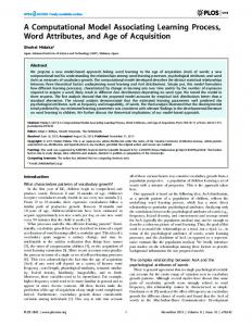
an exponential number of entities without the need to represent these explicitly. Based on the ..... Similarly, there exist plain angular head velocity cells (AHV cells) that ..... In order to determine the range of grid spacings and field sizes present in the ...... Figure 6.9: Eye and orbit anatomy with motor nerves by Patrick J. Lynch,.
A Computational Model of Grid Cells based on a Recursive Growing Neural Gas
Jochen Kerdels 2016
Research Report 1/2016
ISSN 1865-3944
© 2016 Jochen Kerdels
Editor: Type and Print: Distribution:
Dean of the Department of Mathematics and Computer Science FernUniversität in Hagen http://deposit.fernuni-hagen.de/view/departments/miresearchreports.html
A Computational Model of Grid Cells based on a Recursive Growing Neural Gas
Dissertation zur Erlangung des Grades eines
Doktors der Naturwissenschaften (Dr. rer. nat.) der Fakult¨at Mathematik und Informatik der FernUniversit¨at in Hagen vorgelegt von
Dipl.-Inform. Jochen Kerdels geb. in Nettetal Hagen, 16. September 2015
Gutachterin und Gutachter: Univ.-Prof. Dr. Gabriele Peters Univ.-Prof. Dr. Laurenz Wiskott
Acknowledgements I would like to thank my advisor Prof. Dr. Gabriele Peters who supported me and my research by providing continuous encouragement, subtle but decisive guidance and criticism, as well as the increasingly rare freedom to pursue basic research. The work at her group for Human-Computer Interaction at the University of Hagen is characterized by an open-minded, relaxed, and oftentimes cheerful atmosphere for which I would like to thank also my current and former colleagues Jens Garstka, Christoph Doppelbauer, and Dr. Klaus H¨ aming. I am especially grateful to Prof. Dr. Laurenz Wiskott and Prof. Dr. Sen Cheng from the University of Bochum who invited me to their monthly Hippocampus Club meetings. The friendly atmosphere, interesting discussions, and the constructive criticism I experienced in these meetings contributed significantly to this work. Furthermore, I would like to thank my dear friends Mathias H¨ ulsbusch, Prof. Dr. Jan Albiez, Thomas Kindler, Christiane R¨ utten, and Priska Herger for their continuous support and willingness to explore new ideas without prejudices regarding their validity or even sanity. Lastly, I would like to thank my parents. Their lifelong and unconditonal support is the foundation that allowed me to pursue my research in the first place.
3
4
Contents Preface
9
1 Spatial Representation in the Brain 1.1
11
The Parahippocampal-Hippocampal Region . . . . . . . . . . . .
11
1.1.1
Standard View of the PHR-HF Network . . . . . . . . . .
13
1.2
Place Cells . . . . . . . . . . . . . . . . . . . . . . . . . . . . . .
16
1.3
Head-Direction Cells . . . . . . . . . . . . . . . . . . . . . . . . .
18
1.4
Grid Cells . . . . . . . . . . . . . . . . . . . . . . . . . . . . . . .
19
1.5
Further Cell Types . . . . . . . . . . . . . . . . . . . . . . . . . .
21
1.5.1
Border Cells . . . . . . . . . . . . . . . . . . . . . . . . . .
21
1.5.2
Boundary Vector Cells . . . . . . . . . . . . . . . . . . . .
22
1.5.3
DG granule cells . . . . . . . . . . . . . . . . . . . . . . .
24
1.5.4
Spatial Representation in the Primate Brain
25
. . . . . . .
2 Grid Cell Properties
29
2.1
Grid Measures . . . . . . . . . . . . . . . . . . . . . . . . . . . .
29
2.2
Topographical Organization . . . . . . . . . . . . . . . . . . . . .
32
2.3
Realignment . . . . . . . . . . . . . . . . . . . . . . . . . . . . . .
33
2.4
Rescaling . . . . . . . . . . . . . . . . . . . . . . . . . . . . . . .
35
2.5
Fragmentation . . . . . . . . . . . . . . . . . . . . . . . . . . . .
37
2.6
Development . . . . . . . . . . . . . . . . . . . . . . . . . . . . .
39
2.7
Phase Precession . . . . . . . . . . . . . . . . . . . . . . . . . . .
40
2.8
Grid Cell Identification . . . . . . . . . . . . . . . . . . . . . . . .
41
2.9
Neuronal Structure . . . . . . . . . . . . . . . . . . . . . . . . . .
43
2.9.1
Neuron Morphology in the Entorhinal Cortex . . . . . . .
43
2.9.2
Neuron Morphology in the Pre- and Parasubiculum . . .
51
5
6
CONTENTS
3 Computational Models of Grid Cells 3.1
53
Oscillatory Interference Models . . . . . . . . . . . . . . . . . . .
54
3.1.1
Dendritic Oscillator Model . . . . . . . . . . . . . . . . .
55
3.1.2
Persistent Spiking Model . . . . . . . . . . . . . . . . . .
58
3.1.3
Ring Attractor Model . . . . . . . . . . . . . . . . . . . .
59
3.1.4
Coupled Neuron Models . . . . . . . . . . . . . . . . . . .
61
Continuous Attractor Network Models . . . . . . . . . . . . . . .
63
3.2.1
Dynamic Connection Model . . . . . . . . . . . . . . . . .
65
3.2.2
Fixed Connection Models . . . . . . . . . . . . . . . . . .
66
Hybrid OI/CAN Models . . . . . . . . . . . . . . . . . . . . . . .
69
3.3.1
Standing Wave Model . . . . . . . . . . . . . . . . . . . .
70
3.3.2
VCO-driven Attractor Model . . . . . . . . . . . . . . . .
71
Models Based On Self-Organization . . . . . . . . . . . . . . . . .
72
3.4.1
Long-distance Path Integration Model . . . . . . . . . . .
72
3.4.2
Neuronal Fatigue Models . . . . . . . . . . . . . . . . . .
73
3.4.3
Stripe Cell Models . . . . . . . . . . . . . . . . . . . . . .
74
3.5
Spatial Interference Model . . . . . . . . . . . . . . . . . . . . . .
76
3.6
Summary . . . . . . . . . . . . . . . . . . . . . . . . . . . . . . .
77
3.2
3.3
3.4
4 Computational Model 4.1
4.2
4.3
79
Model Intuition . . . . . . . . . . . . . . . . . . . . . . . . . . . .
79
4.1.1
GNG revisited . . . . . . . . . . . . . . . . . . . . . . . .
81
4.1.2
Basic Grid Cell Model . . . . . . . . . . . . . . . . . . . .
83
Model Definition . . . . . . . . . . . . . . . . . . . . . . . . . . .
86
4.2.1
Aspects of Recursion . . . . . . . . . . . . . . . . . . . . .
91
Biological Plausibility . . . . . . . . . . . . . . . . . . . . . . . .
92
5 Model Characterization
97
5.1
General Parameter Assessment . . . . . . . . . . . . . . . . . . .
97
5.2
Modeling Grid Cells . . . . . . . . . . . . . . . . . . . . . . . . .
99
5.2.1
Fixed Parameters . . . . . . . . . . . . . . . . . . . . . . .
99
5.2.2
Variable Parameters . . . . . . . . . . . . . . . . . . . . . 100
5.2.3
Grid Cell Measures . . . . . . . . . . . . . . . . . . . . . . 101
5.3
Baseline Experiments
. . . . . . . . . . . . . . . . . . . . . . . . 104
CONTENTS
7
5.3.1
Isolated Bottom Layer . . . . . . . . . . . . . . . . . . . . 104
5.3.2
Isolated Top Layer . . . . . . . . . . . . . . . . . . . . . . 112
5.3.3
Coupled Top and Bottom Layer
5.4
. . . . . . . . . . . . . . 134
Discussion . . . . . . . . . . . . . . . . . . . . . . . . . . . . . . . 155
6 Input Space Aspects
167
6.1
Sequential Input . . . . . . . . . . . . . . . . . . . . . . . . . . . 167
6.2
Noisy Input . . . . . . . . . . . . . . . . . . . . . . . . . . . . . . 171
6.3
Input Space Instances . . . . . . . . . . . . . . . . . . . . . . . . 172
6.4
6.3.1
1D Attractor Network Input
. . . . . . . . . . . . . . . . 173
6.3.2
Place Cell Input . . . . . . . . . . . . . . . . . . . . . . . 175
6.3.3
Eye Gaze Input . . . . . . . . . . . . . . . . . . . . . . . . 177
Discussion . . . . . . . . . . . . . . . . . . . . . . . . . . . . . . . 181
7 Outlook
183
7.1
Encoding . . . . . . . . . . . . . . . . . . . . . . . . . . . . . . . 183
7.2
Hierarchical Organization . . . . . . . . . . . . . . . . . . . . . . 187
7.3
Summary and Conclusion . . . . . . . . . . . . . . . . . . . . . . 190
A Appendix
193
A.1 Supplementary Empirical Data . . . . . . . . . . . . . . . . . . . 193 A.2 Supplementary Simulation Data . . . . . . . . . . . . . . . . . . . 195 A.3 Supplementary Implementation Details . . . . . . . . . . . . . . . 198 Bibliography
199
8
CONTENTS
Preface In 1948 Edward Tolman [164] reported on a series of behavioral experiments with rats that led him to hypothesize that the animals had to make use of an internal, map-like representation of the environment. This idea, which came to be known as the cognitive map hypothesis, was highly controversial at the time. Accordingly, the discovery of hippocampal place cells by O’Keefe and Dostrovsky [119, 121] in the 1970s was met with much excitement as place cells were the first possible direct evidence for such a representation of the environment in the brain [120]. Since then a variety of neurons that exhibit spatially correlated activity were found in the parahippocampal-hippocampal region [163, 79, 45, 62, 152]. In particular the recent discovery of grid cells [45, 62] in the entorhinal cortex of rat strengthened the idea that the involved neuronal structures constitute a kind of metric for space [112]. Grid cells are neurons that exhibit spatially correlated activity possessing multiple, discrete firing fields that are arranged in a regular, hexagonal grid that spans the entire environment. Located just one synapse upstream of the hippocampus grid cells are assumed to be an important source of spatial information to place cells [153, 135]. In particular, grid cells are generally considered to be a central part of a path integration system as pointed out by Burgess [19]: There has been a surprising rapid and general agreement that the computational problem to which grid cells provide a solution is “path integration” within an allocentric reference frame. Although existing computational models cover a wide range of possible mechanisms and focus on different aspects of grid cell activity [112, 170, 55, 2, 13, 114], the models share the common approach of explaining grid cells and their behavior as functional components within the cognitive map hypothesis. Complementary to this common approach this thesis presents an alternative grid cell model that treats the observed grid cell behavior as an instance of a more abstract, general principle by which neurons in the higher-order parts of the cortex process information. The first two chapters provide a brief neurobiological background on grid cells. Chapter 1 introduces their “cortical neighborhood”. It describes the parahippocampal-hippocampal region and its major internal connectivity. Furthermore, it summarizes the findings on neurons from this region that, like grid cells, exhibit a spatially correlated firing behavior. Chapter 2 focuses then on the particular properties of grid cells and introduces the basic measures 9
10
CONTENTS
that are used throughout the literature to characterize them: grid spacing, grid orientation, grid field size, grid phase, and most importantly the gridness score. In addition to findings on specific properties of the grid cell firing behavior, the chapter also provides information on the possible neural substrate of grid cells. This information is used later in chapter 5 to derive a biologically plausible parametrization of the grid cell model. Following this introduction of grid cells and their properties the third chapter presents an extensive overview on existing computational models of grid cells. The overview is structured by the commonly used classification of grid cell models into either oscillatory interference models, continuous attractor network models, or models based on mechanisms of self-organization. The chapter illustrates that, despite the diversity in the proposed mechanisms, essentially all existing computational models are grounded in the cognitive map hypothesis assuming that grid cells are a specialized, functional part of a system that supports navigation and self-localization. The next three chapters constitute the main part of this thesis. Chapter 4 introduces and defines a novel grid cell model that is not grounded in the cognitive map hypothesis. Instead, it is based on the core assumption that the behavior of grid cells is just one instance of a general processing scheme in which the specific behavior of a group of neurons is defined by two factors: the general characteristics of this common processing scheme and the specific properties of the particular input space. In chapter 4 this putative general processing scheme is formally defined by a novel algorithm called the recursive growing neural gas (RGNG), which extends the original growing neural gas algorithm introduced by Bernd Fritzke in 1995 [41]. The RGNG algorithm describes the behavior of a whole group of cells that can replicate the behavior of a grid cell group given an input space with suitable properties. In chapter 5 the RGNG model is extensively tested and characterized with respect to a wide range of key parameters. As its main result the chapter demonstrates that the RGNG is indeed able to replicate the core properties of grid cell behavior based on a minimal set of assumptions regarding the properties of the used input space. Having established the viability of the RGNG model chapter 6 focuses on the influence of changes to the input space on the resulting RGNG behavior. It shows that the RGNG can handle sequential input that reveals the input space structure only over a longer timescale and it demonstrates the robustness of the RGNG model towards noisy inputs. Furthermore, the chapter investigates two alternative input spaces that illustrate the broad applicability of the RGNG model with respect to other types of input. Finally, chapter 7 outlines the broader implications of the presented general processing scheme. It highlights the exponential encoding capacity of the RGNG model and provides a basic mechanism that shows how this capacity can be utilized in a hierarchical, autoassociative memory that has the ability to store an exponential number of entities without the need to represent these explicitly. Based on the ideas presented in this last chapter it is likely that the RGNG-model may find uses outside of its main neuroscientific objective, e.g., as a potential object of research in the area of machine learning.
Spatial Representation in the Brain Beginning with the discovery of place cells in the CA1 area of the hippocampus by O’Keefe and Dostrovsky [119, 121] in the 1970s, increasing evidence [163, 79, 45, 62, 152] indicates that the parahippocampal-hippocampal region of the brain is vital to the representation of spatial, allocentric information in the brain. In particular the recent discovery of grid cells in the entorhinal cortex by the Moser group [45, 62] and their subsequent investigation led to the hypothesis that the involved neuronal structures constitute a kind of metric for space [112, 111]. This chapter provides an overview of the structures found in the parahippocampalhippocampal region of the brain and summarizes the types of neurons that were found to exhibit spatially correlated activity. If not stated otherwise the neuronal structures reported here refer to the rat brain.
1.1
The Parahippocampal-Hippocampal Region
The parahippocampal-hippocampal region consists of the parahippocampal region (PHR) and the hippocampal formation (HF). Figure 1.1 shows the position of all areas that comprise this region and provides details on their layered cortical structure. The PHR is subdivided into five main areas: the perirhinal cortex (PER; consisting of Brodmann areas A35 and A36), the postrhinal cortex (POR), the presubiculum (PrS), the parasubiculum (PaS), and the entorhinal cortex (EC; consisting of a lateral (LEA) and medial (MEA) part). The areas of the PHR have a layered structure and exhibit, similar to the neocortex [155], six distinct layers which are typically denoted with the roman numerals I to VI. Layers II/III and layers V/VI are principal cell layers containing the soma of different types of pyramidal neurons as well as interneurons. Layers I and IV are plexiform layers that contain dendrites of principal cells and interneurons. Layer IV, which separates the principal cell layers is also referred to as lamina dissecans [175, 154, 166, 160]. In case of PER and POR layer IV is “variably developed” [166], i.e., the layer is not always clearly identifiable between layer III and layer V. Rapp et al. [131] provide an estimate of the number of neurons in the PHR of rat based on measurements in six animals. Per hemisphere, the perirhinal cortex 11
12
CHAPTER 1. SPATIAL REPRESENTATION IN THE BRAIN
Figure 1.1: Overview of the parahippocampal-hippocampal region in the rat brain. (A) Schematic views (lateral and caudal) on the PHR and HF within the rat brain. (B) Nissl-stained slices through the PHR and HF with color-coded and labeled subfields. (C) Enlarged version of the horizontal cross-section Bb with labeled cortical layers of most PHR and HF subareas (POR not visible). Reproduced from van Strien et al. [166]. contains about 2.8 × 10⁵ neurons, the postrhinal cortex contains about 1.1 × 10⁵ neurons, the medial entorhinal cortex contains about 2.6 × 10⁵ neurons, and the lateral entorhinal cortex contains about 3.7 × 10⁵ neurons. The HF is subdivided into four main areas: the dentate gyrus (DG), the cornu ammonis 3 (CA3), the cornu ammonis 1 (CA1), and the subiculum (Sub). The border region between CA3 and CA1 is referred to as cornu ammonis 2 (CA2). As CA2 is small and under-investigated in the rat it is often not discussed in depth in the literature [166]. The hilus (see below) of DG is sometimes referred to as cornu ammonis 4 (CA4) when it is treated as a part of the hippocampus rather then the dentate gyrus. The areas of the HF have a three-layered structure. They have a deep, polymorphic layer containing afferent and efferent fibers as well as a variety of interneurons, a central layer containing the soma of principal neurons and interneurons, and a superficial layer containing afferent fibers and dendrites of principal neurons [175, 154, 166, 160].
1.1. THE PARAHIPPOCAMPAL-HIPPOCAMPAL REGION
13
In the DG the deepest layer is called the hilus or stratum multiforme. Among other types of neurons this layer contains mossy cells which project their characteristic, unmyelinated axons to CA3. The principle cell layer of DG is called the granular layer (stratum granulare) and contains the somas of granule cells. The dendrites of these cells extend into the superficial layer, called the molecular layer (stratum moleculare). Depending on the afferent fibers that contact the dendrites the molecular layer is further subdivided into inner, middle, and outer molecular layer [166, 160]. In the CA areas the principle cell layer (stratum pyramidale) is dominated by the soma of pyramidal neurons. Below this layer lies stratum oriens which contains the basal dendrites of the pyramidal cells. Above the principal cell layer lies the molecular layer which is subdivided into stratum lucidum, stratum radiatum, and stratum lacunosum moleculare. Stratum lucidum receives input from DG and is missing in CA2 and CA1. Stratum radiatum contains the apical dendrites of the pyramidal cells and stratum lacunosum moleculare contains the apical tufts of those apical dendrites [166, 160]. The Subiculum has a very broad principle cell layer containing large soma of pyramidal neurons and a variety of smaller interneurons. The polymorphic layer below the principle layer is very thin and therefore usually neglected. The molecular layer above the principle cell layer is subdivided into deep and superficial sublayers. The deep sublayer aligns with the stratum radiatum of CA1, whereas the superficial sublayer corresponds to the stratum lacunosum moleculare [166, 160]. West et al. [171] provide an estimate of the number of neurons in the HF of rat based on measurements in five animals. Per hemisphere, the granular layer of the DG contains on average 1.2 × 10⁶ neurons, the hilus contains about 5.3 × 10⁴ neurons, the principle layer of CA3 contains about 2.5 × 10⁵ neurons, the principle layer of CA1 contains about 3.8 × 10⁵ neurons, and the subiculum contains about 2.8 × 10⁵ neurons.
1.1.1
Standard View of the PHR-HF Network
According to a recent review of van Strien et al. [166] the various circuitry models of the PHR-HF network that can be found in current literature can be aggregated into a standard view of the PHR-HF network. This standard view is depicted in figure 1.2. It shows that neocortical input to the HF as well as hippocampal output to the neocortex is mediated by the PHR. Within the PHR two main projection streams are distinguished. The PER is considered to provide the main input to the LEA, whereas the POR provides the main input to the MEA. In both cases backprojections from LEA to PER and MEA to POR exist. In addition, the PrS provides input to the EC as well. Originating from the EC the perforant pathway projects to all subareas of the HF. The perforant pathway consists of axons from EC layer II neurons projecting to the DG and CA3 as well as axons from EC layer III neurons projecting to CA1 and the subiculum. Within the HF the subregions are connected sequentially from the DG via CA3 and CA1 to the subiculum. Finally, output of the HF projects from CA1 and the subiculum back to the deep layers V and VI of the EC.
14
CHAPTER 1. SPATIAL REPRESENTATION IN THE BRAIN
Figure 1.2: The standard view of the parahippocampal-hippocampal network based on the review by van Strien et al. [166]. In contrast to this standard view the connections between different areas of the PHR-HF region are much more intricate. Based on data compiled by van Strien et al. [166] figure 1.3 depicts the PHR-HF network as an adjacency matrix. This more detailed view shows that the perirhinal cortex (PER) projects also to the MEA and that the postrhinal cortex (POR) projects also to the LEA. In addition, the input to the HF is not restricted to originate only from the EC. All subareas of the HF receive projections from the presubiculum (PrS), the parasubiculum (PaS), the perirhinal (PER) and postrhinal (POR) cortices. Furthermore, the detailed view shows that the seemingly sequential connection of areas in HF is more complicated. CA3 and CA1 have backprojections to the DG; CA1 has backprojections to CA3; and CA3 has projections to the subiculum. The output of the HF is more diverse as well. CA1 and the subiculum have projections to the presubiculum (PrS) and parasubiculum (PaS); CA1 has projections to the postrhinal cortex (POR); and all subareas of the HF have projections to the perirhinal cortex (PER). The adjacency matrix in figure 1.3 provides also some insight into intra-area networks. For example, in the HF the principle cells of areas CA3, CA1, and the subiculum all project into other layers of the particular regions. However, in the dentate gyrus (DG) this is not the case. In the DG the cells of the hilus and not the principle granule cells are those that project within the area. This raises the interesting question where the numerous granule cells of the DG actually project to. Based on the data compiled by van Strien et al. [166] possible targets are only the stratum lucidum of CA3 or the perirhinal cortex (PER). Comparing the HF with the PHR the increase in intra-area connectivity of the particular regions is striking. Especially the entorhinal cortex (EC) and the presubiculum (PrS) stand out in this regard. The latter receiving substantial input from CA1 and the subiculum across all layers and thus, as the presubiculum also acts as input to the entorhinal cortex, establishing an additional, indirect feedback path from the HF to the EC.
POR
A36
A35
LEA
MEA
PaS
PrS
Sub
CA1
CA3
DG
to oml mml iml gra hilus slm rad luc pyr or slm rad pyr or ml-sup ml ml-deep pyr I II III IV V VI I II III IV V VI I II III IV V VI I II III IV V VI I II III IV V VI I II III IV V VI I II III IV V VI
from
oml
oml
mml
mml
rad pyr CA1
or
1 1 1
ml-sup
1 1
1 1
ml-deep
1 1
1 1
Sub
1 1 1 1 1
1 1
1 1 pyr
1 1 ml
1 1
1 1
1 1 1 1 1 1 1
1
1 1 1 1
pyr
known source and destination layer
slm
1 1 1
1 1 1
ml-deep
Sub
1 1
1 1 1 1 1 1
ml
unknown source or destination layer
or
1 1 1
1 1 1 1 1 1
1 1
ml-sup
standard model projections within HF
pyr
1
1
1 1 1
1
1 1 1 1 1
1
1
1
1
1
1
or
standard model PHR to HF projections
hilus
1
1
1
1
1
CA1 rad pyr
1 1 1 1
slm 1
or
1
pyr
1
luc CA3
CA3 luc
1 1
rad
rad
1
slm
slm
1
1
hilus 1 1 1 1 1
unknown source and/or destination layer
gra
gra
standard model projections within PHR
iml DG
DG iml
I
1 1 1
1
1
1
1
I
II
1 1 1
1 1 1 1 1
1 1 1 1 1 1
1
1
II
IV
V
1 1 1
1 1 1
1 1 1 1 1
1
1 1 1 1 1 1 1
1
1
V
VI
1 1 1
1 1 1 1 1
1 1
1 1
1
1
VI
I
1
1
1
I
known source and destination layer
unknown source and/or destination layer
III
1 1 1
1 1 1
1
1
1
1
IV
1
PrS
PrS
1
1
1 1
1
1
1
III
II
1
1
1
1
1
1
1
II
III
1 1
1 1
1
1
1
1
1
1
III
PaS
PaS
IV
1
1
1
IV
V
1
1
1
1
1
1
1
V
VI
1
1
1
VI
I
1 1
1
1
I 1 1
II
1 1 1 1 1
1 1 1
1 1
1 1
1
1 1
1 1
II 1 1
III
1 1 1 1 1
1 1 1
1 1 1
1 1 1
1
1 1
1 1
III 1 1
MEA
MEA
IV
1 1 1 1 1 1
1 1 1 1
1 1 1
1
IV
V
1 1 1 1
1 1 1
1 1
1 1 1
V
VI
1 1 1 1 1 1 1 1 1 1 1 1 1 1 1 1 1 1 1 1 1
VI 1 1 1 1 1
I
I
II
1 1 1
1 1 1
1
1
1
1
1
1
II 1
III
1 1 1 1 1 1 1 1 1 1 1 1 1 1 1 1 1 1 1 1 1 1 1 1 1 1
1 1 1
1
1 1 1
1
1
III 1
LEA
LEA
IV
1
1 1 1
1 1 1 1 1 1
1 1
1
1
1
1
IV 1
V
1 1 1 1 1 1 1 1 1 1 1 1 1 1 1 1 1 1
1 1 1
1
1
V 1
VI
1
1 1 1 1 1 1 1 1 1 1 1 1
1 1 1
1
1
1
1
VI 1
I
I
II
1
1 1 1 1 1 1 1 1
1 1
II
III
1 1 1 1 1 1
1 1
III
A35
A35
IV
IV
V
1 1
V
VI
1
1 1
1 1
VI
PER
PER
I
I
II
1
1 1 1 1 1 1 1
1 1
1 1
II
III
1 1 1 1 1 1
III
A36
A36
IV
IV
V
1
1 1 1 1 1 1 1
1 1
1 1
V
VI
1
1 1 1 1 1 1 1
1 1
1 1
VI
I
I
II
1 1
1 1 1 1 1 1 1 1 1 1 1 1 1
1 1 1
II
III
1 1 1
III
POR
POR
IV
IV
V
1 1
1 1 1 1 1 1 1 1 1 1 1 1 1
1 1 1
V
VI
1 1
1
VI oml mml iml gra hilus slm rad luc pyr or slm rad pyr or ml-sup ml ml-deep pyr I II III IV V VI I II III IV V VI I II III IV V VI I II III IV V VI I II III IV V VI I II III IV V VI I II III IV V VI
POR
A36
A35
LEA
MEA
PaS
PrS
Sub
CA1
CA3
DG
1.1. THE PARAHIPPOCAMPAL-HIPPOCAMPAL REGION 15
Figure 1.3: Adjacency matrix of the parahippocampal-hippocampal network based on data compiled by van Strien et al. [166]. Columns and rows representing areas of the hippocampal formation (HF) are marked green. Columns and rows representing areas of the parahippocampal region (PHR) are marked red. Blue colored cells containing a “1” represent connections with known source and destination layers. Olive shaded cells represent connections with unknown source and/or destination layers. Violet shades represent connections within an area. Cells that represent connections which constitute the standard view of the parahippocampal-hippocampal network are tinted green within HF, tinted red within PHR, and are tinted yellow if they connect PHR with HF or vice versa.
16
CHAPTER 1. SPATIAL REPRESENTATION IN THE BRAIN
(a)
(b)
Figure 1.4: Examples of activity in a single place cell (a) and a single grid cell (b). Black lines represent the trajectory of a rat in a square environment. Red dots represent the locations where the observed place cell or grid cell fired. Figure from Moser et al. [111].
External input to the parahippocampal-hippocampal region from unimodal and polymodal associational areas is received predominantly by the perirhinal and postrhinal cortices. The perirhinal cortex receives about 48% olfactory, 19.5% auditory, 12% somatosensory, 10% visuospatial, 7.5% visual, and 3% gustatory inputs. Area 35 of the perirhinal cortex receives almost exclusively the olfactory inputs whereas all other inputs are received primarily in area 36. The postrhinal cortex receives about 62% visual, 30% visuospatial, 5% auditory, 2% somatosensory, and 1% gustatory inputs. Although to a lesser extent the entorhinal cortex itself receives some external inputs from associational areas. For the LEA the distribution of input modalities is similar to that of the perirhinal cortex. In case of the MEA the distribution of input modalities is similar to that of the postrhinal cortex [24]. It should be noted that the preceding description of the PHR and the HF is to some degree an oversimplification. It only outlines the coarse structure and circuitry of the particular areas. Detailed examinations of, e.g., anatomical structures, existing neuron types, or biochemical properties exist for many areas in the PHR-HF region, e.g., for the entorhinal cortex [92, 68, 110, 17].
1.2
Place Cells
In the 1970s O’Keefe and Dostrovsky were the first to discover neurons in the CA1 region of the hippocampus that exhibit spatially correlated activity [119, 121]. They termed these neurons place cells as their firing pattern correlated strongly with specific places – the cells’ place fields – in the environment. Figure 1.4a shows such a place field of a single neuron. The majority of place cells O’Keefe and Dostrovsky found were “plain” place cells with single place fields1 of sizes ranging from 10cm2 to half the recording environment2 and a firing pattern 1A
few place cells had two or more place fields. circular platform with a diameter of 35cm and three radiating arms of 38cm in length and 15cm in width [121]. 2A
1.2. PLACE CELLS
17
correlated solely to the rat’s allocentric position. Besides these “plain” place cells, the activity of some cells appeared to be modulated by additional factors like the current behavior, e.g., sniffing or eating, and the rat’s orientation. The activity of place cells appears to be determined by external cues, e.g., distant visual cues as well as internal cues, e.g., information about locomotion [121]. For example, if a rat is placed on a platform surrounded by curtains that provide a stable, visual environment a rotation of the platform does not cause a rotation of the place fields’ locations. They appear fixed with respect to the visual cues provided by the curtains. As expected, the place fields do rotate if the surrounding curtains are rotated instead of the platform. However, if the lights are switched off and the rat moves in the dark, the position of the rat as indicated by the activity of corresponding place cells is updated nevertheless, i.e., the activity of place cells is not exclusively determined by external cues but relies also on internal cues about the animal’s locomotion. Further investigation of the influence of distant visual cues on place cell activity revealed the phenomenon of remapping [118, 115]. For a given environment a certain set of place cells represents this particular environment. When the environment changes, e.g., when a rat is placed from one experimental environment into another, a different set of place cells gets recruited to represent the new environment. This switch from one set of place cells to another is termed global remapping [97, 75] and it only occurs if the environment changes significantly. If, in contrast, the environment changes only slightly, the same set of place cells is used but the maximum intensity with which individual place cells are active changes. This change of maximum activity is termed rate remapping [97]. The discovery of place cells raised much excitement as these cells were the first possible evidence on the neuronal level for the cognitive map hypothesis stated by Tolman back in 1948 [164]. Based on the observations made in a series of behavioral experiments with rats Tolman concluded that the observed behavior would require a map-like, allocentric representation of the environment in the rat’s brain. Some of the observed, prominent features of place cells support this hypothesis. As such, many researchers interpret the results of place cell experiments from the perspective of this hypothesis [120]. However, more recent work on place cells challenges this view. For example, Eichenbaum et al. [34] point out that “non-plain” place cells, i.e., place cells that are modulated by behavior, or more generally by context, may be underrepresented in most experiments. They argue that the typical setup of most place cell experiments3 results in an unusual high proportion of detected “plain” place cells. In contrast, if the experiment contains a behaviorally more demanding task and a richer environment, the proportion of “plain” place cells is typically much lower. Eichenbaum et al. suggest that place cell is possibly a misnomer and that place cells are more likely to be cells that generally identify significant combinations of high-level, multimodal signals. From that perspective, the cells in the hippocampus are more likely to encode a form of episodic, contextual memory instead of a predominantly spatial map. This view is supported by findings in the human hippocampus 3 The typical setup of a place cell experiment consists of a single rat within a small (0.5 to 1m2 ) circular or rectangular environment performing the random foraging task, i.e., the rat searches for food pellets thrown randomly in the environment.
18
CHAPTER 1. SPATIAL REPRESENTATION IN THE BRAIN
where especially the left hippocampus is primarily involved in storing linguistic relationships and narratives rather than spatial relationships [22]. Another indication that the interpretation of experimental results regarding place cells may have been biased by the experimental setup that is commonly used is given by Fenton et al. [37]. They measured and compared the activity of CA1 place cells in a standard cylinder environment and in a chamber environment approximately six times larger. The cylinder environment was placed in the chamber environment to allow for a transition between the two environments by simply removing the wall of the cylinder environment. Within the standard cylinder the cells’ activity patterns corresponded to typical place cell activity as it is reported in the literature, i.e., the majority of place cells had a single place field. In contrast, within the larger chamber environment the majority of place cells had multiple, irregularly spaced, and enlarged place fields. In addition, the switch between the two environments caused a global remapping of those place cells that were active in both environments. These results show that individual place cells do not primarily encode single spatial locations but rather use some form of ensemble encoding to disambiguate among the multiple spatial locations represented by individual cells. This new perspective on place cells suggests that the spatial information contained in the place cell signal may not originate in the hippocampus but is generated somewhere upstream [98]. A good candidate region in this regard is the entorhinal cortex with its population of grid cells which are described in detail in section 1.4.
1.3
Head-Direction Cells
A different form of spatial signal is encoded by so-called head-direction cells (HD cells) first described by Taube et al. in 1990 [163]. In contrast to place cells the firing pattern of HD cells correlates with the allocentric head direction of the animal, i.e., the peak firing rate of a HD cell is reached when the animal’s head points in the preferred spatial direction of that cell. Centered around this preferred direction is the cell’s directional firing range in which the firing rate is above the cell’s baseline firing rate. Firing ranges can vary between 60◦ and 150◦ . For most cells the average directional firing range is about 90◦ [161]. The preferred spatial direction of HD cells is influenced by external cues in a way similar to that of place cells. If a prominent visual cue in a circular environment is rotated, the preferred spatial directions of HD cells shift correspondingly [162]. In addition, if a novel prominent visual cue is introduced it gradually takes control of the cell’s preferred spatial direction within minutes, i.e., rotation of the novel cue leads to a corresponding rotation of the cell’s preferred spatial directions. In contrast, the removal of visual cues, e.g., by turning the lights off, affects the firing behavior of HD cells just minimally in that the preferred spatial direction of the cells may drift by an unpredictable amount after some time [57]. While running in the dark, the firing behavior of the animal’s HD cells can be maintained by idothetic information like proprioceptive or vestibular signals alone. In addition to their directional tuning some HD cells are also modulated by the animal’s angular head velocity, i.e., their peak firing rate increases proportional
1.4. GRID CELLS
19
Figure 1.5: Typical visualization of a grid cell’s firing pattern as introduced by Hafting et al. [62]. Left: trajectory (black lines) of a rat in a circular environment with marked locations (red dots) where the observed grid cell fired. Middle: color-coded firing rate map of a single grid cell ranging from dark blue (no activity) to red (maximum activity). Right: color-coded spatial autocorrelation of the firing rate map ranging from blue (negative correlation, -1) to red (positive correlation, +1). Figure from Moser et al. [112]. to the velocity with which the animal is turning its head across the cell’s preferred spatial direction. Similarly, there exist plain angular head velocity cells (AHV cells) that encode just the angular head velocity independent of the absolute head direction. AHV cells can be further divided into symmetric and asymmetric AHV cells. Symmetric AHV cells fire proportional to the angular head velocity irrespective of the turning direction whereas asymmetric AHV cells fire only when the head turns either clockwise or counter-clockwise [161]. HD cells can be found in a variety of areas in the brain including the parahippocampal region (pre- and parasubiculum, entorhinal cortex), the retrosplenial cortex neighboring the PHR and several thalamic nuclei. AHV cells are predominantly found in areas of the brainstem like dorsal tegmental nucleus, nucleus prepositus, or medial vestibular nucleus [161, 9].
1.4
Grid Cells
The notion that place cells in the hippocampus may rather represent contextspecific information than mainly location-specific information suggests that context-independent position information could be computed by cells in areas preceding the hippocampus. The recent discovery of grid cells by Fyhn et al. supports this hypothesis [45, 62, 112, 111]. Grid cells are neurons that exhibit spatially correlated activity similar to that of place cells with the distinct difference that grid cells possess not just one but multiple, discrete firing fields that are arranged in a regular, hexagonal grid that spans the entire environment. Examples for this peculiar firing pattern of grid cells are given in figures 1.4b and 1.5, which show the firing fields of a single grid cell. In order to characterize grid cells based upon their particular firing patterns Hafting et al. [62] introduced four measures to describe the spatial properties of the grid structure: spacing, orientation, field size, and phase. Three of these measures (spacing, orientation, and field size) are calculated using the
20
CHAPTER 1. SPATIAL REPRESENTATION IN THE BRAIN
autocorrelogram of the grid cell’s firing rate map (fig. 1.5)4 . The spacing of a grid cell is defined as the median distance between the central peak of the autocorrelogram and its six surrounding peaks. The orientation of a grid cell is defined as the angle between a fixed reference line (0 degrees) going through the central peak of the autocorrelogram and a vector from the central peak to the surrounding peak on the right side that is nearest to the reference line in counterclockwise direction. The field size of a grid cell refers to the size of the individual firing fields. It is estimated as the area occupied by the central peak in the autocorrelogram. The phase of a grid cell refers to the position of the cell’s firing fields, i.e., their grid vertices, with respect to the firing fields of other cells with similar spacing and orientation. If the rate maps of two grid cells are cross-correlated, the resulting cross-correlogram resembles the autocorrelogram of a single grid cell but the central peak will be off center. The distance from the center to this displaced central peak is defined as the phase difference between the two grid cells. These four measures are widely adopted and used throughout the grid cell literature. In addition to these measures Sargolini et al. introduced a gridness score which allows to quantify how well an observed cell qualifies as being a grid cell [141]. The gridness score is based on the autocorrelogram of the cell’s firing rate map. To calculate the score only the six peaks surrounding the central peak in the autocorrelogram are taken into account. All other regions of the autocorrelogram including the central peak are masked out. Then, the correlation values between the masked autocorrelogram and rotated versions of itself at 30◦ , 60◦ , 90◦ , 120◦ , and 150◦ are computed. Finally, the gridness score is defined as the difference between the lowest correlation value at 60◦ and 120◦ and the highest correlation value at 30◦ , 90◦ , and 150◦ . Typically, a cell is classified as grid cell if its gridness score is positive. Grid cells were found in the medial entorhinal cortex as well as recently in the pre- and parasubiculum [62, 141, 9]. In the MEA grid cells are most abundant in layers II and III. They make up about 50% of all neurons in layer II and about 40% of all neurons in layer III. In layers V and VI of the MEA grid cells are less frequent (about 20% to 25%). Grid cells in layers III, V, and VI of MEA are colocated with head direction cells and conjunctive grid × head direction cells5 . The latter are cells with a grid cell like firing pattern modulated by head direction. In the pre- and parasubiculum grid cells are uniformly distributed across all layers, albeit with a significantly lower proportion compared to the MEA (about 13% in PrS and 20% in PaS). Similar to the deep layers of MEA the grid cells in PrS and PaS are colocated with head direction and conjunctive cells [141, 9]. In the MEA grid cells are topographically organized. Neighboring grid cells share similar spacing, orientation, and field size, but have typically dissimilar phases. With distance from the postrhinal border spacing and field size of grid cells increase along the dorsoventral axis of the entorhinal cortex [62]. In a recent study Stensola et al. showed that this increase in spacing and field size is discretized [156]. They estimate that the MEA contains less than ten distinct 4 A detailed account how the firing rate map and the autocorrelogram are calculated is given in chapter 2. 5 Sometimes conjunctive grid × head direction cells are just referred to as conjunctive cells.
1.5. FURTHER CELL TYPES
21
clusters of grid cells or grid modules and that each cluster contains grid cells with specific spacing and field size. Moreover, Stensola et al. could also show that the cells in each grid module share a common orientation. Orientation and phase of grid cells is controlled by external cues. The phase of a grid cell in a given environment stays constant across successive exposures to this environment. This stability suggests, that the phase is anchored to some external cues of the environment rather than being based on idiothetic cues. In case of the grid cell’s orientation it can be shown, that the rotation of a prominent visual cue in a circular environment leads to a corresponding rotation of the grid cell’s orientation. Removal of external cues, e.g., by switching of the light, does not affect the firing patterns of grid cells indicating that the grid structure itself is not dependent on external cues [62]. Under conditions that would lead to a remapping of place cells, i.e., a complete or partial recruitment of a different set of place cells to represent the new environmental conditions, grid cells undergo a realignment: the same set of grid cells stays active but orientation and phase of the grid cells may change [44]. A detailed account of these and further grid cell properties is given in chapter 2.
1.5
Further Cell Types
In addition to the three kinds of spatial representations described above there are further, but less investigated neurons with spatially correlated activity. Among those cells are border cells in the medial entorhinal cortex [152, 142] and preand parasubiculum [9], boundary vector cells in the subiculum [99, 158], and cells with spatial selectivity in the dentate gyrus [79]. Furthermore, there are reports on cells with place-cell-like and grid cell like firing behavior in the primate hippocampus and entorhinal cortex, respectively [49, 83]. In contrast to the corresponding cells in the rat the cells in the primate do not encode the animals position but rather a position in the allocentric view of the environment.
1.5.1
Border Cells
Cells in the entorhinal cortex as well as the pre- and parasubiculum possess firing fields that appear to represent borders or barriers in the immediate environment of the animal [152, 142, 9]. Such border cells fire whenever the animal is close to a border of its environment that lies in a certain, allocentric direction, e.g., a cell may just be responsive to eastern borders of the environment. Border cells are typically colocated with grid cells and head direction cells and make up only a small percentage (< 10%) of the local cell population. They were found in all layers of MEA and PrS/PaS. 75% of the border cells observed in the MEA had firing fields along a single wall whereas the rest had firing fields at up to four walls [152]. Figure 1.6 illustrates the typical firing behavior of a single border cell within different environments (A vs. B/C) and under different environmental configurations. The activity of the border cell persists across various manipulations of the environment that would commonly trigger a remapping of place cells
22
CHAPTER 1. SPATIAL REPRESENTATION IN THE BRAIN
Figure 1.6: Firing rate maps of a single border cell in different environments (A vs. B/C) with changing environmental configurations. Dark blue color equals zero, red color equals peak firing rate, which is indicated above each panel. A: When a square environment is stretched into a rectangular environment the firing field of the border cell stays attached to “its” border. B: When a new border is introduced to the environment (middle panel) a corresponding new firing field of the border cell appears. C: When the walls surrounding an environment are removed (middle panel) – resulting in a drop at the platform edges of about 60cm – the firing field of the border cell is preserved. Figure adapted from Solstad et al. [152]. and a realignment of grid cells, respectively. If the environment is suddenly expanded (A) the firing field of the border cell sticks to the border corresponding to its preferred border direction. If a new border is introduced (B) a firing field instantaneously emerges along the new border. If the walls of an environment are removed (C) resulting in a platform environment with a 60cm drop along its edges, the activity of the border cell still persists. These properties of border cell activity suggest, that border cells encode proximal obstacles in the environment of the animal that lie in a certain, allocentric direction. This direction can be controlled by external cues similarly to place cells and grid cells. The rotation of a cue card in the environment leads to a corresponding rotation of the border cell’s firing field. During such an environmental change the relative border directions within a group of border cells are retained, e.g., two border cells with firing fields at opposite walls in one environment fire at opposite walls in a different environment [152, 142]. As border cells provide information about obstacles and borders of the environment it is hypothesized [152] that border cells may provide a reference frame for other forms of spatial representation like place cells and grid cells by anchoring the firing positions of those cells to the geometric properties of the particular environment.
1.5.2
Boundary Vector Cells
In 1996 O’Keefe and Burgess discovered that the geometry of place fields would change in response to transformations of the environment, e.g., if a square environment is transformed into a rectangular environment, the firing fields of
1.5. FURTHER CELL TYPES
23
Figure 1.7: Illustration of the boundary vector cell (BVC) model. A: A BVC has a receptive field which is located at a fixed, small distance relative to the animal’s position but always oriented in a fixed, allocentric direction. B: With increasing distance the receptive field of a BVC gets broader and the resulting firing rate map exhibits a stripe-like pattern parallel to the particular boundary. C: Example of a BVC firing rate map resulting from a receptive field with short distance and eastward direction. D: Resulting firing rate maps of the BVC from (C) in different environment configurations. Figure from Lever et al. [99]. place cells stretch correspondingly [122]. In order to explain this phenomenon they developed a computational model of place cells that predicted the existence of boundary vector cells (BVCs) to provide the necessary input to the place cells in their model [122, 21, 63]. According to this model the receptive field of a BVC is located at a fixed, small distance relative to the animal’s position but always oriented in a fixed, allocentric direction (fig. 1.7A). The BVC fires whenever its receptive field is intersected by a boundary of the environment. Figures 1.7C and 1.7D illustrate the resulting firing rate maps of a BVC for different environment geometries. In case the receptive field of a BVC lies at a greater distance from the animal (fig. 1.7B) the resulting firing rate map is broader and may exhibit a region of low firing rates close to the boundary the cell is responding to, i.e., the firing rate map would have a stripe-like appearance parallel to the particular boundary. In 2009 Lever et al. reported the existence of cells in the subiculum that possess the properties of boundary vector cells [99]. They estimate that up to 24% of subicular cells are putative BVCs. The putative BVCs that they analyzed had similar properties to the previously described border cells in the MEA and PrS/PaS. The activity of BVCs is stable across a wide variety of environment configurations and BVCs react not only to walls but also to drops, as well as gaps traversable by the animal. Insertion of additional boundaries results in the appearance of corresponding firing fields in the rate maps of the BVCs as predicted by the BVC model. In complete darkness BVCs retained their firing fields suggesting that visual input is not essential for BVC operation. A recent study by Stewart et al. confirms these properties of subicular BVCs [158]. Both studies indicate that the tuning of BVCs to different relative distances and allocentric directions varies continuously among the cell population. Whether or not subicular BVCs and entorhinal border cells are functionally different or not is open to debate. There are three main differences between entorhinal border cells and subicular BVCs. First, the firing fields of subicular
24
CHAPTER 1. SPATIAL REPRESENTATION IN THE BRAIN
BVCs exhibit a much wider range of tuning towards the borders of the environment than entorhinal border cells. Second, there are entorhinal border cells that fire at three and more borders of an environment whereas subicular BVCs are active at two borders at most. Third, subicular BVCs appear to be less likely to remap their orientation in new environments or under conditions where the walls of an environment are removed. It remains unclear if these difference are just regional variations of the same theme or if border cells and boundary vector cells are functionally separate entities.
1.5.3
DG granule cells
Granule cells in the dentate gyrus exhibit spatial firing characteristics that are similar to those of place cells in CA3 to which DG granule cells project [79, 96]. However, there are also a number of differences between DG granule cells and CA3 place cells. Granule cells commonly possess a greater number of place fields which are smaller in size and irregularly distributed across the environment. The study of Jung and McNaughton [79] reports DG granule cells with up to six place fields (1.79 ± 1.40)6 whereas CA3 place cells had at most two (1.15 ± 0.7). The mean area covered by single place fields of the granule cells was measured as 173.09 ± 66.43 cm2 whereas the place fields of CA3 place cells covered 288.58 ± 168.96 cm2 . These numbers match those reported in later studies [96, 117]. Granule cells display a high sensitivity with respect to changes of the environment. As demonstrated by Leutgeb et al. [96] even slight changes of an environment can cause significant rate remapping of individual place fields in granule cells. In case of large environment changes granule cells undergo a form of global remapping. In contrast to place cells, the subset of granule cells that is active in one environment will also be active in the other but the place fields exhibited by each granule cell will generally have no similarity to the place fields exhibited in the previous environment. One important aspect to note is the role of the dentate gyrus in adult neurogenesis. The dentate gyrus is one of the few brain areas were new neurons are produced throughout adulthood. In case of the rat, about 9000 granule cells are produced every 25 hours in the DG. The survival rate of these newly born granule cells depends to a large extend on environmental factors like exposure to novel objects and other rats, as well as certain kinds of learning tasks. If the cells are not “needed”, e.g., under normal laboratory conditions, the newly produced cells typically die within two weeks [26]. In a recent study Neunuebel and Knierim [117] tried to differentiate the population of granule cells in their measurement into mature and newly born granule cells. They come to the conclusion, that the granule cells with multiple firing fields observed in previous studies were most likely newly born granule cells and that those cells that exhibited just one place field were mature granule cells. However, this result needs further investigation as it is based purely on circumstantial evidence.
1.5. FURTHER CELL TYPES
25
Figure 1.8: Firing activity of a single view cell in the primate hippocampus. The inner square of each panel is a top view of the environment in which the monkey could freely move around (A) or was positioned at fixed locations (B). Triangles indicate the animals location and head direction. The surrounding rectangles depict the four walls of the environment in a profile view with each wall’s base oriented towards the center. The inner rectangles contain the positions of tracked eye fixations on the walls. The outer rectangles contain those fixation positions where the view cell fired. A: Trial where the monkey could freely move around. The view cell fired predominantly when the monkey looked at a central spot on wall 3 independent of the monkey’s location, head direction, and eye position. B: Trial where the monkey was positioned at several fixed locations. The firing field of the view cell (same as in A) is still located at the center of wall 3. In addition to the animal’s location the lines of sight are drawn in the central square. Figure adapted from Georges-Fran¸cois et al. [49].
1.5.4
Spatial Representation in the Primate Brain
The spatial representations in the brain described so far refer to the rat brain as most work in this area is conducted using this animal. Whether or not these spatial representations are also present in the corresponding brain structures of primates is a question of ongoing research. For instance, Rolls et al. investigated in a series of studies if place cells were present in the hippocampus of rhesus macaque monkeys [134, 133, 49, 136]. Using experimental conditions that commonly favor the detection of place cells in the rat, they did not find any cells in the primate hippocampus that would fire in relation to the animal’s location so far. However, among the cells they did find were neurons that respond to certain objects independently of their location (10% of the local cell population), neurons that only respond to certain objects when these objects are in certain locations (12%), and neurons that fire when the monkey looks at a particular place in the environment independently of any object in that place (13%). The latter type of neurons was termed spatial view cell or just view cell. Figure 1.8 illustrates the firing activity of a single view cell found in CA3 while the monkey could either freely move around in a square lab environment (fig. 1.8A) or was positioned at fixed locations with a fixed head direction (fig. 1.8B). As the monkey’s location, head direction, and eye position were tracked the animal’s line of sight and its intersection with one of the surrounding walls could be calculated (black dots in the inner, blue rectangles). Whenever the view cell fired, the corresponding intersection was marked in the outer, yellow rectangles in figure 1.8. As can be seen, the view cell fires predominantly when the monkey 6 Data
expressed as mean ± SD.
26
CHAPTER 1. SPATIAL REPRESENTATION IN THE BRAIN
Figure 1.9: Firing activity of a single cell in the primate entorhinal cortex exhibiting a grid-like firing pattern. A: Example of tracked eye fixations (yellow path) for a 10 second duration. B: Firing pattern of a single entorhinal cell. Left panel shows eye positions in grey with superimposed spikes (red). Middle panel shows the firing rate map with multiple distinct firing fields (blue = low firing rate, red = high firing rate, peak firing rate 1.1 Hz). Right panel shows the autocorrelogram of the firing rate map (blue = -1, green = 0, red = +1) revealing a grid-like firing pattern (gridness score of 1.6). Scale in degrees of visual angle (d.v.a.). Figure adapted from Killian et al. [83]. is looking at the center of wall 3, independently of the monkey’s location, head direction, and eye position [134]. The firing behavior of view cells is maintained in darkness or when the view is blocked by a curtain. Under such circumstances the firing field may slightly drift and the firing rate typically decreases. Interestingly, the decrease in firing rate is different for view cells found in CA3 and CA1. Whereas view cells in CA3 reduce their firing rate on average to 27% of their previous rate, view cells in CA1 reduce their firing rate to only 80% on average [133]. The strong reduction in firing rate of CA3 cells is seen as an indication that there is a strong visual sensory drive of CA3 view cells. In contrast, the only small reduction in firing rate of CA1 cells could indicate that those cells reflect rather some form of memory function [136]. Rolls et al. hypothesize that both view cells in the primate and place cells in the rat share a common neuronal mechanism which is predominantly driven by visual input [136]. In case of the primate simultaneous, visual information about the environment is perceived within a viewing angle of 10 to 20 degrees due to foveal vision. This limited field of view is reflected in view cells, which respond to sets of constant visual features, i.e., places in the environment “out there”. In case of the rat, which has no foveal vision and a field of view of almost 300 degrees [69], the surrounding environment is perceived almost entirely leading to a corresponding place cell activity that responds to a specific set of features surrounding the animal, i.e., encoding the allocentric location of the animal. The recent discovery of neurons with a grid cell like firing pattern in the primate MEA by Killian et al. supports this hypothesis [83]. The particular neurons fired in response to the eye positions of head-fixed monkeys during saccades and exhibited firing fields with a triangular, periodic pattern across the entire field of view. Figure 1.9A displays an example 10 second scan path of eye movement for a test image shown to the monkey. Figure 1.9B shows the accumulated response of a single primate “grid cell” over several test images. The neurons
1.5. FURTHER CELL TYPES
27
found in the primate EC did not only exhibit a grid cell like firing pattern but also showed an increase in firing field spacing with distance from the rhinal sulcus comparable to the topographic organization of grid cells in the rat EC. In addition the particular neurons were found in all layers of the primate EC. If neurons in the lower layers were also modulated by head direction as it is the case in the rat could not be verified because the monkeys’ heads were restrained.
28
CHAPTER 1. SPATIAL REPRESENTATION IN THE BRAIN
Grid Cell Properties The previous chapter provided a summary of neuronal structures in the parahippocampal-hippocampal region that contribute to representations of space in the brain. This chapter concentrates on the specific properties of one of these neuronal structures: the entorhinal grid cell. Since their recent discovery [45, 62] grid cells attracted considerable attention resulting in further studies that characterize grid cell properties. In addition, the neuronal structure of the entorhinal cortex has been investigated before as the EC is part of the prominent perforant pathway that projects from the EC to all subareas of the HF.
2.1
Grid Measures
Grid cells stand out from other neurons in the parahippocampal-hippocampal region by their triangular, grid-like firing patterns. To characterize the spatial properties of this grid structure Hafting et al. [62] established four measures that are used throughout the grid cell literature: spacing, orientation, field size, and phase of a grid cell. In addition, Sargolini et al. [141] introduced a gridness score which quantifies the degree of spatial periodicity of a cell’s firing pattern. The basis of all five measures is the firing rate map of the grid cell in question. The firing rate map of a cell is typically constructed by discretizing the environment into bins of equal size (e.g. 3cm × 3cm) and determining the spatially smoothed, average firing rate for each bin. For instance, Sargolini et al. [141] estimate the average firing rate λ (x) of the bin centered on position x as: λ(x) =
��Z T � � � n X y (t) − x si − x dt g g h h 0 i=1
with a Gaussian kernel g, a smoothing factor h = 3, the number of spikes n, the location si of the i-th spike, the location y (t) of the rat at time t, and the recording period [0, T ]. To avoid extrapolation errors bins further than the bin width apart from the tracked path of the animal are considered as unvisited. In a more recent publication, Stensola et al. [156] use a 5 × 5 boxcar average instead of a Gaussian kernel for smoothing. The use of this boxcar average results in firing fields that appear more accentuated and crisp compared to the Gaussian smoothing. 29
30
CHAPTER 2. GRID CELL PROPERTIES
(a)
(b)
Figure 2.1: Grid cell spacing and orientation.(a) The spacing of a grid cell is defined as the median distance between the center peak and the six surrounding peaks in the autocorrelogram. (b) The orientation of a grid cell is defined as the angle α between a fixed reference line (dashed) going through the central peak and the closest of the three main diagonals of the grid cell hexagon in counterclockwise direction. Figures based on autocorrelogram from Sargolini et al. [141].
Figure 2.2: Gridness scores of two grid cells. The shown autocorrelograms include only the area containing the six peaks surrounding the center that was used for the calculation of the gridness scores. The graph to the right of each autocorrelogram shows the correlation of the particular autocorrelogram with a rotated version of itself in 6◦ steps. Gridness scores are given to the left of each autocorrelogram. Figure adapted from Sargolini et al. [141]. Four of the five grid measures, i.e., spacing, orientation, field size, and gridness require the calculation of a spatial autocorrelogram of the grid cell’s firing rate map. Sargolini et al. [141] construct this autocorrelogram using the Pearson product-moment correlation coefficient r(τx , τy ) to calculate the autocorrelation between rate map bins λ separated by (τx , τy ): P P P n λ(x, y) λ(x − τx , y − τy ) − λ(x, y) λ(x − τx , y − τy ) q q P P P P 2 2 2 2 n λ(x, y) − ( λ(x, y)) n λ(x − τx , y − τy ) − ( λ(x − τx , y − τy ))
where the summation is over all n bins for which both λ(x, y) and λ(x − τx , y − τy ) have valid entries in the firing rate map. Autocorrelations for shifts where n < 20 are not included in the resulting autocorrelogram. Based on the autocorrelogram of the grid cell’s firing rate map spacing, orientation, field size, and gridness are defined as follows. The spacing of a grid cell (fig. 2.1a) is defined as the median distance between the central peak of the autocorrelogram and its six surrounding peaks. The orientation of a grid cell (fig. 2.1b) is defined as the angle between a fixed reference line (0 degrees) going through the central peak of the autocorrelogram and the closest of the
2.1. GRID MEASURES
31
three main diagonals of the surrounding hexagon in counterclockwise direction. The field size of a grid cell refers to the size of the individual firing fields. It is estimated as the area occupied by the central peak in the autocorrelogram with respect to a fixed threshold, e.g., r = 0.2 as used by Hafting et al. [62]. To calculate the gridness score of a grid cell only the six peaks surrounding the central peak in the autocorrelogram are taken into account. All other regions of the autocorrelogram including the central peak are masked out. Then, the correlation values between the masked autocorrelogram and rotated versions of itself at 30◦ , 60◦ , 90◦ , 120◦ , and 150◦ are computed. The gridness score is then calculated as the difference between the lowest correlation value at 60◦ and 120◦ and the highest correlation value at 30◦ , 90◦ , and 150◦ . Figure 2.2 illustrates the underlying motivation for this measure. The two graphs show the results for successive correlations between the masked autocorrelogram of a grid cell with rotated versions of itself in 6◦ steps. The graph shown on the right of figure 2.2 is an example for a grid cell with a highly periodic, triangular firing pattern resulting in high correlation values at multiples of 60◦ and low correlation values in between. In contrast, the graph on the left is an example for a grid cell with a less regular firing pattern resulting in a much weaker difference between the expected correlation maxima at 60◦ and 120◦ and the expected correlation minima at 30◦ , 90◦ , and 150◦ . Thus, the difference between the lowest of the expected correlation maxima and the highest of the expected correlation minima provides a suitable measure of a grid cells triangular periodicity. Sargolini et al. [141] classify all cells with a gridness score greater zero as grid cells. Others, e.g., Wills et al. [172] use thresholds determined by the 95th percentile of a shuffled distribution. Typically, the shuffled distribution is obtained by randomly shifting the spike times of each cell by more than 20 seconds and less than trial duration minus 20 seconds to break the correlation with the animal’s position while preserving the temporal firing characteristics. In case of Wills et al. [172] the resulting threshold was 0.27. Hence, unlike Sargolini et al. [141] Wills et al. [172] would not classify the cell shown in figure 2.2 on the left as grid cell. In contrast to the measures described so far, the phase of a grid cell is not an absolute measure. It describes the relative displacement between the firing grids of two co-located grid cells, i.e, grid cells with similar spacing, orientation, and field size. The relative displacement is determined by calculating the crosscorrelation between the firing rate maps of the particular grid cells. Due to the cells’ similarity in spacing, orientation, and field size the resulting crosscorrelogram looks similar to the autocorrelogram of a single grid cell, with the main difference that the central peak is offset from the cross-correlogram’s center. This offset is the relative phase between the two grid cells. The previously described measures are well established and widely used across the grid cell literature. An alternative approach to characterize the periodicity of firing patterns was introduced by Krupic et al. [91]. They use a two-dimensional Fourier transform to identify the main plane waves that constitute the firing pattern of a cell. In this manner they could not only identify grid cells but could also show that many cells in the MEA have firing patterns that do not exhibit the clean, triangular grid pattern but are periodic nonetheless. Their results (see section 2.8) indicate, that grid cells with their precise, triangular firing pattern may be a member of a more general class of cells that exhibits a much wider variety of periodic firing patterns.
32
CHAPTER 2. GRID CELL PROPERTIES dorsal
mean number of fields mean field width
8.4 ± 0.3
56.0 ± 1.0 cm
intermediate 5.9 ± 0.4
92.0 ± 6.0 cm
ventral 4.6 ± 0.4
119.0 ± 7.0 cm
largest field width
90.0 ± 4.0 cm
129.0 ± 8.0 cm
190.0 ± 13.0 cm
minimum spacing median spacing
91.0 ± 12.0 cm
171.0 ± 13.0 cm
202.0 ± 24.0 cm
269.0 ± 47.0 cm
mean firing rate
3.6 ± 0.2 Hz
4.5 ± 0.4 Hz
2.0 ± 0.2 Hz
peak firing rate
21.3 ± 0.9 Hz
301.0 ± 23.0 cm 17.4 ± 1.1 Hz
370.0 ± 46.0 cm 11.4 ± 0.9 Hz
Table 2.1: Summary of grid cell properties obtained by Brun et al. [11] for 143 grid cells in 15 rats. Cells were partitioned into dorsal, intermediate, and ventral groups according to their position along the dorsoventral axis of the MEA.
2.2
Topographical Organization
Grid cells in the MEA are topographically organized. Neighboring grid cells exhibit similar grid spacing, field size and grid orientation, but have dissimilar phases. Starting from the postrhinal border grid spacing and field size increase along the dorsoventral axis of the MEA. A similar, systematic change of grid orientation along this axis could not be observed [62]. In order to determine the range of grid spacings and field sizes present in the MEA Brun et al. [11] recorded 143 grid cells in 15 rats that shuttled back and forth on a 18m long, linear track. The cells were sampled from all entorhinal cell layers with an emphasis on the superficial layers (layer II: 26, layer III: 35, layer II or III: 40, layers V and VI: 42) and their locations were distributed between 1% and 75% along the dorsoventral axis. To compare grid spacing and field size with respect to the cells’ position the cells were grouped into a dorsal (0% - 25%, 55 cells), intermediate (25% - 50%, 59 cells), and ventral group (50% - 75%, 29 cells). Table 2.1 summarizes the obtained results. Grid spacing as well as field size increase from dorsal to ventral positions and, correspondingly, the number of firing fields along the 18m track decreases. In addition, an increase in field size appears to be accompanied by a reduction in peak firing rate. Grid spacing is characterized not only by median values but also by minimum values. The minimum values were provided as the algorithm used to detect the firing fields missed a substantial number of visually discernable fields due to low firing rates. Thus, the median values may overestimate the true grid spacing. Using the same experimental setup as Brun et al. [11] Kjelstrup et al. [84] could show, that the increase in grid spacing and field size along the dorsoventral axis of the MEA is reflected in the field sizes of place cells in CA3 which receive input from the MEA. The width of the place fields ranged from 1.41m in the dorsal region up to 13.59m in the ventral region of CA3. In a recent study Stensola et al. [156] examined the topographic organization of MEA grid cells in more detail. In particular, they investigated whether the
2.3. REALIGNMENT
33
increase in grid spacing and field size along the dorsoventral axis is continuous or modular, the latter option being indicated by earlier experiments [173, 6] and theoretical considerations [105, 42]. In total 968 grid cells from 15 animals were recorded while the animals foraged in 100cm to 220cm wide, square boxes. The high number of recorded cells per animal (up to 186 grid cells) and the use of two sampling strategies that covered large parts of the MEA were key to enable the determination whether the topographic organization of grid cells is continuous or modular. In every single animal a modular organization could be observed. Grid cells within a module share similar grid spacing, field size, and grid orientation. Modules with increasing grid spacing and field size along the dorsoventral axis overlap in their extent, i.e., the positions of grid cells belonging to different modules are not separated and may interleave. Across all animals the distribution of mean grid spacing values covers a wide range with no apparent peaks. However, within animals the scale relation between grid spacings√of successive modules is governed by a fixed factor of approximately 1.42 ( 2) leading to a doubling of the area covered by each grid hexagon between modules. The circumstance that the same scale ratio was found in all animals despite different, absolute values for the grid spacings implies that a genetic mechanism is responsible for the scale relation while the different absolute values may be influenced or determined by external factors. Many of the hexagonal grid patterns observed by Stensola et al. were elongated in one direction and it could be shown that grid cells sharing the same distortion also shared grid spacing, field size, and orientation, i.e., belonged to the same module. By exploiting an experimental paradigm that provokes a rescaling of the hexagonal pattern in grid cells (see section 2.4), it could also be shown that grid cell modules are functionally independent. Each grid cell module exhibited the induced rescaling phenomena independent from each other, i.e., some modules exhibited rescaling while others did not. This indicates that inputs based on the same environment are processed independently by each module. Stensola et al. found a maximum of five grid scale modules per animal and they estimate that the total number of grid cell modules in the MEA is in the upper single digit range.
2.3
Realignment
The phenomenon of remapping [118, 115] was introduced in the previous chapter. It refers to the sudden change in the set of active place cells during the transition from one environment to another. Fyhn et al. [44] investigated the behavior of grid cells during environment changes that reliably induce either global remapping or rate remapping [97] in hippocampal place cells. Global remapping was induced by three protocols: switching between a square and a circular environment at a fixed location in one room, switching between similar square environments in two rooms with different background cues, and switching between light and darkness in a single, square environment. Rate remapping was induced by a single protocol in which the colors of the walls of a single, square environment were changed. Neuronal activity was recorded in dorsocaudal MEA and/or dorsal CA3 in 19 rats. The protocols reliably induced global and rate remapping in all trials in which CA3 place cells were recorded.
34
CHAPTER 2. GRID CELL PROPERTIES
Figure 2.3: Illustration of grid cell realignment. The maps show cross-correlations of firing rate maps for small populations of grid cells (5 to 9 cells) in individual animals (5-digit numbers). A: Switching between a square and circular environment causes a shift of the grid pattern while spacing, orientation, and relative phases are preserved. B: Switching between square environments located in different rooms causes not only a shift of the grid pattern but also a rotation of the pattern. The angle of rotation was determined by successively rotating the firing rate maps of environment B until the resulting pattern in the cross-correlogram had maximal grid structure. Figure adapted from Fyhn et al. [44].
Global remapping induced by the first protocol, i.e., alternating between square and circular environments, led to an absolute shift of the grid up to one-half grid spacing while the distributions of grid spacing, grid orientation, and relative phases were preserved (fig. 2.3A). The directions of the grid shifts were uniformly distributed across experiments. However, for individual cells that were recorded over several days the direction and magnitude of the grid shift remained constant. The second protocol, constituting a stronger environment change, led not only to a shift of the grid pattern but also to a grid rotation (fig. 2.3B). Additionally, in some cases (three out of seven for the first protocol, five out of eight for the second protocol) the overall grid spacing slightly scaled between environments. These results indicate that grid cell ensembles do not change during global remapping and instead perform a realignment of grid orientation and position. They further suggest, that the relative phases of grid cells within a local ensemble may be in a rigid relationship. The third global remapping protocol was used with two rats that had electrodes in MEA as well as CA3 to determine whether grid cell realignment and place cell remapping are coincident. In one animal global remapping of place cells coincided with an equally fast grid cell realignment, whereas in the second rat place cells and grid cells maintained their firing fields after a switch from the dark to the light condition. In the latter case, global remapping and realignment could be triggered by temporarily interrupting the movement of the rat by placing it for one minute on a pedestal. Fyhn et al. argue that this delayed remapping reflects a continued influence of self-motion information on the location of place cell and grid cell firing fields.
2.4. RESCALING
35
Figure 2.4: Illustration of grid cell rescaling. A,B: Firing events (green and red dots) of single grid cells superimposed on the path (black lines) of two rats in scaled environments. Trials 1 and 5 took place in the environment to which the rats were accustomed to (red outline). C,E: Color-coded (blue: low, red: high) firing rate maps. Grid scaling for each dimension indicated by numeric labels. D,F: Color-coded autocorrelograms of the firing rate maps. Peaks of the central hexagons are marked with black crosses. Figure adapted from Barry et al. [6]. Contrary to the global remapping condition no change of grid cell activity could be observed during rate remapping. The results obtained by Fyhn et al. suggest two main implications. First, as the ensemble of grid cells and their relative, spatial relationship does not change across environments, similar paths of an animal in different environments are mapped onto similar sequences of grid cells supporting the hypothesis that grid cells are part of an universal metric for path-integration-based navigation. Second, as hippocampal CA3 receives both direct and indirect input from the MEA the realignment of grid cells could serve as a basis for the remapping occurring in hippocampal place cells [109].
2.4
Rescaling
The slight scaling effects observed by Fyhn et al. [44] during realignment can have a much large magnitude under certain circumstances. Barry et al. discovered and investigated these stronger rescaling phenomena in two different contexts [6, 5]. The first context in which a significant rescaling of grid cell firing patterns can be observed is the geometric deformation of a known environment [6]. Barry et al. trained six rats to be accustomed to either a square (1m × 1m, 3 rats) or a rectangular (0.7m × 1m, 3 rats) environment. Subsequently, the trained rats were exposed to scaled versions of these environments while the activity of MEA grid cells was recorded. The square (s) and rectangular (r) environments were
36
CHAPTER 2. GRID CELL PROPERTIES
scaled horizontally (s : 0.7m × 1m | r : 1m × 1m), vertically (s : 1m × 0.7m | r : 0.7m × 0.7m), and in both directions (s : 0.7m × 0.7m | r : 1m × 0.7m). In all cases the recorded firing patterns of the grid cells showed strong rescaling in the direction in which the particular environment was scaled, though with a lesser magnitude (fig. 2.4). On average grid patterns rescaled by 47.9% with respect to the change of the environment. In addition, cases of uni-directional scaling, i.e., in either horizontal or vertical direction, were accompanied by a small, opposite rescaling (7.9% on average) of the grid patterns in a direction orthogonal to the change of the environment. Barry et al. hypothesize that environmental features like boundaries become associated with the grid pattern over time, such that a sudden deformation of the environment causes a corresponding deformation of the grid pattern. However, with an increasing number of trials, grid patterns in the changed environment rescaled with lower and lower magnitude indicating that rescaling is not solely a reflection of the environment’s changed geometry but also a reflection of the animal’s increasing familiarity with the modified environment. Barry et al. suggest that this reduction in rescaling reflects a tendency of the grid cells to revert to an intrinsic grid scale. The second context in which rescaling of grid cell firing patterns was observed is exposure to novel environments [5]. In the corresponding study MEA grid cells of eight rats were recorded while the animals foraged in 1m×1m environments. The rats underwent five trials (20 minutes each) per day for up to seven consecutive days. Each day, the rats were first exposed to a familiar1 environment, followed by three novel environments, and finally the familiar environment again. Novel environments differed in texture, visual appearance, and odor. Exposure to the first novel environment on the first day caused realignment (rotation and shift) as well as rescaling of all recorded grid patterns. On average the grid patterns scaled up by 37.3% (min.: 10.5%; max.: 71.1%). In addition, the average gridness score dropped from 0.65 in the familiar environment to 0.04 in the novel environment as the hexagons of the grid patterns were less circular in the novel environment. Exposure to the second and third novel environment resulted in rescaling with less magnitude, i.e., grid patterns in the fourth trial scaled up 21.3% on average. This trend continued over subsequent days. On the second day the average increase was 16.2% and on day five no grid cell showed any discernable rescaling. In some cases the firing pattern of individual grid cells already showed no apparent rescaling after three days. In order to examine if place cell remapping co-occurs with grid cell rescaling another seven rats were implanted with electrodes recording simultaneously in MEA and CA1. The rats were tested by a similar protocol as described before, yet the environments used were not identical. Upon first exposure to a novel environment the firing patterns of the recorded grid cells scaled up by 33.9% on average, and the average gridness score decreased from 0.96 to 0.31. Simultaneously recorded place cells showed an immediate and complete remapping and the average size of place fields in the novel environment increased by 28.8%. Furthermore place fields in the novel environment appeared to be less stable and more fraying. A subsequent weakening of grid pattern rescaling in the second and third novel environment could be observed as well (trial 3: 14.6%; 1 familiar
:= a minimum of 100 minutes of prior exposure
2.5. FRAGMENTATION
37
Figure 2.5: Firing rate maps of three grid cells (rows A, B, C). Firing rates are represented by blue (low) to red (high) colors. Peak firing rates are given below the maps. The first and last columns show the firing rate maps in the open-field, while the second and third columns show the firing rate maps in the hairpin maze according to the animal’s running direction (indicated by black arrows). Figure adapted from Derdikman et al. [32]. trial 4: 16.8%) and was accompanied by a similar, though smaller decrease of place field scaling (trial 3: 11.3%; trial 4: 7.6%2 ). In summary these results show that in novel environments the firing patterns of grid cells as well as place cells expand and become less regular. With increasing exposure to the new environments the firing fields of grid cells and place cells reacquire the properties seen in familiar environments, i.e., they become more regular and smaller in spatial scale. As a further mechanism that may underlie these rescaling phenomena Barry et al. propose a possible influence of the neuromodulator acetylcholin (ACh) which is implicated in novelty detection. This hypothesis is supported by the fact that co-recorded grid cell patterns scale up by similar amounts.
2.5
Fragmentation
The phenomena of realignment and rescaling of grid cell firing patterns were observed and examined in rectangular or circular environments in which the rats could move around freely without encountering any obstacles. However, real environments are more likely to consist of multiple, connected subenvironments. To investigate whether grid cells exhibit a continuous or fragmented firing pattern across such subdivided environments Derdikman et al. [32] recorded MEA grid 2 This
measurement did not reach a significance level of 0.05 (0.07).
38
CHAPTER 2. GRID CELL PROPERTIES
Figure 2.6: Modified hairpin maze with two arms shortened by 50cm. A,B: Firing rate maps of two grid cells recorded in a modified hairpin maze. Firing rates are represented by blue (low) to red (high) colors. Peak firing rates are given below the maps. The animal’s running direction is indicated by black arrows. C: Correlation between the activity (10cm bins) in a short arm with the mean activity (10cm bins) in the corresponding long arms. Figure adapted from Derdikman et al. [32]. cells of rats that ran through a hairpin maze. The experimental protocol consisted of four consecutive, twenty minute trials per day. In the first and last trial each rat foraged in an open-field box (1.5m × 1.5m). In between, i.e., in the second and third trial, each rat ran back and forth in a hairpin maze which was inserted into the open-field box. A total of 105 MEA grid cells in 16 rats were recorded. Within this experimental setup grid cells showed the expected triangular firing pattern in the open-field box and lost this pattern in the hairpin environment (fig. 2.5). In the hairpin environment the firing fields of grid cells were located at similar positions in individual maze arms relative to the rats running direction, i.e., firing fields in maze arms with equal running directions had similar positions while firing fields in maze arms with opposite running directions had differing positions in general. This result suggests that grid cell firing patterns reset at the turning points of the hairpin maze. To test whether the firing fields were anchored to the preceding or upcoming turning point, two arms of the hairpin maze were shortened by 50cm (fig. 2.6). The resulting firing activity of each shortened arm was correlated with the activity of all corresponding long arms using 10cm wide bins and a progressive shift of the short arm to cover any possible alignment. Figure 2.6C shows exemplarly the correlogram of one short arm with the mean activity of all corresponding long arms. In general, the short arm correlates more strongly with the longer arms if it is aligned to the preceding wall. However, the end of the short arm also correlates to some degree with the end of the long arms, i.e., when aligned to the upcoming wall. Together, these results indicate that the location of the firing fields is possibly determined by two mechanisms: in part by a form of path integration after a turning point, and in part by some form of environment-based alignment towards the upcoming turning point. To exclude the possibility that the observed firing patterns could be caused by the running pattern of the animals, the rats were trained to run the path of the hairpin maze in the open-field environment without the presence of the maze walls. The observed grid cell firing pattern matched the firing pattern during
2.6. DEVELOPMENT
39
the random foraging task in the open-field box. Thus, excluding a behavioral cause for the fragmentation seen in the hairpin maze. Derdikman et al. examined also whether the observed resetting of the grid cell firing fields would influence hippocampal place fields. They recorded 111 place cells in CA3 (4 rats) and 47 place cells in CA1 (3 rats) and recorded their activity using the same experimental protocol as above. Place cells recorded while the animal was in the hairpin environment showed a fragmentation of their firing fields similar to that of grid cells. Place fields in arms with the same running direction were highly correlated, whereas place fields in arms with different running direction were only weakly correlated. This co-occurring fragmentation of MEA grid cell firing fields and CA1/CA3 place fields is another indication for a possible coupling between the spatial representations in the MEA and the hippocampus.
2.6
Development
The development of spatial representations, i.e., head direction cells, place cells, and grid cells in the parahippocampal-hippocampal region of young rats was recently investigated by Wills et al. [172] and Langston et al. [94]. Both teams used comparable experimental procedures and obtained consistent results. However, the teams differ slightly in their respective interpretations of the results. Wills et al. [172] recorded putative place cells from CA1, as well as putative grid and head direction cells from MEA in rats between the ages of P16 (postnatal day 16) and P30. During recording the rats foraged for food in a 62cm × 62cm box. Head direction cells exhibited strong directional tuning and were found in adult-like proportion right from age P16, i.e., during the rat’s first exploration of its environment3 . Similarly, place cells could also be observed in a significant proportion from day P16 with adult-like stability and quality in their firing pattern. Throughout the observed development period the number of place cells increased steadily towards adult-like levels. In case of grid cells, putative grid cells with multi-peaked firing fields could also be observed from day P16. However, the recorded firing patterns were irregular at first. Significant proportions of cells with adult-like, hexagonal firing patterns emerged around P20 and increased fast to near-adult proportions by P22. Based on these results Wills et al. question the hypothesis that MEA grid cells provide the only spatial input to place cells. They point out that the observed differential developmental time course suggest that the interconnectivity between grid cells and place cells develops only after the pups begin to explore their environment. Langston et al. [94] recorded putative place cells from CA1, putative grid cells from MEA, as well as putative head direction cells from pre- and parasubiculum in rats between the ages P16 and P35. In addition they recorded cells from an adult control group. During recording the rats foraged for food in a 50cm × 50cm box. In essence, their observations are consistent with the results obtained by Wills et al. [172]. 61.9% of all cells recorded in the pre- and parasubiculum in rats of age P15 and P16 could be classified as head direction cells showing strong 3 The
rat’s eyelids unseal at around P14 to P15.
40
CHAPTER 2. GRID CELL PROPERTIES
Figure 2.7: Firing rate maps and their autocorrelations of grid cells in rats of ages between P16 and P33. Color scale from blue (low values) to red (high values). Peak firing rates and gridness scores indicated above each rate map. Figure from Langston et al. [94]. directional tuning. This proportion of HD cells was similar to the proportion found in the adult control group (64.0%). 41.4% of the recorded cells in CA1 could be classified as place cells in rats of age P16 to P18. This proportion continued to increase steadily throughout development to adult-like levels at around 60%. During development the stability of the firing fields generally increased within as well as between trials. This finding matches earlier reports on the development of place cells by Martin et al. [102]. In the MEA putative grid cells recorded in rats of age P16 to P18 showed multi-peaked, irregular firing fields. Yet, 12.8% of the cells recorded at age P16 to P18 could already be classified as grid cells. The proportion of cells passing the grid cell criterion increased slightly during development to about 17.5% in rats of age P31 to P34 being substantially lower than the proportion of grid cells measured in the adult control group (∼ 30%). However, the periodic properties of cells classified as grid cells increased noticeably during development reaching gridness scores of near-adult levels at age P34. Figure 2.7 illustrates this development showing the firing rate maps and their autocorrelograms of several grid cells in rats of increasing age. In contrast to Wills et al. [172] Langston et al. suggest that the three observed cell types (HD cells, place cells, and grid cells) may interact from the outset of exploration. They hypothesize that the observed, rudimentary grid cells provide a sufficiently patterned input to CA1 cells to enable the generation of place-specific firing fields in the hippocampus.
2.7
Phase Precession
The phenomenon of phase precession refers to a specific relation between the firing behavior of an individual neuron and the overall, extracellular activity, the electroencephalogram (EEG), of a brain region. In case of the rat hippocampus two major classes of overall, extracellular activity can be observed. Behaviors like walking, running, swimming, rearing, or jumping are accompanied by a characteristic, sinusoidal 7Hz to 12Hz activity called theta activity or just theta for short. Other behaviors like eating, drinking, or grooming, i.e., behaviors that do not change the location of the animal, correlate with large irregular activity covering a broad spectrum of frequencies. During theta activity place cells fire in
2.8. GRID CELL IDENTIFICATION
41
bursts at specific points of the theta phase, e.g., at the trough. When an animal crosses the firing field of a place cell the point of the theta phase at which the cell fires shifts with the animal‘s relative position within the place field. This shift in the timing of the place cell’s activity relative to the overall theta activity is called phase precession [124]. Hafting et al. [61] investigated whether entorhinal grid cells exhibit phase precession as well. They recorded 174 MEA grid cells from 23 rats while the rats ran back and forth on two linear tracks (235cm and 320cm, both 10cm wide). The grid cells were identified in a two-dimensional open field environment in which grid spacings ranged from 30cm to 70cm. Grid cells in MEA layer II exhibited clear phase precession. On average grid cells started to fire at 222±62◦ when the animal entered a grid field and stopped firing at 59 ± 78◦ on exit labeling the peak of the theta phase with 0◦ and the trough with 180◦ . The mean slope of a best fit linear regression line on the individual firing events of each cell was −2.77 ± 0.31◦ cm−1 . In layer III of MEA 25% of all recorded grid cells showed phase precession over the complete theta cycle, another 25% showed phase precession limited to the trough of the theta-phase, and 50% exhibited no phase precession at all. On average layer III grid cells started to fire at 195 ± 81◦ and stopped firing at 192 ± 123◦ of the theta-phase. The mean slope of the linear regression line was −0.078 ± 0.283◦ cm−1 . In order to test whether the observed phase precession of grid cells is independent of signals from the hippocampus the firing phases of grid cells were recorded after inactivation of the hippocampus. This inactivation was achieved by a local infusion of muscimol4 , a GABAA receptor agonist. After inactivation, the firing fields of layer II grid cells remained spatially confined, albeit the firing fields of the grid cells became wider and less stable. Theta activity and grid cell phase precession was unaffected by the inactivation of the hippocampus as well.
2.8
Grid Cell Identification
The gridness score introduced by Sargolini et al. [141] is the primary measure to identify neurons as grid cells across the grid cell literature. As a result, cells with a gridness score below the respective threshold used in a study are typically not included in the analysis. In a recent study Krupic et al. [91] introduced a different approach to characterize the firing pattern’s periodicity of cells in the MEA and adjacent PaS. They calculated the Fourier power spectrum of each cell’s firing rate map to identify the main plane waves that give rise to the firing pattern. To reduce the effects of noise they further filtered the power spectrum by subtracting the 50th percentile value of the power spectrum generated from a shuffled version of the data and setting negative values to zero. Furthermore, main peaks in the vicinity of a higher peak were treated as local maxima and ignored in the subsequent analysis. To qualify as a cell with a spatially periodic firing pattern the maximal component of the Fourier power spectrum had to exceed 95% of all components in the power spectrum of spatially shuffled data. 4 5-aminomethyl-3-hydroxyisoxazole
42
CHAPTER 2. GRID CELL PROPERTIES
Figure 2.8: Examples of three spatially periodic (A-C) and one non-periodic cell (D). Data for two successive trials per cell are shown: unsmoothed firing rate maps (first row), autocorrelograms of the firing rate maps (middle row), and filtered Fourier power spectrograms (last row). Stability of the firing patterns across trials is given as Pearson product-moment correlation coefficient between the firing rate maps. Peak firing rate, gridness score, and maximum Fourier power are indicated above the particular maps. Figure adapted from Krupic et al. [91]. Krupic et al. recorded 351 cells in seven rats from layers II and III of the MEA and adjacent PaS. 65% of all recorded cells in MEA and 79% of all recorded cells in PaS were classified as spatially periodic cells. Of these 48% in MEA and 18% in PaS were classified as grid cells based on their gridness score. As expected grid cells exhibited three main components in the Fourier power spectrum which were separated by multiples of 60°. The other, non-grid cells had one to four main components with varying relative orientations and wavelengths. Figure 2.8 shows examples of firing rate maps, autocorrelograms, and Fourier power spectra for cells with periodic and non-periodic firing patterns. The firing patterns of all cells classified as spatially periodic were more stable than chance within as well as across days. Of these patterns the firing patterns of grid cells were the most stable. However, the number and relative orientation of the main Fourier components of some cells changed gradually over time such that, e.g., cells classified as grid cells became non-grid cells or vice versa. This change could be observed for trials within the same environment (11% of spatially periodic cells changed) as well as across different environments (32% of spatially periodic cells changed). The main Fourier components of all spatially periodic cells were clustered around a limited number of orientations and wavelengths confirming the findings of Stensola et al. [156] on the topographical organization of grid cells in MEA. In addition, the use of the Fourier spectrum revealed that the orientations of the main Fourier components of spatially periodic non-grid cells were similar to the orientations of grid cells as well and only differed in a wider distribution of relative orientations within the non-grid cells.
2.9. NEURONAL STRUCTURE
43
These results suggest, that grid cells may be just one instance in a continuum of spatially periodic cells. This hypothesis could, e.g., provide an explanation for the multi-peaked, irregular firing patterns of early, putative grid cells in developing rats observed by Wills et al. [172] and Langston et al. [94].
2.9
Neuronal Structure
Neurons with grid-like firing patterns were found in all populated layers of the MEA [62, 141] as well as the PrS and PaS [9]. Interestingly, the subsequently described morphology of neurons found in these layers is not homogeneous, i.e., grid-like firing patterns are exhibited by cells with varying morphologies. It is an open question whether grid patterns are generated independently by various types of cells or by just a single cell type which then projects a grid signal to other cells that merely forward the signal.
2.9.1
Neuron Morphology in the Entorhinal Cortex
The entorhinal cortex is the origin of a prominent pathway, the perforant path, that connects the EC with all regions of the hippocampus. In addition, the EC receives inputs from various regions of the brain including the neocortex [174]. As a consequence, the EC is commonly thought of as the gateway to the hippocampus. As such the neuronal structure of the EC has been extensively studied even before the discovery of grid cells. If not noted otherwise the neuronal structures reported below refer to the rat brain. As the PHR-HF is constantly present in all mammalian species with little variation during its phylogenetic development, insights into the neuronal structures of rat EC can be generalized to other mammalian species, e.g., humans to a certain degree [71]. The following paragraphs will briefly summarize the key morphological properties of principal neurons found in the EC layer by layer and provide an overview of other structural properties like local microcircuits and indications of a possible columnar organization of the EC. The overall structure of the EC comprises six layers. Layers I to III are referred to as superficial layers whereas layers IV to VI are referred to as deep layers. Layer I contains only few neuron soma and is mainly occupied by dendritic and axonal processes originating from cells located in lower layers. Layer II is densely populated by stellate cells and small pyramidal cells as its principal neurons [100]. In LEA layer II splits into Layers IIa and IIb. Layer IIb is a continuation of MEA layer II whereas layer IIa is located more superficially and consists of stellate cells forming local clusters or “islands” [92]. The principal cells of layer III are mostly pyramidal cells. Layer III is relatively thick and is followed by cell poor layer IV which contains only sparsely scattered pyramidal cells. The relatively thick layer V hosts mostly small pyramidal neurons [100]. Both layer IV and layer V are thicker in LEA than in MEA due to a higher neuron count and a less dense packaging of the cells in LEA [92]. The principal cells of layer VI are mainly globular and polygonal cells [100].
44
CHAPTER 2. GRID CELL PROPERTIES
Figure 2.9: Photomicrograph of a stellate cell in layer II of the MEA. (left) The numerous primary dendrites taper gently and remain relatively thick far from the soma. (right) Image section showing thick dendrites covered evenly with spines. Figure adapted from Klink and Alonso [85].
Layer II The principal neurons in EC layer II are of stellate and pyramidal morphology. In addition, small numbers of neurons with fusiform, horizontal tripolar, and bipolar shapes were found. The distribution of the two main neuron types, stellate cells and pyramidal cells, is not uniform between LEA and MEA. In the latter stellate cells are more abundant and pyramidal cells are mostly found near the layer III border [85]. The stellate neurons in layer II have triangular, rectangular, or trapezoidal cell bodies [100]. They possess several thick, primary dendrites which decrease in numbers dorsoventrally from an average of ten down to seven (max. 14, min. 5) [46]. The average ratio of primary dendrites to the number of dendritic endpoints is about 1:15 (min. 1:10.8, max. 1:24.7) and measurements of the overall dendritic length range from 12.8mm to 18.1mm [100]. Reports on the shape of the dendritic domain vary. Lingenh¨ohl and Finch [100] report a spectrum of shapes from circular domains with centrally located soma to broad, ellipsoidal domains with marginally located soma. Klink and Alonso [85] describe double V-shaped, bi-triangular dendritic domains. Others refrain from characterizing the overall, general shape of the dendritic domain [50, 130, 16]. In general the apical dendrites of stellate cells branch profusely in layer II and layer I and reach up to the pial surface [50, 100, 85, 130]. The basal dendrites extend within layer II and superficial regions of layer III [85, 130]. In some cases basal dendrites extend down to layer IV [100]. The entire dendritic tree of the stellate cells in layer II is evenly covered by dendritic spines (fig. 2.9) with an estimated 0.5 to 1 spines per 1µm [100]. Considering an overall dendritic length of about 15mm leads to an estimate of 7500 to 15000 spines per stellate cell where each spine can host one or more synaptic connections. The stellate cell’s axon gives rise to about three to five axon collaterals within its first 400µm. The axon collaterals are oriented towards the superficial layers, branch repeatedly, and form a “delicate net over the entire dendritic domain” [85]. A number of long axons branches extend parallel within layer I in mediolateral direction beyond the cell’s dendritic field [85, 130]. Additionally, axon collaterals spawning in deep portions of layer III and in layers IV to VI were also observed [85].
2.9. NEURONAL STRUCTURE
45
Pyramidal neurons in layer II have one or two apical dendrites that start to branch at the border between layer II and layer I. Secondary dendrites appear to branch off almost perpendicular resulting in a bitufted appearance of the dendritic arbor [50, 85]. The basal dendrites of layer II pyramidal cells branch extensively around the soma and are confined to layer II and the upper parts of layer III. The density of dendritic spines is higher in comparison to stellate cells, especially in case of the apical dendrites [85]. The ratio of primary dendrites to the number of dendritic end points was measured in one case to be 1:9.4 [100]. The axon of layer II pyramidal cells is thin and meanders through layer II,III, and IV giving off several, mainly horizontal collaterals that branch multiple times. Some collaterals ascend to upper layers [50, 85]. The main axon continues on a radial path towards the angular bundle5 (AB) [85]. Layer III The principal neurons of EC layer III are pyramidal cells with a prominent, triangular cell body and radially extending primary dendrites. The apical dendrites of large pyramidal cells bifurcate in layer III and extend further into layer II and layer I where they continue to branch. Smaller pyramidal cells do not bifurcate but still extend into layer II and layer I. Basal dendrites branch extensively in layer III, but extend to deep layers as well. All dendrites of layer III pyramidal cells are densely covered with spines [100, 130]. Lingenh¨ohl and Finch report of up to five primary dendrites with an average ratio between primary dendrites and the number of dendritic endpoints of about 1:12 (min. 1:11.2, max. 1:15.5) [100]. In the same study the total dendritic length of a big pyramidal neuron was measured to be 11.3mm and the corresponding length of a small pyramidal neuron was measured to be 6.6mm. The axon of layer III pyramidal cells gives off several collaterals already within layer III which either extend parallel to the layer along the anteposterior axis or extend towards the superficial layers where they stay restricted to the region occupied by the dendritic domain of the cell. Further collaterals of the axon branch off in layer V. Compared to the axons of layer II neurons, the axonal branches of layer III pyramidal cells appear to be distributed more evenly [130]. Layer IV Layer IV of the EC is commonly regarded as virtually devoid of neurons. However, Lingenh¨ohl and Finch [100] managed to sample a number of sparsely scattered regular-sized and large-sized pyramidal cells as well as one spindle cell in this layer. The larger pyramidal cells and the spindle cell were located at the border to layer V. The regular-sized pyramidal cells (n = 3) had between six and eleven primary dendrites with an average ratio between primary dendrites and the number of dendritic endpoints of about 1:9 (min. 1:7.4, max. 1:10.1). The total dendritic length of one cell was estimated to be 8.3mm. The basal dendrites branched predominantly in layer IV and layer V with a few dendrites reaching up to deep portions of layer III. The apical dendrites extended into layer II and layer I where they ramified. On their way up they bifurcated already in layer IV without any further bifurcation in layer III, leaving the latter essentially free of layer IV dendrites. Spines were present on all parts of the dendritic tree. The larger pyramidal cells (n = 2) at the border to layer V had five and eight primary dendrites, respectively with ratios between primary 5 The
angular bundle lies below layer VI.
46
CHAPTER 2. GRID CELL PROPERTIES
dendrites and the number of dendritic endpoints of 1:11.2 and 1:8.8. The total dendritic length was measured as 13.0mm and 13.3mm. In general the dendritic domains were similar to that of the regular-sized pyramidal cells. Yet, spines were present only after the first or second dendritic bifurcation. The spindle cell had only 3 primary dendrites and a ratio between primary dendrites and the number of dendritic endpoints of 1:13.6. The total length of the dendritic domain was estimated to be 8.7mm. A single apical dendrite extended into layer II and layer I where it branched extensively. The two basal dendrites extended towards the subiculum.
Layer V/VI The principal neurons of EC layer V and layer VI are pyramidal cells with an average of 5.4 primary dendrites (min. 3, max. 7) and an average ratio between primary dendrites and the number of dendritic endpoints of 1:5.6 (min. 1:4, max. 1:8.7). This ratio is significantly lower compared to the ratios of neurons in the upper layers [100]. The basal dendrites distribute horizontally in layer V and layer VI where they branch sparsely or not at all. In one cell the basal dendrites extended into layer IV. The apical dendrites either bifurcate in layer IV and deep layer III or they bifurcate in layer III. In the former case the dendrites branch extensively in layer IIa and layer I. In the latter case the dendrites branch only sparsely until they reach layer I. Spines were present on all segments of the dendritic domain. The average dendritic length was estimated to be 6.2mm (min. 4.8mm, max. 7.2mm) [100, 130]. Axonal branches were evenly distributed in layer V (66.1%) as well as in layer III (33.3%) [130].
Interneurons In a recent publication Buetfering et al. [12] were able to shed some light on the properties of interneurons in layer II of the MEA with the help of optogenetics. They used an adeno-associated virus to deliver and selectively incorporate channelrhodopsin-2, i.e., a light-activated ion channel into approximately 50% of the population of GABAergic6 interneurons in the MEA of mice. This enables the external activation of the interneurons by locally applying pulses of blue laser light through an optic fiber implanted parallel to the common set of tetrodes used for recording the electrical activity of the neurons. The targeted interneurons control the activity of principal neurons in layer II by local GABAergic connections. The axons of the interneurons extend and branch widely within layer II where they form basket-like complexes around other neurons. Their dendritic trees are mainly located in layer I and only sparsely covered with spines receiving excitatory (fast AMPA-mediated and slow NMDA-mediated) as well as inhibitory (GABAergic) input [78]. A part of this input comes from grid cells with various phases. As a consequence the firing pattern of interneurons is not grid-like. Like many other cells of the MEA the firing rate of interneurons is modulated by running speed [12]. Collective activation of the interneurons via the light-activated ion channels silenced neurons of all cell types reliably. The delay (< 5ms) between the onset of the laser pulse and the following inhibition of postsynaptic cells is indicative of a monosynaptic connection between interneurons and principal cells. The recovery 6 inhibitory
2.9. NEURONAL STRUCTURE
(a)
47
(b)
Figure 2.10: Two reconstructions of neuronal morphologies in the MEA. (a) Reconstruction of axons (blue) and dendrites (red) of a layer II stellate cell. Light brown regions indicate small layer II patches of cytochrome oxidase activity. Dark brown regions indicate large patches of cytochrome oxidase activity at the border of the MEA. D: dorsal, V: ventral, P: posterior, A: anterior, RS ctx: retrosplenial cortex. (b) Reconstruction of axons (green) and dendrites (red) of a cell located in a border patch identified by cytochrome oxidase activity. Left: parasagittal section, right: tangential section. L: lateral, M: medial, other labels as in (a). Figure adapted from Burgalossi et al. [17].
of inhibited, postsynaptic cells after the laser was switched off took 25ms. This duration is consistent with the dynamic properties of GABAA receptors [12]. Based on their results Buetfering et al. [12] speculate that interneurons may control the gain of the grid cells rather than being essential for the generation of the grid pattern. Topographical Organization and Microcircuits The topographical and modular organization (sec. 2.2) of grid cells on a functional level raises the question whether this organization is reflected in the underlying neuronal structure. Within the last three decades a number of studies [92, 70, 100, 68, 173, 46, 130, 17, 10, 16] have identified several anatomical properties of neurons in the MEA that exhibit a dorsoventral gradient and/or a modular organization. However, it is yet unknown if these anatomical properties are causally related to the observed functional organization of grid cells [16]. Many of the anatomical properties reported below were identified by histochemical methods, i.e., the selective staining of cell parts by exploiting unique chemical properties of those parts [93]. This includes direct binding of dyes to negatively charged nucleic acids (e.g., Nissl staining using cresyl violet [17]), incorporating dyes in the process of enzyme catalysis (e.g., cytochrome oxidase [176, 68, 17]), or utilizing the selectivity of exogenous antibodies towards antigens present in the cells (e.g., reelin immunoreactivity [16]). The layers of the MEA contain regularly distributed clusters of neurons, which are sometimes referred to as islands. Staining for the enzymes glycogen phosphorylase and cytochrome oxidase reveals these clusters in layer I and layer III as well as in layer II (fig. 2.10), respectively. Both enzymes are part of metabolic processes and
48
CHAPTER 2. GRID CELL PROPERTIES
(a)
(b)
Figure 2.11: Large-scale overview of MEA layer I axons. (a) Reconstruction of MEA based on tangential sections. The sections were stained for myelin. Light brown patches are cell clusters in layer II identified in the sections as clusters of white somata surrounded by myelin. Dark brown patches are identified indirectly by extensive axon bundles on the dorsal surface of each patch. Bundles of putative centrifugal axons (blue) densely populate layer I with about twice as many bundles as small patches. Axons of cells within one large patch are drawn in green. D: dorsal, V: ventral, L: lateral, M: medial. (b). Reconstruction of the MEA patches superimposed on a posteriorlateral view of the rat brain. Figure adapted from Burgalossi et al. [17].
the intensity of the resulting stain reflects the metabolic activity in the particular region [68, 17, 16]. The presence of cell clusters in layer II is also indicated by staining for myelin (fig. 2.11) [17] and by staining for immunoreactivity to the calcium-binding phosphoprotein R2D5. In the latter case layer III cells are predominantly R2D5 positive while layer II cells are R2D5 negative resulting in a pattern of interweaved, separate columns [70]. Within these columns the dendritic fields of layer II and layer III neurons receive separate projections from different brain areas [68]. The cell clusters in layer II are locally uniform in size and are surrounded by myelinated fibers. Along the dorsoventral axis the average size of the clusters increases while the average cell size and the degree of myelination decreases. Adjacent to these cell clusters lies a series of larger clusters along the dorsal and medial borders of the MEA (fig. 2.10 and 2.11) [17]. The variation of cluster size, cell size, and degree of myelination along the dorsoventral axis is accompanied by further variations on the level of individual cell properties. Garden et al. [46] studied these variations in MEA layer II stellate cells in detail. Morphologically layer II stellate cells show a dorsoventral decrease in cell body perimeter, cell body cross sectional area, and dendritic surface area. The latter is not caused by any changes to the surface area of individual dendritic branches, but by an overall reduction in the number of primary dendrites from
2.9. NEURONAL STRUCTURE
49
Figure 2.12: Variation of morphological properties of MEA layer II stellate cells along the dorsoventral axis. The plots show (from left to right) the cross sectional soma area, total dendritic surface area, average dendritic surface area, and number of primary dendrites of reconstructed stellate cells plotted against the soma’s distance from the dorsal pole. Open and closed circles refer to two different recording conditions used to measure the cell’s electrotonic properties. Both conditions did not influence the measurement of the morphological properties shown here. Figure adapted from Garden et al. [46]. an average of ten primary dendrites at the dorsal pole to an average of seven primary dendrites at more ventral locations (fig. 2.12). Furthermore, the total number of dendritic branch points also decreases dorsoventrally. In addition to these morphological changes the electrotonic properties of layer II stellate cells change too along the dorsoventral axis. In particular, the input resistance and the membrane time constant increase dorsoventrally. As a consequence the current threshold to trigger action potentials (APs) decreases 4-fold along the dorsoventral axis, i.e., the amplitude of positive current required to trigger an AP is much larger at dorsal neuron locations. Moreover, the time window for the detection of coincident inputs also varies in dorsoventral direction. It is about three times wider in the most ventral locations than it is in the most dorsal ones. Information about the microcircuitry within the EC is incomplete and commonly based just on information about the coarse morphology of principal neurons. Potential connections between neurons are extrapolated based on overlapping input and output regions which are deduced from the neurons’ dendritic and axonal domains. Although such piecewise and tentative information does only provide limited insight into the actual neuronal circuitry it does provide a set of constraints to which computational models have to adhere. To this end, the following paragraphs summarize the available, but rather fragmentary information about EC microcircuitry. The intra-EC projections of principal neurons can be described by their horizontal extent parallel to the layers of the EC and their longitudinal extent in the orthogonal direction. In general, neurons in layer III are more restricted in their horizontal and longitudinal extent than neurons in layer II. Together they are both more restricted in their extent than neurons in layers IV to VI [92]. In all layers, the majority of projections are oriented longitudinally and distribute between the respective layer of origin and the layers above, i.e., cells in layer V
50
CHAPTER 2. GRID CELL PROPERTIES
project to layers V, IV, and III; cells in layer III project to layers III, II, and I; and cells in layer II project within layer II as well as adjacent parts of layers I and III [173]. In addition, minor projections in the opposite direction were also observed, i.e., from layer II cells to layers IV, V, and VI [85, 173]; and from layer III cells to layer V [130]. By comparison layer V neurons contribute three times more intrinsic connections than neurons in layer II and five times more than neurons in layer III. The axonal arbor of layer V neurons is cone shaped with its base in layer V and its peak in layer II. This suggests that layer V cells predominantly interact with each other via their basal dendrites. In contrast, the axonal domain of layer II neurons forms an inverted cone with its base in layer I and its peak between layers III and V. This allows layer II cells to communicate with a wide range of neurons in layers II, III, and V. Layer III neurons may represent some form of bidirectional link between deep and superficial layers as they can receive input from all layers and possess axons that converge on smaller subsets of layer II and/or layer V cells [130]. Local excitatory connections between principal cells were observed in layer III and layer V [173], but none [173, 16] or few [130] in layer II. The latter may arise from pyramidal neurons [16]. Neurons in the larger clusters at the EC border are targeted by axons of layer II stellate cells (fig. 2.10a) as well as layer III pyramidal cells. The so called centrifugal axons appear to be bundled and oriented in dorsomedial direction (fig. 2.11a). The targeted cells in the large clusters differ in their morphology from all other neurons in the MEA. Their dendritic trees are small and extend not beyond their home cluster. They possess three main axons: one axon descending towards the presubiculum, one circumcurrent axon targeting many other large clusters along the EC border, and one centripetal axon specifically targeting one to two small layer II clusters in which it arborizes. In addition, a number of axons branch locally within the home cluster (fig. 2.10b). The firing characteristics of large cluster cells range from spatially multi-peaked firing to spatially broad tuning, all with a high degree of modulation by head direction [17]. A more detailed view on the microcircuitry of MEA layer II was recently provided by Varga et al. [167]. They identified two major, non-overlapping cell groups in layer II by utilizing the cells’ immunoreactivity to either reelin (53 ± 2.6% of all cells) or calbindin (44 ± 2.2% of all cells). Only 2.8 ± 1.1% of all cells were reelin and calbindin double positive7 . More importantly, injection of the retrograde tracer biotinylated dextrane amine (BDA) into the ipsilateral dentate gyrus labeled predominantly (98.5 ± 0.5%) the reelin positive principal cells indicating that only these cells project to the dentate gyrus. In contrast, the calbindin-expressing principal cells were found to project extra-hippocampally to the contralateral entorhinal cortex. In addition, Varga et al. were able to show that reelin positive and calbindin positive cells each interact with a different population of inhibitory interneurons. Reelin-expressing principal cells interact with fast-spiking interneurons, whereas calbindin-expressing cells interact with interneurons that form basket-like axonal domains surrounding the principle cells providing perisomatic inhibition. Regarding projections into the EC Lingenh¨ ohl and Finch [100] as well as Bonnevie et al. [10] could make interesting, and to some degree contradicting observations. 7 Total
number of cells analyzed in 3 rats: 1152
2.9. NEURONAL STRUCTURE
51
Lingenh¨ ohl and Finch [100] investigated projections from the hippocampal area to the EC in vitro. In response to electrical stimulation of either the DG, CA1 or CA3 all cells that were observed in the EC showed synaptic responses in form of inhibitory postsynaptic potentials (IPSPs). No clear excitatory postsynaptic potentials (EPSPs) could be identified indicating that projections from hippocampal areas to the EC are predominantly inhibitory. However, Bonnevie et al. [10] investigated projections from the hippocampus to the MEA in vivo on a functional level. They observed grid cells in the MEA before and after the inactivation of the hippocampus. In the latter case grid cells lost their grid-like firing pattern and became direction sensitive. Based on these results Bonnevie et al. concluded that grid cells require excitatory drive from the hippocampus. The results of Lingenh¨ ohl and Finch and Bonnevie et al. do not necessarily contradict each other. The postulated excitatory drive could reach the EC on an indirect route, e.g., via the subiculum or the pre- and parasubiculum.
2.9.2
Neuron Morphology in the Pre- and Parasubiculum
Funahashi and Stewart [43] investigated the morphology of neurons in the preand parasubiculum. In all layers they found pyramidal and stellate cells. In the presubiculum they identified two slightly spiny and two fully spiny stellate neurons in layer II, two slightly spiny and one fully spiny pyramidal neuron in layer III, and one non-spiny stellate neuron as well as two non-spiny pyramidal neurons in layer V. In the parasubiculum they found one spiny stellate neuron and one non-spiny, two slightly spiny, and four fully spiny pyramidal neurons in layer II, and two non-spiny stellate neurons as well as four non-spiny, one slightly spiny, and one fully spiny pyramidal neuron in layer V. Stellate cells in the superficial layers had multiple primary dendrites and each primary dendrite split into several branches. Pyramidal cells in the superficial layers had short basal dendrites and one apical dendrite extending to layer I where it arborized. The apical dendrites of smaller pyramidal cells in the deep layers reached into layer II and branched there.
52
CHAPTER 2. GRID CELL PROPERTIES
Computational Models of Grid Cells The discovery of place cells by O’Keefe and Dostrovsky [119, 121] in the 1970s was met with much excitement as place cells were the first possible direct evidence for a map-like, allocentric representation of the environment in the brain [120]. The existence of such a representation was hypothesized in 1948 by Edward Tolman [164] and came to be known as the cognitive map hypothesis. A basic requirement for this kind of map-like, allocentric representation of space is the ability to integrate idiothetic cues like running speed and running direction in order to update the animals location in this map during times when external cues are limited, e.g., in darkness [104, 140]. Although some computational models [140, 28] based on continuous attractor networks were proposed that perform this path integration within the hippocampal place cell population a growing amount of evidence indicated that path integration is most likely performed outside the hippocampus [34, 35, 62, 105, 173]. Entorhinal grid cells with their peculiar geometric properties were hence immediately recognized [45, 62] as potential part of a path integration system located just one synapse upstream of hippocampal place cells. As a consequence all computational models of grid cells proposed so far are grounded in the cognitive map hypothesis and incorporate mechanisms of path integration (except [89]) as integral parts to explain the hexagonal firing patterns of grid cells. This focus on path integration was explicitly pointed out by Burgess [19]: There has been a surprising rapid and general agreement that the computational problem to which grid cells provide a solution is “path integration” within an allocentric reference frame. Most commonly, computational models of grid cells are classified into either oscillatory interference (OI) or continuous attractor network (CAN) models [112, 111, 170, 55, 2, 13, 114], but see Zilli [179] for a different form of classification. Both model classes refer to respective core ideas that were originally proposed in the context of place cells and were later adapted to model the behavior of grid cells. The mechanism of oscillatory interference was originally used to explain place cell firing and the phenomenon of phase precession in the one-dimensional case [124]. Continuous attractor networks were first used to model head direction cells [178] and later adapted to model place cell firing [104, 140]. In addition 53
54
CHAPTER 3. COMPUTATIONAL MODELS OF GRID CELLS
to pure OI or CAN models a small number of hybrid OI/CAN models were proposed [66, 25]. More recently, a third class of models has emerged. These models, which can neither be classified as OI or CAN, utilize mechanisms of self-organization [89, 108, 127, 150, 128, 59]. The following sections provide an overview of existing computational models for grid cells. Section 3.1 introduces the general idea of oscillatory interference and reviews different variations of this idea and their implementation in particular computational models. Section 3.2 describes the core mechanisms of continuous attractor networks and discusses different variations thereof used in the context of modeling grid cells. The subsequent section 3.3 presents the small number of hybrid modeling approaches that combine oscillatory interference and continuous attractor dynamics. Section 3.4 addresses models based on self-organization and section 3.5 describes a model utilizing spatial interference. Finally, section 3.6 summarizes common strengths and weaknesses of existing computational models.
3.1
Oscillatory Interference Models
As stated above the mechanism of oscillatory interference was originally used by O’Keefe and Recce [124] to model place cell firing and the phenomenon of phase precession in a restricted, one-dimensional domain. Shortly after the discovery of grid cells O’Keefe and Burgess [123] reintroduced the idea and suggested that grid cells might be formed by an interference process. Finally, Burgess et al. [20] presented the first complete oscillatory interference model that could reproduce the firing pattern of grid cells in two dimensions (see below). The basic phenomenon underlying all oscillatory interference models is well known in the field of acoustics and called beat. It is the interference of two oscillations with slightly different frequencies ω1 and ω2 which results in a periodic variation of the amplitude of the composite oscillation (cos(ω1 t) + cos(ω2 t), t being time). The frequency of this variation, the beat frequency, is equal to the frequency of the upper or lower envelope of the composite oscillation and is given by the absolute difference of the input frequencies, i.e., |ω1 − ω2 |. An example of a beat is illustrated in figure 3.1. In order to use this temporal phenomenon as a mechanism for path integration in one dimension Burgess et al. [20] propose to use a base (soma) oscillation at a fixed frequency ωs and a speed modulated (dendritic) oscillation with frequency ωd = ωs + βs, β being a positive constant and s the current speed of the animal. The resulting composite oscillation is used to determine the firing rate of a putative, one-dimensional grid cell by Θ (cos(ωs t) + cos(ωd t)) with Θ (x) = x if x > 0, Θ (x) = 0 otherwise1 . When the animal runs with a constant speed the amplitude of the composite oscillation varies periodically with the location of the animal creating one-dimensional, periodic firing fields. If both oscillations are in phase, the firing rate is high. If the oscillations are out of phase, the firing rate is low. As the speed with which the two oscillations alternate between being in phase and out of phase depends linearly on the speed of the animal 1 Burgess et al. [20] refer to Θ (x) as the Heaviside function but their definition differs from the common definition of the Heaviside function as a step function. Thus, the use of the term “Heaviside function” for Θ (x) is avoided here.
3.1. OSCILLATORY INTERFERENCE MODELS
55
Figure 3.1: Basic example of oscillatory interference. When two oscillations with slightly different frequencies (ω1 = 10.0 Hz and ω2 = 11.5 Hz) are added, the resulting interference exhibits a beat with a beat frequency of |ω1 − ω2 | = 1.5 Hz. The beat frequency is equal to the frequency of the envelope (upper envelope drawn in blue). the resulting locations of the firing fields are stable. In other words: the phase difference between the two oscillations represents the integral of the animal’s speed and corresponds to the relative position of the animal between two firing fields. This basic mechanism of path integration is the defining characteristic of all oscillatory interference models. The models typically differ regarding the types of oscillators used.
3.1.1
Dendritic Oscillator Model
Burgess et al. [20, 19] were the first to propose an oscillatory interference model of grid cell firing that could reproduce the hexagonal firing pattern in two dimensions. Their model uses a somatic oscillation with a fixed frequency ωs and several dendritic oscillations with frequencies ωd . In addition to the one-dimensional case outlined above, each dendritic oscillator has a “preferred direction” φd such that the frequency is not only modulated by the animal’s running speed s but also by its running direction φ: ωd = ωs + βs cos(φ − φd ) . This modification results in a stripe-like activity pattern with stripes perpendicular to the preferred direction when a single dendritic oscillation interferes with the somatic oscillation. Multiplying two or more of these pairwise interference patterns results in hexagonal firing fields if the preferred directions are multiples of 60◦ (figure 3.2). If the preferred directions are not multiples of 60◦ different periodic patterns arise [67], non of which were observed experimentally yet [91].
56
CHAPTER 3. COMPUTATIONAL MODELS OF GRID CELLS
Figure 3.2: Firing patterns produced by the oscillatory interference model of Burgess et al. [20]. Interference patterns for one (A), two (B), three (C), and six (D) dendritic oscillators with preferred directions differing by multiples of 60◦ are shown. Patterns in row (i) are the results of straight runs from the bottom left corner to each location with constant speed. Row (ii) displays the average activity at each location of a rat’s actual trajectory within a 78 cm diameter environment while the rat foraged for food (unvisited locations marked white). Row (iii) shows the data from (ii) with a 5 cm boxcar filter applied. Figure from Burgess et al. [20]. Given that the preferred directions are multiples of 60◦ the firing rate f of a grid cell at time t with n dendritic oscillators can be described as: f (t) = Θ
n Y
i=1
!
cos((ωs + βs cos(φ − φi )) t + ϕi ) + cos(ωs t) ,
with ωs the fixed somatic frequency, β a positive constant, s the running speed, φ the current running direction, φi the preferred direction and ϕi an optional phase offset of the ith dendritic oscillator, and Θ (x) as defined above. Burgess et al. suggest the somatic and dendritic oscillations are implemented on the neuronal level as subthreshold membrane potential oscillations (MPOs) at theta frequency (7 Hz to 12 Hz). It has been shown that MEA layer II stellate cells exhibit such subthreshold MPOs when they are depolarized near firing threshold [67]. Furthermore, Giocomo et al. [53] found a dorsoventral gradient in the frequencies of subthreshold MPOs in these cells in vitro. The frequencies decrease from dorsal to ventral. In the proposed model such a decrease in MPO frequency results in an increased grid spacing. This is to some degree consistent with the observed increase in grid spacing along the dorsoventral axis of MEA [67]. Yet, the lowest observed MPO frequency cannot produce
3.1. OSCILLATORY INTERFERENCE MODELS
57
sufficiently large grid spacings to be in accordance with the largest observed grid spacings in real grid cells [51]. The proposed model requires the ability to maintain the relative phases of the oscillators in the presence of noise. Even small amounts of uniform frequency change added to the dendritic oscillators can disturb or even disrupt the grid pattern. A change as small as 0.001 Hz will cause the grid pattern to drift and a change of 0.003 Hz or more will cause the grid pattern to disintegrate [51]. To compensate for this susceptibility to noise Burgess et al. propose a feedback mechanism from place cells to grid cells that would regularly reset the phases of the oscillators whenever a grid cell firing field and a corresponding place field coincide. As place cell firing is aligned to sensory cues from the environment, this mechanism would also anchor the grid cell firing pattern to those sensory cues. However, as Welinder et al. [170] point out, this mechanism does neither explain the alignment of grid orientations nor the fixed phase relations within a grid cell population. The results of a more recent study by Zilli et al. [181] raise the question, if an MPO-based oscillatory interference model can function at all if realistic levels of noise in MPOs are considered. They estimate that in the best case MPO-based grid cell firing would be stable for no more than 35 milliseconds. A second requirement of this single cell model is the existence of two or more stable, independent dendritic oscillators. Burges et al. argue that the prominent, thick dendrites of MEA layer II stellate cells may allow for such independent oscillations. However, Remme et al. [132] demonstrated that this assumption is biologically not plausible. If realistic assumptions about cellular membrane potential dynamics are made, dendritic and somatic oscillators tend to phase lock, i.e., synchronize with each other. As a consequence, the cells act as single oscillators and the grid pattern disintegrates. In addition, Blair et al. [7] note that MPOs are generated by voltage-sensitive currents. As a result, the phases of MPOs are easily disturbed by changes in the overall membrane potential, e.g., during an action potential. Thus, it is highly unlikely that MPOs possess the stability required by the proposed oscillator model. Another, biologically implausible assumption made by this model is the use of perfect sinusoidal oscillations which contrast the high degree of noise, variance in frequency, and significant attenuation in high-conductance conditions present in intracellular oscillations recorded in vitro [53, 170, 55]. Additionally, the model assumes that the activity of head direction cells is determined by a cosine function of actual head direction. In most cases this assumption is not valid. Typically, actual head direction cells fire in a range of about 90◦ with a triangular tuning curve. They also lack the negative part of the cosine function [64]. Furthermore, two recent, independent studies recorded intracellular activity of grid cells in vivo in mice that navigated in a virtual environment [33, 143]. Both studies report that the membrane potential of MEA layer II stellate cells exhibited slow, large, and reproducible ramps of depolarization when the animal crossed a grid cell firing field contrary to what would be expected if the firing was determined by theta oscillations. Nevertheless, the cells also exhibited subthreshold theta oscillations, but these oscillations were only weakly correlated with grid cell activity.
58
CHAPTER 3. COMPUTATIONAL MODELS OF GRID CELLS
Finally, Yartsev et al. [177] found grid cell activity in crawling bats without measuring any theta oscillations suggesting that theta oscillations are not necessary to generate grid cell firing patterns (but see Barry et al. [3] for a different interpretation of these results). Interestingly, non-stellate cells in rodent MEA layer II and III also lack subthreshold theta oscillations but were observed to exhibit grid cell firing [144].
3.1.2
Persistent Spiking Model
One major drawback of the previously described model is the biologically implausible use of MPOs as independent oscillators. To alleviate this drawback Hasselmo [64, 65] proposes that persistent spiking neurons could be an alternative source of oscillation. Under some circumstances in vitro pyramidal neurons in the MEA show persistent firing, i.e., they continue to fire at stable frequencies after the initial stimulus is removed. Persistent spiking neurons were found in layers II, III, and V of MEA. In layer II the firing has a periodic on/off characteristic. In layer III the firing is continuous and the firing frequency is cell specific. In layer V the firing is continuous as well, but the firing frequency depends on the integral of prior input. Hasselmo [64] hypothesizes that a grid cell could receive input from several, separate populations of such persistent spiking neurons and would fire when the firing of all populations is in phase. In the absence of any input, all neuron populations in the model exhibit persistent firing at a common, stable baseline frequency with potentially different relative phases. Within each population the persistent spiking neurons fire in near synchrony. The phases of each population’s firing frequency change due to transient frequency changes caused by selective, speed-modulated head direction input. Formally, the activity g(t) of a grid cell over time t can be described as: � �� Z t Y� � � cos 2π f t + P (z) g(t) = hi (τ ) dτ + ϕi . i
0
H
The input to this grid cell consists of several persistent spiking neurons i sharing a common baseline frequency f . Each persistent spiking neuron has an initial phase ϕi and receives speed-modulated head direction input hi restricted to a preferred head direction. As a consequence, the frequency of each persistent spiking neuron transiently deviates from the baseline frequency in proportion to the speed-modulated head-direction input. The factor P (z) controls the magnitude of this deviation as a function of the grid cell’s dorsoventral position z. The spiking of each persistent firing neuron is modeled by a thresholded Heaviside function [·]H . Although this model avoids phase locking of its individual oscillators, most of the criticisms stated above remain valid. As in the MPO-based model the preferred directions of the individual persistent spiking neurons must be multiples of 60◦ . Likewise, the persistent spiking model does neither explain the alignment of grid orientations nor the fixed phase relations within a grid cell population. Furthermore, it is almost as sensitive to noise as the MPO-based model. Zilli et al. [181] estimate a best-case stability of the grid cell pattern of 3.1 seconds in case of MEA layer V persistent spiking neurons.
3.1. OSCILLATORY INTERFERENCE MODELS
(a)
59
(b)
Figure 3.3: Examples of one-dimensional ring attractor models. In both models a set of neurons (outer circles) is circularly connected by local, center-surround connectivity that excites neighboring cells (small angle |δ|) and inhibits cells that are further apart (large angle |δ|). In the absence of input the cell network forms a single, local bump of activity (cell activity indicated by yellow color). (a) In the model proposed by Zhang [178] this bump of activity can be moved in either direction when the symmetric weights ω(δ) = ω(−δ) between the neurons are modified in such a way that the symmetry is broken. (b) In the model described by McNaughton et al. [105] the connection weights ω(δ) remain fixed and the bump of activity is moved by a second layer of asymmetrically connected inputs (blue- and sepia-colored cells) that “nudge” the bump in the particular direction.
Despite being a spiking neuron model, the model relies internally on the assumption of perfect sinusoidal oscillations and cosine-like head direction cell activity in much the same way as the previously described MPO-based model. Moreover, the observations regarding characteristics of intracellular activity and missing theta oscillations in bats challenge the persistent spiking model as well.
3.1.3
Ring Attractor Model
Blair et al. [7] propose another possible source and location of oscillations. They argue that path integration is not implemented within the hippocampus or the entorhinal cortex, but is instead realized by central pattern generators (CPGs) located in subcortical structures that are assumed to be one possible origin of the theta rythm [168, 145]. Blair et al. suggest that the circuit of these subcortical CPGs may be functionally similar to the continuous ring attractor circuits proposed for head direction cells. Continuous, one-dimensional ring attractor networks (figure 3.3) consist of a set of neurons which are circularly connected by local, center-surround connectivity.
60
CHAPTER 3. COMPUTATIONAL MODELS OF GRID CELLS
Located on an imaginary circle the connection weights between the different neurons can be described as a function ω of their relative angle δ to each other. Neurons have a positive (excitatory) connection if their relative angle |δ| is small, and they have a negative (inhibitory) connection if their relative angle |δ| is large. If the connection weights are symmetric, i.e., ω(δ) = ω(−δ), a stable bump of activity will form in such a network. In case the symmetry of the connection weights is disturbed, i.e., ω(δ) = 6 ω(−δ), the bump of activity will start to move in either direction. Zhang [178] uses a continuous attractor network to model the activity of head direction cells. In his model the symmetry of the connection weights is influenced by angular velocity signals in such a way that the continuous attractor effectively integrates the angular velocity into an absolute head direction represented by the bump of activity in the network. McNaughton et al. [105] describe a variation of this mechanism in which the bump of activity is moved by a secondary layer of asymmetrically connected neurons (fig. 3.3b) keeping the connection weights of the entire network fixed. Blair et al. reason that continuous, one-dimensional attractor networks can operate as oscillators if the connection weights ω(δ) between the neurons in the network are already asymmetric by default. In that case the bump of activity would rotate around the network with a constant velocity that is determined by the strength of the weight asymmetry and the speed with which the individual neurons in the network can change their activity. In such a ring oscillator all neurons fire with the same frequency but differ in their relative phases. If the asymmetric connection weights are modulated, e.g., by the running speed of the animal, the resulting frequency will change accordingly. Blair et al. demonstrate that the neurons of the described ring oscillators can fire at frequencies in the theta range. Correspondingly, they call these neurons theta cells. Furthermore, they demonstrate for the one-dimensional case, how input from a baseline ring oscillator and a speed-modulated ring oscillator can produce regular firing fields of various frequencies depending on the degree of speed modulation. However, they do not actually simulate the proposed ring oscillators, but instead use a regular cosine function to generate the proclaimed oscillations. Hence, in their simulation results they merely reproduce the results of the original oscillator interference model presented by O’Keefe and Recce [124]. Welday et al. [169] follow up on the ideas of Blair et al. and present a more sophisticated model based on theta cell activity. Their model postulates a population of theta cells, that are modulated by running speed and running direction with varying degree. Depending on which subset of these cells converge on a given target cell, the activity of that target cell resembles the firing pattern of either a place, grid, or border cell (figure 3.4). Interference of many theta cells with an equal degree of speed modulation but varying preferred running directions results in putative place cell activity. If the number of interfering theta cells is smaller, and the preferred running directions are multiples of 60◦ a grid cell firing pattern emerges. In contrast, if the theta cells share a common preferred direction but vary in their degree of speed modulation the resulting interference pattern resembles the activity of a putative border cell. Similar to Blair et al. [7] the activity of theta cells is simulated by using a cosine function
3.1. OSCILLATORY INTERFERENCE MODELS
61
Figure 3.4: Generation of place, grid, and border cell firing based on theta cell activity. Place cell firing results from the interference of many theta oscillators with various preferred directions. In contrast, grid cell firing results from the interference of only few theta oscillators whose preferred directions are multiples of 60◦ . Place cell and grid cell spacing is determined by the amount of speed modulation that the particular set of theta oscillators experience. Putative border cell firing results from the interference of oscillations with equal preferred direction but different amounts of speed modulation. Figure from Welday et al. [169]. rather than actually simulating the theta cells as part of velocity controlled ring oscillators. Welday et al. support their theoretical model by providing experimental evidence of neurons in the medial septum, hippocampus, and anterior thalamus in vivo that fire in the theta frequency range and modulate their firing frequency by the rat’s running direction with a cosine-like tuning. However, the reported variation of theta frequency depending on movement direction is on the order of 0.1 Hz. Significant (p < 0.05) modulation by running direction was only present in 14 of 45 recording sessions. The determination of a cosine-like tuning was performed by fitting a cosine function to the values of 8 histogram bins representing 45◦ each. Regarding the initial criticisms of oscillatory interference models the ring attractor model of Welday et al. is comparable to the previously described persistent spiking model. However, with respect to the question on how the alignment of grid orientations and the fixed phase relations within a grid cell population arise, the model does provide a possible explanation. If all grid cells within a population receive input from the same subset of ring attractors, but from theta cells with different phases, the grid orientation and the relative grid phases would be stable in the particular grid cell population.
3.1.4
Coupled Neuron Models
Zilli et al. [181] analyzed the variability of biological oscillators in the context of oscillatory interference. They came to the conclusion that even in a best
62
CHAPTER 3. COMPUTATIONAL MODELS OF GRID CELLS
case scenario the resulting spatial firing patterns would only be stable for a few seconds. To overcome this susceptibility to noise the phase of the oscillators could be regularly reset by signals from external sensory cues as proposed by Burgess et al. [20]. Alternatively, coupling of individual, noisy oscillators into synchronized, oscillating networks may result in a more stable overall oscillation [181]. Zilli and Hasselmo [180] analyzed the latter hypothesis by means of numerical simulation. Their basic model consist of a single grid cell which receives equally weighted input from typically three, structurally identical oscillator networks. Each oscillator network consists of cells that are fully connected to each other with equal strength. The individual cells are modeled as simple model neurons [72] and receive identical external input or noise. Fed with a constant current the cells in such a network begin to discharge periodically in a phase-locked, synchronous fashion where the frequency of this periodic firing can be controlled by the amount of input current. Zilli and Hasselmo use this relation between input current and frequency to control the oscillator networks in such a way that one network operates as a baseline oscillator with a fixed frequency while the other networks operate as velocity controlled oscillators (VCOs) with different preferred directions at multiples of 60◦ . Based on recorded trajectory data from a rat moving in a circular environment, running speed and running direction are transformed into corresponding input currents for the oscillator networks. Using this basic setup Zilli and Hasselmo modeled the receiving grid cell as either leaky integrate and fire neuron [23], resonate and fire neuron [73], or simple model neuron [72]. In all three cases the oscillator networks consisted of 250 noisy, simple model cells. Stable grid cell patterns were generated by all grid cell variants demonstrating that coupling of noisy oscillators can mitigate the susceptibility to noise in oscillatory interference models. However, the demonstrated solution requires that the noise in the input is uncorrelated. Even 5% correlation in the noise results in a loss of stability of the grid cell firing pattern. Furthermore, the high number of cells required per oscillator network places a rather low upper limit on the number of oscillators that can plausibly exist in, e.g., the hippocampal-parahippocampal region of a rat. Whereas the approach of Zilli and Hasselmo utilizes coupling of neurons within the individual oscillators Burgess and Burgess [18] propose an alternative solution which uses coupling across oscillators. Their model uses four ring oscillators as described by Blair et al. [7]. Three of these ring oscillators operate as VCOs with preferred directions at multiples of 120◦ . The remaining ring oscillator is not modulated by running speed and provides a baseline oscillation. However, this baseline oscillation is not independent of the VCOs. Instead, the VCOs and the baseline oscillator are coupled in such a way that the baseline oscillator always operates at the mean frequency of the VCOs. As a consequence, integration errors occurring in the VCOs are “followed” by the baseline oscillator and effectively cancel out as the integration manifests itself as the relative phase offset between the VCOs and the baseline oscillator. Burgess and Burgess demonstrate that this entrainment of the baseline oscillator leads to stable grid cell firing for durations between three seconds and two minutes depending on the level of noise. They suggest that this short term stability may then be supplemented by reset mechanisms based on signals from external sensory cues to achieve long term stability.
3.2. CONTINUOUS ATTRACTOR NETWORK MODELS
63
Figure 3.5: Illustration of the attractor network proposed by McNaughton et al. [104, 140]. A stable bump of activity in a two-dimensional, continuous attractor network (CAN,top layer) represents the current location of the rat. Several, two-dimensional sub-layers receive the activity of the top layer and feed it back slightly shifted towards a particular preferred direction. This feedback is controlled by speed modulated head direction cell input (1D ring attractor on the left) which effectively selects the particular sub-layer that is active at a time. When the rat is moving, the asymmetric feedback of the sub-layers causes the bump of activity in the CAN to follow that movement. If the rat is not moving, no sub-layer is active and hence the bump of activity in the CAN does not move either. Figure adapted from McNaughton et al. [105].
3.2
Continuous Attractor Network Models
Continuous attractor network (CAN) models represent the second major class of grid cell models. Similar to the concept of oscillatory interference the core ideas of CAN models were originally introduced in the context of place cells. McNaughton et al. [104, 140] describe a place cell model based on a CAN that is commonly regarded as the precursor to most CAN-based grid cell models. Figure 3.5 illustrates the key components of their model. It consists of multiple, two-dimensional layers of neurons. The top layer contains place cells which exhibit local, excitatory connectivity that reduces exponentially in strength with distance forming a continuous attractor network that is able to maintain a single, stable bump of activity. Several sub-layers receive the activity of the top layer and feed it back slightly shifted towards a layer-specific, preferred direction. This feedback is modulated by running speed and running direction, i.e., speed modulated head direction cells (the 1D ring attractor in fig. 3.5) select the feedback layer that has a matching preferred direction. Thus, if the rat is moving in a certain direction, the corresponding asymmetric feedback causes the bump of activity in the top layer to follow that movement. Conversely, if the rat is not moving, no feedback layer is active and the bump of activity in the top layer does not move either. McNaughton et al. demonstrate that the described model is able to successfully integrate speed and direction information into a representation of the rat’s
64
CHAPTER 3. COMPUTATIONAL MODELS OF GRID CELLS
(a)
(b)
Figure 3.6: Neurons in a continuous attractor network (CAN) have local, excitatory connectivity that reduces in strength with distance (red arrows). (a) At the boundaries of a CAN this center-surround connectivity cannot be maintained. (b) One solution to this boundary problem is the use of periodic boundaries resulting in a toroidal topology of the CAN. Figure adapted from McNaughton et al. [105].
location. However, a problem arises if the bump of activity reaches the edges of the CAN and is unable to follow the rat’s movement beyond the particular boundary (figure 3.6a). One solution to this problem consists of using a toroidal topology, i.e., letting the edges of the CAN wrap around (figure 3.6b). This topology avoids the boundary problem but results in a periodic, rectangular repetition of the place field. Although place cells are known to exhibit multiple firing fields, the latter do not occur in such regular patterns [37]. This “bug” of the model in the context of place cells suddenly became a “feature” when viewed as a potential model for grid cell firing. The only difference between the regular firing patterns generated by the place cell model and the firing patterns exhibited by grid cells is that the former are rectangular and the latter hexagonal. As pointed out by Guanella et al. [60] (sec 3.2.1) this difference can be compensated for by twisting the toroidal topology along its axis of revolution. Adding this minor modification transforms the proposed place cell model into a proper model of grid cell firing. The model matches well with a number of experimental observations. For instance, grid spacing and orientation are organized in discrete modules along the dorsoventral axis of the MEA [156]. Each of these modules could correspond to an independent CAN [55, 13]. Similarly, grid cells within such a module exhibit similar spacing and orientation as well as stable relative spatial phases [62], and distortions of the grid structure, e.g., during rescaling phenomena [6, 5], are shared by all cells of a module. These properties, too, map well onto the properties of the CAN model [13]. Furthermore, conjunctive grid × head direction cells found in layers III to VI of the MEA [141] appear to correspond to the direction-modulated feedback layers of the model [55]. On a cellular level two recent studies [33, 143] conducted intracellular recordings of grid cells in mice while the animals navigated in virtual environments. Both studies found that slow modulation of the membrane potential is the determining factor for grid cell activity. This slow modulation is in accordance with the slow, asynchronous
3.2. CONTINUOUS ATTRACTOR NETWORK MODELS
65
modulation of synaptic input on which most CAN models rely to maintain their attractor state [13]. In contrast, various aspects of the network topology required by the CAN model of McNaughton et al. are objects of criticism. For example, Conklin and Eliasmith [28] point out that the feedback layers require much more neurons than the actual CAN layer, with 6 to 200 feedback layers and 30000 to 300000 neurons per layer being reported in the literature. In addition to these size requirements, there exists no straight forward explanation of how the overall connectivity required by the model could arise. McNaughton et al. [105] offer a rather speculative solution to this problem. They hypothesize that a temporary, selforganized teacher layer could provide pseudo grid cell activity during development and guide the connectivity of the real grid and feedback layers by means of Hebbian learning. However, experimental evidence supporting this hypothesis has not turned up yet [172, 94]. Regardless of how the overall connectivity arises, the local connectivity of a CAN is determined by the distance between neurons within a 2D topology implying that neighboring grid cells should have similar grid phases [55, 13]. Yet, experimental evidence [62, 156] shows that grid phases of nearby grid cells vary widely challenging this prediction of CAN-based models. Another implication of CAN-based connectivity is described by Burak and Fiete [15]. They point out, that in a CAN model any reproducible irregularity in the firing pattern of an individual grid cell must also be exhibited (up to a shift in phase) by all other cells in the network. This appears to be in contradiction to the various degrees of spatial periodicity observed in the firing patterns of non-grid cells by Krupic et al. [91] and the occasional individual transformation of the firing patterns of these cells back and forth between grid and non-grid patterns. Furthermore, recent studies [29, 16, 12] have shown that grid cells in MEA layer II are connected by almost purely inhibitory connections. This questions many CAN-based models as they rely on excitatory connections. However, there are a number of attractor models using only inhibitory connections [15, 29, 126] (sec. 3.2.2). Finally, it is criticized [55] that most CAN-based models, except the model proposed by Navratilova et al.[116], do not account for temporal phenomena like phase precession.
3.2.1
Dynamic Connection Model
Guanella et al. [60] describe an alternative CAN model of grid cell firing that consists of a single two-dimensional layer of neurons arranged in a twisted toroidal topology. The connection strength wij between any two cells i and j is determined by a Gaussian function of toral distance k·ktri between the two cells and an additional modulation by the current velocity v = (vx , vy ) of the animal: kci − cj + αRβ vk2tri wij = I exp − σ2 �
�
− T,
66
CHAPTER 3. COMPUTATIONAL MODELS OF GRID CELLS
Figure 3.7: Left, illustration of the symmetric connections between cell ci and its neighbors. Dark and light arrows represent strong and weak connections respectively. Right, the connections are modulated by running speed and running direction, i.e., connections along the running direction are strengthened and opposite connections are weakened. Figure adapted from Guanella et al. [60]. � with I representing the overall synaptic strength, ci = cix , ciy the normalized position of cell i, σ defining the size of the Gaussian, and T determining the transition point between local excitatory and surrounding inhibitory connections. The parameter α and the rotation matrix Rβ specify the resulting grid scale and grid orientation. The norm k·ktri is defined as: kci − cj ktri = minkci − cj + sk k, k
with √ � � √ � � √ � � √ � � 3 3 3 3 sk ∈ (0, 0) , −0.5, , −0.5, − , 0.5, , 0.5, − , (−1, 0) , (1, 0) , 2 2 2 2 �
�
and k·k the Euclidean norm. Figure 3.7 illustrates the effect of the velocity modulation on the connections of a single cell. Initially, each cell ci in the network has a random activity Ai (0). The subsequent activity Ai (t + 1) of each cell is determined by the linear combination of a weighted sum of incoming activity from other cells and a normalization term based on the overall activity of the network. The resulting attractor network forms a single, stable bump of activity which changes its locus consistent with the animal’s running speed and direction. Yet, if noise is added to the ideothetic input, i.e., to the velocity signal v, the simulated grid cells no longer exhibit their characteristic hexagonal firing pattern. To ameliorate this susceptibility to noise Guanella et al. propose a calibration mechanism based on place cell feedback. They could demonstrate that the mechanism is able to restore the hexagonal firing patterns under certain noise conditions. However, the noise was added in proportion to the speed’s magnitude. Thus, when the animal was moving slowly or not at all, only small or no amounts of noise were added to the speed signal respectively.
3.2.2
Fixed Connection Models
Fuhs and Touretzky [42] present a CAN model of grid cells that uses neither the sub-layers nor the toroidal topology of the previously described model by McNaughton et al. Instead, grid cells are arranged on a two-dimensional, circular sheet and interact with one another only within a constrained, local
3.2. CONTINUOUS ATTRACTOR NETWORK MODELS
(a)
67
(b)
Figure 3.8: (a) Local output (left) and input (right) connection weights of a single simulated grid cell in the grid cell model by Fuhs and Touretzky [42]. The weights are color coded (see scale) and arranged according to the two-dimensional positions of the corresponding cells relative to the reference cell located at the center. (b) Multiple bumps of activity form on the circular, two-dimensional sheet of simulated grid cells. New bumps form and existing bumps disappear respectively when the activity is shifted across the sheet. Figure adapted from Fuhs and Touretzky [42].
neighborhood. The strength of a connection between any two cells on the sheet is governed by two components. The first component is an attenuated, periodic function of the distance between the two particular cells on the sheet, leading to mutual support between cells of similar spatial phases and competition otherwise. Figure 3.8a (left) illustrates the resulting periodic weight distribution for a single cell in relation to its neighbors. Using only this first weight component and providing a constant input to all cells, the circular sheet of grid cells will settle into an attractor state with multiple bumps of activity arranged in a hexagonal pattern as shown in figure 3.8b. To facilitate path integration a second weight component is required. This second component is an asymmetric accumulation of inhibition towards neighboring cells that lie opposite to a preferred direction φi of the particular grid cell (blue spot in fig. 3.8a, left). This selective, asymmetric inhibition allows to move the bumps of activity on the sheet in a particular direction Φ by increasing the velocity-dependent input vi for cells whose preferred direction φi is close to Φ and decreasing the input for cells with preferred directions almost opposite to Φ, i.e.: � � � � � � 1 Φ − φi 1 2 − /σhd , vi = + 2s exp − sin2 2 2 4 with s the normalized current running speed, Φ the current running direction, and σhd = 0.245 a constant determining the broadness of the head direction tuning. If the current running speed is 0, vi has a value of 0.5, i.e., all grid cells receive the same, external input and the recurrent input from other grid cells irrespective of their particular preferred directions is balanced in such a way (fig. 3.8a, right) that the bumps of activity do not move. If, on the other hand, the current running speed is not 0, the increased input to grid cells with
68
CHAPTER 3. COMPUTATIONAL MODELS OF GRID CELLS
(a)
(b)
Figure 3.9: The CAN model of Burak and Fiete [15] consists of a two-dimensional sheet of cells with local center-surround connectivity. (a) Left, the outgoing weights W (x) of a cell are described by a difference of Gaussians (DoG). The parameters of the DoG are chosen such that W (0) = 0, i.e., all connections are inhibitory. Right, if the entire network receives broad-field feedforward excitation and the local inhibition is sufficiently strong, a regular hexagonal activity pattern emerges. (b) To facilitate the integration of velocity signals by a corresponding displacement of the activity pattern, each cell receives additional input from speed-modulated head direction cells of a preferred direction (color coded) and the cell’s output weights are shifted slightly along that particular direction. Figure adapted from Burak and Fiete [15].
a preferred direction similar to the running direction will inhibit one flank of the bumps and push them in the opposite direction. As a result the bumps of activity follow the movements of the animal. As the described model does not use a toroidal topology, the boundaries of the circular sheet of grid cells require particular attention. Since the cells near a boundary receive no symmetric input from other cells, the connection weights must be scaled appropriately. Without proper scaling bumps of activity tend to unevenly distribute across the sheet and when bumps are moved, they tend to accumulate at the edges instead of smoothly sliding off destroying the hexagonal pattern in the process. Burak and Fiete [14] criticize the model of Fuhs and Touretzky as they were not able to replicate the expected model behavior. They observed that the claimed “velocity response is neither purely translational nor linear” and that the single-neuron responses in their replicated model had “no coherent grid structure”. They come to the conclusion that the translation of the grid pattern shown by Fuhs and Touretzky was the result of a brief 300ms pulse of directional activity. When the activity of a single cell in the model is tracked for longer periods of time, i.e., for a simulated rat that explores a 1m2 enclosure, the grid structure of the cell’s firing pattern disintegrates. However, based on the ideas of Fuhs and Touretzky Burak and Fiete present a similar, working model in a later publication [15]. Their model uses a difference of Gaussians (DoG) as simplified version of the attenuated, periodic weight distribution and the parameters of the DoG are chosen such that all outgoing, local connections of a cell are inhibitory (fig. 3.9a). As a consequence, the sheet of grid cells requires a constant external excitatory input to exhibit a hexagonal firing pattern. To
3.3. HYBRID OI/CAN MODELS
69
incorporate path integration into the model, each cell receives additional input from speed-modulated head directions cells of a particular preferred direction. In addition, the outgoing weights of each cell are shifted slightly along the respective preferred direction (fig. 3.9b). Burak and Fiete tested two versions of this model with 20 minutes of recorded rat trajectory. The first version used a toroidal topology. The second version had an aperiodic topology. Both version were able to produce stable hexagonal firing fields. Yet, the aperiodic version required “attention to details and tuning” and a minimum of 104 neurons to work properly. Furthermore, the aperiodic version experienced unwanted rotations of the hexagonal grid pattern whereas the toroidal version did not. Recently, Si et al. [149] presented a variation of the model by Burak and Fiete which does not only attribute preferred directions to each grid cell but also preferred speeds. Si et al. argue that their modification allows to use more realistic neurons with stronger non-linear firing characteristics. However, they tested their model only with simulated, sinusoidal movement data that did not contain any abrupt changes in movement direction. Thus, it is uncertain if the presented model would work with realistic trajectory data. Couey et al. [29] investigated the local microcircuitry of MEA layer II stellate cells in an extensive study of more than 600 neuron pairs covering the complete dorsoventral axis. They found that layer II stellate cells are mainly interconnected via inhibitory interneurons following a bimodal distribution, i.e., connections are either absent or have similar strength. Based on these findings Couey et al. present a simplification of the model by Burak and Fiete in which local inhibitory connections between grid cells are of equal strength within a local radius and absent otherwise. Their simulation results indicate that even with this coarse bimodal distribution of inhibitory connections a stable hexagonal firing pattern can emerge. A more detailed model that implements the inhibition between stellate cells via interneurons explicitly is presented by Pastoll et al. [126]. As pointed out by Schmidt-Hieber and H¨ausser [144], the previously described CAN models that use purely inhibitory connections make the implicit prediction that at least some of the interneurons that mediate the inhibition should also exhibit hexagonal, spatial firing patterns. In this regard Roudi and Moser [138] note, that the study of Buetfering et al. [12] did not discover any interneurons with such firing properties. Hence, the coupling between grid cells with similar phases via inhibitory interneurons as required by inhibitory CAN models is in disagreement with current experimental evidence.
3.3
Hybrid OI/CAN Models
More recently two models that combine ideas from the OI and CAN models were presented [66, 25]. The model by Hasselmo and Brandon [66] uses a large number of oscillating neurons that interfere in such a way that the resulting activity patterns correspond to standing waves that exhibit attractor dynamics on a macroscopic level. The model by Bush and Burgess [25] is more conventional. It resembles the OI models presented by Blair and Welday et al. [7, 169] and essentially uses attractor dynamics to make the path integration more robust.
70
CHAPTER 3. COMPUTATIONAL MODELS OF GRID CELLS
Figure 3.10: Partial illustration of model components for a single spatial phase in the model by Hasselmo and Brandon. The figure shows 3 out of 24 groups of a single heading angle cell subpopulation. (A1-A3) show 6 of 10 signals from individual heading angle cells with varying temporal phase. (B1-B3) show the corresponding projections of the cells in A onto the grid cell layer. (C1-C3) show the combined, oscillating activity of a single heading angle cell group. The resulting stripes move along the particular preferred direction as waves of activity (D1-D3). Combining all 24 groups results in a standing wave pattern of periodic, concentric circles of activity (E) and (F). Figure from Hasselmo and Brandon [66].
3.3.1
Standing Wave Model
Hasselmo and Brandon [66] describe a model that combines the basic idea of concentric, periodic activation proposed by Fuhs and Touretzky (fig. 3.8a) with an oscillatory mechanism that generates the required activity patterns. The model consists of two cell populations with reciprocal connections. One population consists of a two-dimensional layer of 30 × 30 = 900 grid cells where each grid cell represents a particular spatial phase (x, y) , x = [1 . . . 30] , y = [1 . . . 30]. The other population consists of putative heading angle cells. These cells fire at a constant frequency with a background level amplitude that increases when the rat is moving in a preferred direction. In addition, the amplitude is modulated by feedback connections from the grid cell layer to avoid runaway or dying out effects in the overall activity. The population of heading angle cells is divided into 30 × 30 = 900 subpopulations. Each subpopulation is associated with a particular spatial phase offset (px, py) and consists of 24 groups representing heading angles φ at 15◦ intervals. Finally, each heading angle group consists of 10 heading angle cells each oscillating at a different temporal phase ϕ (fig. 3.10 A). The connections between heading angle cells and grid cells are binary. Each heading angle cell projects to a subset of grid cells that lie within small bands spanning the grid cell layer. These bands have a spatial phase offset (px, py), an angle φ and a local phase offset proportional to the temporal phase ϕ of the particular heading angle cell (fig. 3.10 B). The oscillating activity of
3.3. HYBRID OI/CAN MODELS
71
a single group of head angle cells combines into stripes of higher amplitude perpendicular to the heading angle associated with the group (fig. 3.10 C). Over time these stripes move along the particular preferred direction as waves of activity (fig. 3.10 D). Combining the activity of all 24 groups of a single heading angle cell subpopulation results in a standing wave pattern of periodic, concentric circles of activity (fig. 3.10 E and 3.10 F). Eventually, the standing wave patterns of all subpopulations add up to induce a pattern of hexagonal activity in the grid cell layer. Yet, as each standing wave pattern oscillates itself, i.e., regions of high and low activity invert periodically over time, the resulting hexagonal activity pattern is not stable. As a solution, Hasselmo and Brandon propose to use another population of heading angle cells that operates with an additional phase shift of π and periodically switch between the two populations of heading angle cells in such a way that the input to the grid cell population is stable with respect to the activity pattern of the standing waves. Hasselmo and Brandon demonstrate, that their proposed model does generate hexagonal firing patterns in the grid cell population and that speed modulation of the heading angle cells’ activity can successfully move the hexagonal firing pattern across the grid cell layer. However, they did not test their model with realistic movement data and provided no mapping of a single grid cell’s activity onto a map of the particular environment. Furthermore, their final model requires 432900 neurons for a single grid cell module which already outnumbers the estimated total number of neurons in the rat MEA [131]. As the number of grid cell modules in the MEA is estimated to be in the upper single digit range [156], the model requires a magnitude more neurons than are presumably available.
3.3.2
VCO-driven Attractor Model
Bush and Burgess [25] present a hybrid model in which they extend an OI model based on velocity controlled oscillators (VCOs) with inhibitory continuous attractor dynamics. The model consists of a grid cell layer where each grid cell receives inhibitory input from two sources as well as some form of excitatory input. The first source of inhibitory input are six VCOs with preferred directions at multiples of 60◦ . The VCOs are ring oscillators like those proposed by Blair and Welday et al. [7, 169]. The second source of inhibitory input are interneurons that receive excitatory input from grid cells with similar spatial phase and project to the surrounding grid cells in such a way that the resulting inhibitory attractor network has a twisted, toroidal topology that forms a single bump of activity when it receives sufficient external excitation. In its basic form the model uses attractor dynamics to maintain a direct representation of the animal’s position and it updates this position based on signals from OI-based directional velocity integrators. Bush and Burgess propose several extensions to this basic model in order to make it more robust against noise and to facilitate anchoring of the grid cell firing pattern to external sensory cues. The former is achieved by Hebbian learning of feedback connections from active grid cells to simultaneously active theta cells in the ring oscillators. If the phase of a ring oscillator begins to drift, e.g., due to noisy idiothetic input, the feedback signal from the grid cell layer will reset the oscillator to the learned correct phase.
72
CHAPTER 3. COMPUTATIONAL MODELS OF GRID CELLS
In a similar way anchoring to external sensory cues is achieved. Here, excitatory feedback connections from place cells to grid cells are learned that supplement or even substitute the otherwise uniform excitatory input. In this context it is assumed that place cell activity is not determined predominantly by grid cell input but rather by signals based on environmental landmarks. If this is the case, the chain of feedback from place cells to grid cells to theta cells indirectly anchors the phases of the ring oscillators to external sensory cues increasing the robustness against integration errors. In addition, deformations of the place cells’ firing patterns, e.g., due to rescaling phenomena, result in a corresponding deformation of the grid cells’ firing patterns as their activity is guided by the learned feedback connections. As with the previously described inhibitory CAN models, this model, too, predicts that inhibitory interneurons exhibit hexagonal spatial activity patterns. This prediction is challenged by current experimental evidence [12]. Furthermore, Bush and Burgess point out that it is unclear how the required connectivity could arise.
3.4
Models Based On Self-Organization
In addition to the dominant OI and CAN models of grid cell activity, a number of models based on principles of self-organization have been proposed as well in recent years [48, 89, 150, 108, 127, 128].
3.4.1
Long-distance Path Integration Model
Gaussier et al. [48] hypothesize that grid cell activity results from self-organized learning of long-distance path integration signals originating, e.g., in the retrosplenial cortex. In their model, path integration is performed in a uniform, circular neural map covering 360◦ . Each neuron in this map is associated with a particular allocentric direction φi and encodes the distance traveled recently in this direction by its activity ri , i.e.: ri = α
tc X
t=tr
s(t) cos(Φ(t) − φi ) ,
with α a constant scaling factor, tr the time of the last reset of the integrator, tc the current time, s(t) the running speed at time t, and Φ(t) the running direction at time t. Each neuron on this circular map has a partner neuron associated with its orthogonal direction. Together the activities of such a pair represent the relative distances traveled in (x, y)-direction since the last reset relative to a particular absolute orientation. Gaussier et al. propose that the rate signals of such a neuron pair are first independently discretized by two sets of neurons. In each set only one neuron is active at a time representing the particular activity of the corresponding path integration neuron. Next, these two sets of neurons are mapped still separately onto two further, smaller sets of neurons in a modulo fashion. Finally, the activity
3.4. MODELS BASED ON SELF-ORGANIZATION
73
Figure 3.11: The activities V 1 and V 2 of a pair of path integration neurons with associated directions φ1 and φ2 (top row) are discretized onto two separate sets of neurons (left), then projected onto two further, smaller sets of neurons (middle) in a modulo fashion, and finally quantized together by a SOM (right). Figure adapted from Gaussier et al. [48]. of the latter two sets of neurons are quantized by a form of self-organized map (SOM) whose units represent the grid cells of the model. Figure 3.11 illustrates the described mapping process. The resulting firing pattern of the grid cells depends on the relative angle between the pair of path integration neurons. If their orientation is orthogonal, the resulting firing pattern is rectangular. Yet, if the relative angle is 60◦ the rectangular firing pattern is skewed into a rhomboid pattern similar to the hexagonal firing pattern of real grid cells. In this regard the model shares a problem common to oscillatory interference models as it provides no intrinsic explanation of why the relative angle between two path integrators should be 60◦ . Furthermore, the described path integrators are sensitive to noise. To ameliorate this susceptibility to noise Gaussier et al. suggest a reset mechanism based on environmental cues mediated by place cell signals to periodically recalibrate the path integrator neurons.
3.4.2
Neuronal Fatigue Models
Kropff and Treves [89] utilize a combination of global competition and local fatigue dynamics to model neurons that exhibit hexagonal firing patterns when fed with spatially modulated input, e.g., from place cells. Their model is recognized in the literature as being currently the only model that does not rely on path integration [170, 55]. The basic model consists of a population of grid cells and a population of spatially modulated input neurons, e.g., place cells. The grid cells are modeled as threshold-linear neurons with saturation resulting in the transfer function: Ψ(h) = Ψsat
2 atan(g (h − θ)) Θ(h − θ) , π
with saturation rate Ψsat , total synaptic input h, threshold θ, gain g, and the Heaviside function Θ. The latter ensures that Ψ(h) is positive if h > θ, and zero otherwise. This transfer function is not applied directly to the total synaptic
74
CHAPTER 3. COMPUTATIONAL MODELS OF GRID CELLS
input h, though. It is used in combination with two intermediate activation t t variables ract and rinact that model neuronal fatigue dynamics: t+1 ract
=
t t t ract + b1 (ht − rinact − ract ),
t+1 rinact
=
t t + b2 (ht − rinact ), rinact
with parameters b1 > b2 defining the speed with which the activity of a neuron that receives strong input rises or falls. The firing rate of the neuron is then t determined by Ψ(ract ). Global competition among N grid cells is achieved by fixing mean activity a and sparseness s: �P �2 N N Ψ X k k=1 1 a= Ψ k , s = PN 2 N k=1 Ψk k=1
by dynamically adjusting the firing threshold θ and gain g of all neurons at every time step using an iterative approach. The connection weights between the input cells and the grid cells are adapted by a Hebbian learning rule that resembles a high-pass filter emphasizing connections during transient changes of grid cell and input cell activity. Kropff and Treves demonstrate that the grid cells in their model reliably develop hexagonal firing patterns when fed with place cell input derived from simulated trajectories using constant as well as varying speed. Even in case of heterogeneous spatial input, which was generated by randomly distributing 20 small Gaussians across the environment, a significant number of grid cells developed hexagonal firing patterns with grid scores greater than 0.75. The population of grid cells shows a common grid spacing that is determined by the average running speed and the parameters b1 and b2 which control the time course of the neuronal fatigue. A common grid orientation is not shared by the grid cells in this model in contradiction to experimental findings [62, 55]. Furthermore, the model requires a rather small learning rate resulting in a long training time corresponding to a distance run by the simulated rat of 104 times the length of the particular environment. This property of the model is challenged, too, by experimental findings that show near instant grid cell firing patterns when a rat explores a novel environment [62, 179]. In a recent publication Si and Treves [150] present an extended version of this model. They added a population of conjunctive grid × head direction cells that receive input from place cells and project onto the grid cell population. In addition, the population of conjunctive cells is interconnected through collaterals. Using this more elaborate setup, Si and Treves are able to show that both the conjunctive cell population and the grid cell population develop a common grid orientation, thereby providing a solution for the lack of a shared grid orientation in the earlier model.
3.4.3
Stripe Cell Models
It has been shown by Gorchetchnikov and Grossberg [58] that place cell firing patterns can be derived from grid cell activity by a process of self-organized map
3.4. MODELS BASED ON SELF-ORGANIZATION
75
Figure 3.12: A two-level hierarchy of self-organizing maps (SOMs) transforms stripe cell signals (bottom) into grid cell activity (middle) which is then transformed into place cell activity (top). Figure adapted from Pilly and Grossberg [127]. learning. Encouraged by these results Mhatre et al. [108] investigate whether the hexagonal firing pattern of grid cells could arise from self-organized learning, too. If true, grid cells and place cells could be modeled within a single, twolevel hierarchy of self-organizing maps (SOMs) (fig. 3.12). As input to such a model, Mhatre et al. introduce the hypothetical stripe cell (fig. 3.12, bottom). A stripe cell is a single cell that is part of a one-dimensional ring attractor that integrates the distance traveled by an animal in a particular, preferred direction. In contrast to the similar one-dimensional attractors proposed by Blair et al. [7] (sec. 3.1.3) the bump of activity in the stripe cell attractor is moved by an input that is proportional to the running speed projected onto the particular preferred direction. Such a signal could be derived, e.g., from a thresholded speed-modulated head direction cell. The activity of a stripe cell forms a periodic spatial firing pattern of parallel stripes that are oriented perpendicular to the preferred direction of the corresponding ring attractor. The stripe cells of a single ring attractor share common stripe spacing and orientation, but differ in spatial phase. Mhatre et al. point out that just by their geometric relationship co-occurring activity between stripe cells of different directions happens most often if the directions differ by 60◦ . Hence, they suggest that this relationship can be learned by a SOM resulting in a hexagonal firing pattern of individual SOM neurons, i.e., putative grid cells. To test this hypothesis seven simulations were conducted in which between 36 and 104 stripe cells projected onto a SOM of five putative grid cells. The simulations covered spatial scales of 20 cm, 30 cm, and 40 cm as well as varying orientations at resolutions of 7◦ , 10◦ , 15◦ , and 20◦ . In one simulation the orientations were chosen at multiples of 20◦ with a random offset of ±8◦ . Only at the smallest spatial scale of 20 cm and the largest directional resolution of 20◦ were a hexagonal firing pattern detectable in all five putative grid cells. Random variation of the preferred direction as well as increase in the spatial scale and directional resolution lead to a significant reduction in the number of
76
CHAPTER 3. COMPUTATIONAL MODELS OF GRID CELLS
cells with a clear hexagonal firing pattern. In case of a spatial scale of 40 cm and a directional resolution of 20◦ only faint tendencies towards a grid-like pattern could be observed. The same holds true for a trial with 30 cm spatial scale and 7◦ directional resolution. In summary, the results presented by Mhatre et al. demonstrate that the proposed model works in principle, but that it is unable to provide convincing results at biologically plausible spatial scales and orientations. Pilly and Grossberg [127] modified the model of Mhatre et al. to solve many of the problems of the earlier model. First, they improved the SOM by using a learning rule that is more similar to commonly known SOM approaches [87, 103, 41]. Second, they reduced the width of the stripe cell’s firing fields to 7% of the particular stripe spacing to achieve very narrow stripes of activity. Third, they increased the population size to 200 putative grid cells. And fourth, they increased the time resolution of the simulation from 20 ms to 2 ms and used for every learning trial a novel input trajectory. Pilly and Grossberg demonstrate that these modifications lead to a significant increase in cells with clear hexagonal firing patterns. Recently, Pilly and Grossberg [128, 59] presented a version of their stripe cell model implemented with spiking leaky integrate and fire neurons.
3.5
Spatial Interference Model
Unlike the previously described models, the model by Blair et al. [8] cannot be classified as either OI, CAN, hybrid, or self-organized model. Their model of grid cell firing is based on spatial interference. Blair et al. hypothesize that the hexagonal firing pattern of grid cells is a moir´e interference pattern resulting from the interaction of two smaller scale theta grids, which are supposed to be the primary source of the theta rythm present in the local EEG of the parahippocampal-hippocampal region. Like grid cells the hypothetical theta grid cells exhibit a hexagonal firing pattern. Yet, unlike grid cells the theta grid spacing is much smaller and it is proportional to the running speed of the animal, i.e., if the animal runs fast the theta grid spacing widens and if the animal moves slowly the theta grid spacing shrinks. As a consequence, the theta grid cell fires at a constant, velocity-independent frequency while the animal moves. Given the right ratio between speed and theta grid spacing the resulting frequency can lie in the theta rythm range of 6 Hz to 8 Hz. If the activities of two such theta grid cells with slightly varying grid spacings λ and λ + αλ interfere, a moir´e pattern emerges which resembles a hexagonal firing pattern with a larger grid spacing Sλ where S=
1+α . |α|
Figure 3.13 illustrates this moir´e interference for two simplified examples where a constant running speed was assumed. However, if the running speed varies, the theta grid spacings vary and, as a consequence, the grid spacing of the interference pattern varies, too. This would contradict experimental findings as grid cells exhibit stable grid spacings independent of running speed. To achieve a stable grid spacing in the interference pattern while the grid spacings of the
3.6. SUMMARY
77
(a)
(b)
Figure 3.13: Spatial interference of two small scale grids with slightly varying spacings λ (red) and λ + αλ (green) results in a larger scale grid with a spatial scale of Sλ. The subfigures (a) and (b) show examples for two different variations α and the resulting factors S. Figure adapted from Blair et al. [8].
underlying theta grids remain velocity-modulated the variation α between these grid spacings must itself be modulated by running speed V : α(V ) = −
1 , 1 + f1 λM /V
where f1 is the fixed firing frequency of the first theta grid, and λM is the constant grid spacing of the interference pattern. As a consequence, the firing frequency f2 of the second theta grid cannot be constant any more: f2 ≈ f1 + V /λM . Yet, considering the relatively large grid spacings λM of typical grid cells and typical running speeds V the change in the firing frequency f2 of the second theta grid would be rather gentle (< 1 Hz) and biologically plausible. Although the general viability of the model is demonstrated by a number of simulations and further details like relative theta grid orientations are integrated into the model, no further explanation of how theta grid cells could actually be implemented on a neuronal level is given. In the presented simulations the activity of the postulated theta grid cells is simulated by summation of three cosine waves that are 60◦ apart. Blair et al. speculate that “the biological network for generating theta grids is likely to incorporate an attractor network for path integration [..]”. In this regard, the described theta grid cell model just defers the question of how the firing pattern of grid cells arises to the question of how the firing pattern of theta grid cells arises.
3.6
Summary
Existing computational models of grid cells cover a wide range of possible mechanisms and focus on different aspects of grid cell activity, e.g., temporal dynamics (OI), spatial relations (CAN), or pattern formation (Self-Organization).
78
CHAPTER 3. COMPUTATIONAL MODELS OF GRID CELLS
The particular assumptions underlying individual models vary in their extent and their support by experimental evidence. In two very recent reviews Moser et al. [113, 114] evaluate the existing modeling approaches with respect to the experimental evidence available so far. Regarding the oscillatory interference approach they come to the conclusion that, taken together, the theoretical limitations of the interference models and contradicting experimental observations “invalidate oscillatory interference as a mechanism for spatial periodicity in grid cells” [114] (but see [3, 4] for a contrary opinion). Their verdict regarding the validity of continuous attractor models is more optimistic. They point out that in spite of many open questions that require further experimental investigation, “it may be fair to conclude that the available evidence speaks in favor of some sort of attractor mechanism, but the detailed implementation is certainly not well understood” [113]. This assessment is shared for the most part by other recent reviews, e.g., Giocomo et al. [55], Zilli [179], Burak [13], as well as Schmidt-Hieber and H¨ausser [144]. Models based on self-organization are commonly recognized as possible alternatives, but still lead a niche existence.
A Computational Model based on Dendritic Capabilities The previous chapter gave an overview of current computational models of grid cells. These models cover a wide range of possible mechanisms for grid cell activity. Despite this diversity essentially all models are grounded in the cognitive map hypothesis. As a result, concepts intrinsic to this hypothesis such as the explicit representation of the animal’s two-dimensional position or various forms of path integration are integral parts of existing computational models of grid cells. On the one hand this grounding facilitates an intuitive explanation for the observed correlation between the animal’s position and grid cell firing patterns. On the other hand it makes it more difficult to explain similar phenomena in a different domain with the same models, e.g., the grid-like firing patterns in response to saccade movements (sec. 1.5.4). In this case the fixation points “jump” across the field of view and do not form a sequence of smoothly changing position inputs. The latter is an implicit assumption made by all current grid cell models. Another example would be a prediction of how the activity of grid cells in animals that move in three dimensions, e.g., flying bats would look like. For most current models it is not obvious how they could be extended to reflect three-dimensional positions. The following sections describe a new, complementary computational model of grid cells that is not grounded in the cognitive map hypothesis. The model treats the observed grid cell behavior as an instance of a more abstract, general principle by which neurons in the higher-order parts of the cortex process information. Section 4.1 introduces the basic concepts and intuitions underlying the model. A formal definition of the model is given in section 4.2. Finally, section 4.3 examines the biological plausibility of the proposed hypotheses. A detailed characterization of the model and its parameters will be conducted in chapter 5.
4.1
Model Intuition
The periodic, triangular firing pattern of grid cells is certainly their most intriguing feature. In light of the cognitive map hypothesis the regular firing pattern 79
80
CHAPTER 4. COMPUTATIONAL MODEL
(a)
(b)
(c)
Figure 4.1: Examples of growing neural gas (GNG) networks with 50 units. In all three examples a GNG was fed with 2 million inputs, i.e., points that were randomly sampled from uniformly distributed, two-dimensional input spaces shaped as either square (a), circle (b), or the letter α (c). In all cases the resulting networks form induced Delaunay triangulations of the respective input spaces.
appears to be a promising candidate to constitute some form of coordinate system for the representation of space in the brain [112, 38]. However, beyond this immediate purpose of grid cells the structure of their firing pattern may also provide a rare view on the general principles by which neurons in the higher-order parts of the cortex process information [113]. To discover such principles it may be beneficial to view the activity of grid cells in a more abstract way. To this end a computational model is needed that is agnostic to the semantic interpretation of its own state and its respective input space such that the model can provide an explanation of the cell’s behavior that does not rely on assumptions based on the putative purpose of that cell, e.g., performing path integration or representing a coordinate system. This way, the observed behavior of grid cells can be treated as just one instance of a more general information processing scheme. In the context of such an abstract model the input signals that a grid cell receives within a small time window can be interpreted as a single sample from a high-dimensional input space. This input space represents all possible inputs to the grid cell and for a certain subset of these inputs, i.e., for inputs from certain regions of that input space the grid cell will fire. The problem of modeling grid cell behavior can then be split into two independent sub-problems. The first problem addresses the question how a cell, given an arbitrary input space, chooses the regions of input space for which it will fire. The second problem addresses the question how a specific input space has to be structured in order to evoke the actual firing pattern observed in, e.g, grid cells. The following sections focus on the first problem by deriving a computational model that describes the behavior of putative grid cells for arbitrary input spaces. Subsequently, the output of this model for specific input spaces will be investigated in chapter 6. The most salient feature of grid cells is their firing pattern. Its regular structure may provide a rare view on the underlying processing scheme as the triangular pattern resembles the outcome of a number of processes that typically perform some form of error minimization, e.g., the hexagonal packing of circles [165],
4.1. MODEL INTUITION
81
the Delaunay triangulation [31, 30], or certain kinds of topology representing networks [103]. The latter are artificial neural networks that employ forms of unsupervised competitive learning to discover the structure of an underlying input space. Among those networks the growing neural gas (GNG) introduced by Fritzke [41, 40] stands out as it does not use a predetermined and fixed network topology like, e.g., the well-known self-organizing map (SOM) [87] does. Instead, the GNG uses a data-driven growth process to approximate the topology of the underlying input space resulting in an induced Delaunay triangulation of that space. Figure 4.1 shows three examples of GNG networks where each approximated a differently shaped, two-dimensional input space. It will be shown below that the standard GNG can be extended in such a way that it is able to model the behavior of a group of grid cells. Before, the next section will summarize the standard GNG algorithm and its common usage providing a context for the extensions presented later on.
4.1.1
GNG revisited
A standard GNG g as proposed by Fritzke [40] can be described by a tuple1 : g := (U, C, θ) ∈ G, with a set U of units, a set C of edges, and a set θ of parameters. Each unit u is described by a tuple: u := (w, e) ∈ U,
w ∈ Rn , e ∈ R,
with the n-dimensional prototype w, and the accumulated error e. Each edge c is described by a tuple: c := (V, t) ∈ C,
V ⊆ U ∧ |V | = 2, t ∈ N,
with the units v ∈ V connected by the edge and the age t of the edge. The direct neighborhood Eu of a unit u ∈ U is defined as: Eu := {k|∃ (V, t) ∈ C, V = {u, k} , t ∈ N} . The set θ of parameters consists of: θ := {ǫb , ǫn , λ, τ, α, β} . A standard GNG network is initialized with two units. Each unit has a different, randomly chosen prototype vector and the accumulated error variable is set to zero. The network then grows by sequentially processing a series of n-dimensional inputs ξ ∈ Rn : • Acquire an input ξ from the input space. • Find the two units s1 and s2 with the smallest distance to the input ξ: s1 := arg min ku�w − ξk, u∈U
s2 := arg min ku�w − ξk, u∈U \{s1 }
with k·k the Euclidean norm. Units s1 and s2 are called the best matching unit (BMU) and second best matching unit, respectively. 1 The
notation g�α is later used to reference the element α within the tuple.
82
CHAPTER 4. COMPUTATIONAL MODEL • Increment the age of all edges connected to s1 : ∆c�t = 1,
c ∈ C ∧ s1 ∈ c�V .
• If no edge between s1 and s2 exists, create one: C ⇐ C ∪ {({s1 , s2 } , 0)} . • Reset the age of the edge between s1 and s2 to zero: c�t ⇐ 0,
c ∈ C ∧ s1 , s2 ∈ c�V .
• Add the squared distance between ξ and the prototype of s1 to the accumulated error of s1 : ∆s1 �e = ks1 �w − ξk2 . • Adapt the prototype of s1 and all prototypes of its direct neighbors: ∆s1 �w = θ�ǫb (ξ − s1 �w) ,
∆sn �w = θ�ǫn (ξ − sn �w) , ∀sn ∈ Es1 .
• Remove all edges with an age above a given threshold τ and remove all units that no longer have any edges connected to them: C U
⇐ C \ {c|c ∈ C ∧ c�t > θ�τ } , ⇐ U \ {u|u ∈ U ∧ Eu = ∅} .
• If an integer-multiple of θ�λ inputs were presented to the GNG, add a new unit u. The new unit is inserted “between” the unit j with the largest accumulated error and the unit k with the largest accumulated error among the direct neighbors of j. Thus, the prototype u�w of the new unit is initialized as: u�w :=
j�w + k�w , 2
j = arg max (l�e) , k = arg max (l�e) . l∈U
l∈Ej
The existing edge between units j and k is removed and edges between units j and u as well as units u and k are added: C C
⇐ C \ {c|c ∈ C ∧ j, k ∈ c�V } ,
⇐ C ∪ {({j, u} , 0) , ({u, k} , 0)} .
The accumulated errors of units j and k are decreased and the accumulated error u�e of the new unit is set to the decreased accumulated error of unit j: ∆j�e
=
u�e
:=
−θ�α · j�e, j�e .
∆k�e = −θ�α · k�e,
• Finally, decrease the accumulated error of all units: ∆u�e = −θ�β · u�e,
∀u ∈ U .
4.1. MODEL INTUITION
83
• If a stopping criterion, e.g., a maximum number of units, is not met, go to the first step. Fritzke [40] suggests the following parameter values: � ǫb = 0.05, ǫn = 0.0006, τ θ := λ = 200, α = 0.5, β
= =
88, 0.0005
�
.
Using this procedure iteratively over a representative sample of inputs the GNG network gradually approximates the structure of the underlying input space. Each GNG unit marks the center of a convex polyhedron representing a local region of this input space. The relative size of this region is inversely proportional to the probability of an input originating from that region, i.e., the local density of the input space. In addition, the absolute size of each local region is determined by the overall number of GNG units that are available to cover the whole input space. The network structure of the GNG, which relates the respective local regions to one another, represents the input space topology. Martinez and Schulten [103] call the type of topology approximation performed by the GNG competitive Hebbian learning. They interpret the first and second BMU as two neurons which both react to an input signal forming or reinforcing a link between each other. Hence, both “neurons” conform to Hebb’s postulate. Typical applications of GNGs are clustering or prototype-based vector quantization [40]. In the former case the GNG resembles a k-means clustering approach. Here, each unit represents a cluster where the unit’s prototype is taken as the cluster’s mean. In contrast to k-means clustering the GNG also provides information on the neighborhood relations of the clusters by means of its network topology. This additional information can be useful if the input space contains clusters with more complex shapes that have to be approximated piecewise by multiple, connected units [81, 82]. In case the GNG is used for vector quantization the prototype of the BMU with respect to a particular input is taken as the quantized version of this input vector. The GNG topology is usually not used in this case.
4.1.2
Basic Grid Cell Model
Given the resemblance between the structure of grid cell firing patterns and the structure of GNG networks for certain input spaces it is proposed that a single grid cell performs an operation that is similar to that of a whole GNG, i.e., it is proposed that the objective of a grid cell lies in the approximation of its entire input space. This hypothesis differs strongly from the common interpretation of GNGs where the GNG units correspond to individual neurons that each specialize to represent a single, specific region of input space. In contrast, this new hypothesis implies that a single neuron represents not only one but several, distinct regions of input space. To accomplish this a single neuron would have to recognize several different input patterns, i.e., prototypes with its dendritic tree and would have to fire if it encountered any one of these patterns. Section 4.3 explores the biological plausibility of this assumption and provides some evidence that this behavior can indeed be observed in certain types of cortical neurons.
84
CHAPTER 4. COMPUTATIONAL MODEL
Figure 4.2: Illustration of a recursive growing neural gas (RGNG). The top layer is represented by three units (red, green, blue) connected by dashed edges. The prototypes of the top layer units are themselves GNGs. The units of these GNGs are illustrated in the second layer by corresponding colors.
To generate a grid like firing pattern, cells modeled as a GNG require an input space that is a uniformly distributed, two-dimensional, periodic representation of possible (animal) locations. For now, the existence of such an input space is assumed. Possible neuronal implementations of suitable input spaces will be investigated in chapter 6. Modeling individual grid cells by independent GNGs is, however, not sufficient. As shown in section 2.2, grid cells exhibit a modular organization in which the firing patterns of neighboring grid cells share a common orientation, spacing, and field size. In addition, the distribution of relative grid phases is uniform within each module. To account for these properties it is proposed to extend the original GNG algorithm in such a way that the competitive learning of inputs occurs not only among units within an individual GNG, but also across a set of GNGs2 . At its core, this extension is implemented in a recursive fashion by allowing the prototypes of GNG units to be complete GNGs themselves instead of being simple vectors. Figure 4.2 illustrates this basic idea. Here, three units in the top layer (connected by dashed edges) have prototypes that are GNGs themselves. Those GNGs build the second layer and are indicated by corresponding colors. The prototypes in the units of the second layer GNGs are regular vectors and can be interpreted as the leafs of this two-layer hierarchical structure. Given a suitable parametrization (see chapter 5) the competition among units within each second layer GNG (bottom layer competition) arranges the units in a triangular pattern that covers the entire input space. In addition, the competition of units across the second layer GNGs (top layer competition) will arrange the different triangular patterns in such a way that they share a common orientation and spacing. Furthermore, the top layer competition will also spread the individual triangular patterns uniformly across the input space. 2A
preliminary version of this idea was presented by Kerdels and Peters [80].
4.1. MODEL INTUITION
(a)
85
(b)
Figure 4.3: Comparison of input space partitions by “classic” perceptrons (a) and top layer RGNG units (b).
In terms of a general processing scheme the behavior of the involved cells can be characterized by a single, common principle: Each neuron aspires to represent its input space as well as possible while being in competition with its peers. The extension of the common GNG proposed here is called recursive growing neural gas or RGNG for short. A precise definition is provided in section 4.2. In advance, it may prove to be insightful to compare the behavior of top layer RGNG units, i.e., putative grid cells with the behavior of “classic” perceptrons [137]. Perceptrons are a commonly used abstraction for artificial neurons in which the inputs to a neuron are combined as a weighted sum and passed through an often non-linear activation function. A perceptron can be interpreted as a linear classifier where the input weights define a hyperplane that divides the input space into two regions. The output of the activation function then indicates from which of the two regions the respective input pattern originated. Figure 4.3a illustrates this linear partition of input space for three perceptrons. The hyperplanes of these perceptrons are typically independent of each other and the corresponding subregions of input space overlap. In contrast, top layer RGNG units compete with each other and generate a tiled, periodic partition of the input space as illustrated in figure 4.3b. As the RGNG units are not independent of each other the corresponding subregions of input space do not overlap. In both models multiple neurons can be combined to identify specific subregions of the input space more precisely. In case of multiple perceptrons combining the corresponding hyperplanes successively divides the input space into a smaller and smaller region (fig. 4.4a). This strategy does not work for the RGNG units. As the subregions associated with individual RGNG units do not overlap, they could only be combined to increase rather than decrease the size of a specific input space region. However, if RGNG units from separate RGNGs with different spatial scales and/or orientations are combined, then they can identify a specific, individual subregion of the input space by coinciding only in that
86
CHAPTER 4. COMPUTATIONAL MODEL
(a)
(b)
Figure 4.4: Comparison of strategies to identify specific subregions in input space. (a) Multiple perceptrons successively partition the input space to identify a specific subregion (the middle triangle). (b) Top layer RGNG units from separate RGNGs with different spatial scales identify a specific subregion by coinciding in that region.
region (fig. 4.4b). In case of grid cells, this mechanism was successfully used to explain the formation of place cells from grid cell activity [135, 153, 39, 1]. Chapter 7 will point out further, potential benefits of this encoding. The following section provides a formal definition of the proposed RGNG. Subsequently, chapter 5 will explore the parameter space of the RGNG and provide further details how grid like firing patterns arise in this model.
4.2
Model Definition
The recursive growing neural gas has essentially the same structure as the regular GNG described above. Like a GNG an RGNG g can be described by a tuple: g := (U, C, θ) ∈ G, with a set U of units, a set C of edges, and a set θ of parameters. Each unit u is described by a tuple: u := (w, e) ∈ U,
w ∈ W := Rn ∪ G, e ∈ R,
with the prototype w, and the accumulated error e. Note that in contrast to the regular GNG the prototype w of an RGNG unit can either be a n-dimensional vector or another RGNG. Each edge c is described by a tuple: c := (V, t) ∈ C,
V ⊆ U ∧ |V | = 2, t ∈ N,
with the units v ∈ V connected by the edge and the age t of the edge. The direct neighborhood Eu of a unit u ∈ U is defined as: Eu := {k|∃ (V, t) ∈ C, V = {u, k} , t ∈ N} .
4.2. MODEL DEFINITION
87
The set θ of parameters consists of: θ := {ǫb , ǫn , ǫr , λ, τ, α, β, M } . Compared to the regular GNG the set of parameters has grown by θ�ǫr and θ�M . The former parameter is a third learning rate used in the adaptation function A (see below). The latter parameter is the maximum number of units in an RGNG. This number refers only to the number of “direct” units in a particular RGNG and does not include potential units present in RGNGs that are prototypes of these direct units. Like its structure the behavior of the RGNG is basically identical to that of a regular GNG. However, since the prototypes of the units can either be vectors or RGNGs themselves, the behavior is now defined by four functions. The distance function D(x, y) : W × W → R determines the distance either between two vectors, two RGNGs, or a vector and a RGNG. The interpolation function I(x, y) : (Rn × Rn ) ∪ (G × G) → W generates a new vector or new RGNG by interpolating between two vectors or two RGNGs, respectively. The adaptation function A(x, ξ, r) : W × Rn × R → W adapts either a vector or RGNG towards the input vector ξ by a given fraction r. Finally, the input function F (g, ξ) : G × Rn → G × R feeds an input vector ξ into the RGNG g and returns the modified RGNG as well as the distance between ξ and the BMU of g. The input function F contains the core of the RGNG’s behavior and utilizes the other three functions, but is also used, in turn, by those functions introducing several recursive paths to the program flow. F (g, ξ) The input function F is a generalized version of the original GNG algorithm described above that facilitates the use of prototypes other than vectors. In particular, it allows to use RGNGs themselves as prototypes resulting in a recursive structure. An input ξ ∈ Rn to the RGNG g is processed by the input function F as follows: • Find the two units s1 and s2 with the smallest distance to the input ξ according to the distance function D: s1 := arg min D(u�w, ξ) , u∈g�U
s2 := arg min D(u�w, ξ) . u∈g�U \{s1 }
• Increment the age of all edges connected to s1 : ∆c�t = 1,
c ∈ g�C ∧ s1 ∈ c�V .
88
CHAPTER 4. COMPUTATIONAL MODEL • If no edge between s1 and s2 exists, create one: g�C ⇐ g�C ∪ {({s1 , s2 } , 0)} . • Reset the age of the edge between s1 and s2 to zero: c�t ⇐ 0,
c ∈ g�C ∧ s1 , s2 ∈ c�V .
• Add the squared distance between ξ and the prototype of s1 to the accumulated error of s1 : 2 ∆s1 �e = D(s1 �w, ξ) . • Adapt the prototype of s1 and all prototypes of its direct neighbors: s1 �w ⇐ A(s1 �w, ξ, g�θ�ǫb ) ,
sn �w ⇐ A(sn �w, ξ, g�θ�ǫn ) , ∀sn ∈ Es1 .
• Remove all edges with an age above a given threshold τ and remove all units that no longer have any edges connected to them: g�C g�U
⇐
g�C \ {c|c ∈ g�C ∧ c�t > g�θ�τ } ,
⇐ g�U \ {u|u ∈ g�U ∧ Eu = ∅} .
• If an integer-multiple of g�θ�λ inputs was presented to the RGNG g and |g�U | < g�θ�M , add a new unit u. The new unit is inserted “between” the unit j with the largest accumulated error and the unit k with the largest accumulated error among the direct neighbors of j. Thus, the prototype u�w of the new unit is initialized as: u�w := I(j�w, k�w) ,
j = arg max (l�e) , k = arg max (l�e) . l∈g�U
l∈Ej
The existing edge between units j and k is removed and edges between units j and u as well as units u and k are added: g�C g�C
⇐ g�C \ {c|c ∈ g�C ∧ j, k ∈ c�V } ,
⇐ g�C ∪ {({j, u} , 0) , ({u, k} , 0)} .
The accumulated errors of units j and k are decreased and the accumulated error u�e of the new unit is set to the decreased accumulated error of unit j: ∆j�e
=
u�e
:=
−g�θ�α · j�e,
j�e .
∆k�e = −g�θ�α · k�e,
• Finally, decrease the accumulated error of all units: ∆u�e = −g�θ�β · u�e,
∀u ∈ g�U .
The function F returns the tuple (g, dmin ) containing the now updated RGNG g and the distance dmin := D(s1 �w, ξ) between the prototype of unit s1 and input ξ. Note that in contrast to the regular GNG there is no stopping criterion any more, i.e., the RGNG operates explicitly in an online fashion by continuously integrating new inputs. To prevent unbounded growth of the RGNG the maximum number of units θ�M was introduced to the set of parameters.
4.2. MODEL DEFINITION
89
D(x, y) The distance function D determines the distance between two prototypes x and y. The calculation of the actual distance depends on whether x and y are both vectors, a combination of vector and RGNG, or both RGNGs: D (x, y) if x, y ∈ Rn , RR DGR (x, y) if x ∈ G ∧ y ∈ Rn , D(x, y) := DRG (x, y) if x ∈ Rn ∧ y ∈ G, DGG (x, y) if x, y ∈ G. In case the arguments of D are both vectors, the Minkowski distance is used: DRR (x, y) :=
n X i=1
|xi − yi |
p
! p1
,
x = (x1 , . . . , xn ) , y = (y1 , . . . , yn ) , p ∈ N.
Using the Minkowski distance instead of the Euclidean distance allows to adjust the distance measure with respect to certain types of inputs via the parameter p. For example, setting p to higher values results in an emphasis of large changes in individual dimensions of the input vector versus changes that are distributed over many dimensions [82]. However, in the case of modeling the behavior of grid cells the parameter is set to a fixed value of 2 which makes the Minkowski distance equivalent to the Euclidean distance. The latter is required in this context as only the Euclidean distance allows the GNG to form an induced Delaunay triangulation of its input space. In case the arguments of D are a combination of vector and RGNG, the vector is fed into the RGNG using function F and the returned minimum distance is taken as distance value: DGR (x, y)
:=
F (x, y)�dmin ,
DRG (x, y)
:=
DGR (y, x) .
In case the arguments of D are both RGNGs, the distance is defined to be the pairwise minimum distance between the prototypes of the RGNGs’ units, i.e., single linkage distance between the sets of units is used: DGG (x, y) :=
min
u∈x�U, k∈y�U
D(u�w, k�w) .
The latter case is used by the interpolation function if the recursive depth of an RGNG is at least 2. As the grid cell model presented here has only a recursive depth of 1, the case is considered for reasons of completeness rather than necessity. Alternative measures to consider could be, e.g., average or complete linkage. I(x, y) The interpolation function I returns a new prototype as a result from interpolating between the prototypes x and y. The type of interpolation depends on whether the arguments are both vectors or both RGNGs: ( IRR (x, y) if x, y ∈ Rn , I(x, y) := IGG (x, y) if x, y ∈ G.
90
CHAPTER 4. COMPUTATIONAL MODEL
In case the arguments of I are both vectors, the resulting prototype is the arithmetic mean of the arguments: IRR (x, y) :=
x+y . 2
In case the arguments of I are both RGNGs, the resulting prototype is a new RGNG a. Assuming w.l.o.g. that |x�U | ≥ |y�U | the components of the interpolated RGNG a are defined as follows: a a�U
a�C a�θ
:= I(x, y) , ( ) := (w, 0) w = I(u�w, k�w) , ∀u ∈ x�U, k = arg min D(u�w, l�w) , l∈y�U ∃c ∈ x�C ∧ u, k ∈ c�V ∧ l�w = I(u�w, ·) := ({l, m} , 0) , ∧ m�w = I(k�w, ·) := x�θ .
The resulting RGNG a has the same number of units as RGNG x. Each unit of a has a prototype that was interpolated between the prototype of the corresponding unit in x and the nearest prototype found in the units of y. The edges and parameters of a correspond to the edges and parameters of x. A(x, ξ, r) The adaptation function A adapts a prototype x towards a vector ξ by a given fraction r. The type of adaptation depends on whether the given prototype is a vector or an RGNG: ( AR (x, ξ, r) if x ∈ Rn , A(x, ξ, r) := AG (x, ξ, r) if x ∈ G. In case prototype x is a vector, the adaptation is performed as linear interpolation: AR (x, ξ, r) := (1 − r) x + r ξ. In case prototype x is an RGNG, the adaptation is performed by feeding ξ into the RGNG. Importantly, the parameters ǫb and ǫn of the RGNG are temporarily changed to take the fraction r into account: θ∗ x
∗
AG (x, ξ, r)
:= ( r, r · x�θ�ǫr ,
x�θ�ǫr , x�θ�λ, x�θ�τ, x�θ�α, x�θ�β, x�θ�M ) ,
∗
:= (x�U, x�C, θ ) ,
:= F (x∗ , ξ)�x .
Note that in this case the new parameter θ�ǫr is used to derive a temporary ǫn from the fraction r. This concludes the formal definition of an RGNG.
4.2. MODEL DEFINITION
91
Figure 4.5: Call graph for a single call to the input function F in an RGNG with two layers (L1, L2). Executing F in layer L1 results in θ1 �M (M1) calls to function D, a single call to function A with learning rate θ1 �ǫb (eb1), and O (θ1 �M − 1) (M1’) calls to function A with learning rate θ1 �ǫn (en1), where O (θ1 �M − 1) is the potential size of the direct neighborhood of the corresponding BMU. The calls to D and A result in recursive calls to F on the next lower layer L2. Note that functions A temporarily change the learning rates for their calls to F . The recursion stops when a layer is reached where the prototypes are vectors.
4.2.1
Aspects of Recursion
The RGNG defined above introduces the concept of prototypes that can be RGNGs themselves. This modification of the original GNG approach results in a layered structure of interwoven GNGs that all operate on a shared input space. The processing of inputs is divided into four functions that call themselves reciprocally. As a consequence, each input causes a complex, recursive program flow that manipulates the prototypes of the units at the lowest layer in a non-trivial manner. Figures 4.5 and A.7 illustrate the call graphs for a single call to the input function F at the topmost layer of a two- and three-layer RGNG, respectively. In general, a call to the input function F at layer Li results in θi �M calls to the distance function D, a single call to the adaptation function A with learning rate θi �ǫb , and O (θi �M − 1) calls to the adaptation function A with learning rate θi �ǫn , where O (θi �M − 1) is the potential number of direct neighbors of the BMU with respect to the particular input. In addition, the interpolation function I may be called if a new unit is added to layer Li 2 (not shown in fig. 4.5 and A.7). Function I in turn makes (θi+1 �M ) calls to function D. The calls to functions D and A result in recursive calls to F on the next lower layer Li+1 . Thus, each call to F at layer Li results in O (θi �M ) calls to F at Layer Li+1 as long as the prototypes in Layer Li are RGNGs, i.e., the maximum number of calls TF to F in an RGNG with N layers is: ! N −1 Y TF = O θi �M . i=1
At the bottom layer LN a call to F results in θN �M calls to the distance function D, which in that case just returns the Minkowski distance, a single call to the adaption function A, which draws the respective BMU towards the input vector, and O (θN �M − 1) calls to function A drawing the neighbors of
92
CHAPTER 4. COMPUTATIONAL MODEL
the respective BMU towards the input. Note that the particular learning rates used by function A depend on the actual path in the call graph that led to the invocation of A. Upcoming chapter 5 will provide more intuition on how these different learning rates influence the RGNG’s overall behavior. Given that functions D and A are linear in n, and function I is constant amortized the computational cost to process a single, n-dimensional input by a N -layer RGNG is approximately: ! N Y θi �M = O (n |LN |) , O n i=1
with |LN | the total number of units in the lowest layer. Thus, with respect to the total number of units that contain vector prototypes the RGNG has a computational complexity that is comparable to that of the original GNG. However, the additional TF function calls per input in an RGNG raise the computational cost of an actual implementation by a significant, but constant factor.
4.3
Biological Plausibility
The proposed computational model deviates from the common idea that neurons are essentially thresholded linear units as, e.g., modeled by a perceptron. The latter considers the dendritic tree of a neuron to be just a form of input collecting device without any computational capability other than to weigh the individual input signals. In contrast, the model outlined above postulates that the dendritic tree of a neuron is able to recognize multiple different input patterns whose dendritic representations are formed by a process of competitive Hebbian learning. Direct biological evidence that the dendritic tree of grid cells does perform such operations is not available yet. It is therefore necessary to establish if the presumed dendritic capabilities are at least plausible given the biological evidence so far. There exists a wide range of publications that address the (potential) computational capabilities of dendrites (e.g., [86, 147, 101, 159, 151, 77, 146]). For instance, Christof Koch [86] provides a detailed account on the biophysical properties of dendrites and demonstrates how these properties lead to computational capabilities such as signal attenuation and delay, frequency filtering, coincidence detection, or the (putative) computation of arbitrary boolean functions. Besides passive, electrotonic mechanisms there exist a number of active processes that are regarded as key mechanisms for the processing of information within dendritic trees, examples of which include action potential backpropagation, local dendritic spikes, separate spike initiation zones in distal parts of the dendritic tree, or clustering of input signals via voltage-gated NMDA receptors [101, 159, 151, 107]. With respect to the proposed grid cell model it is of particular interest if a neuron is, in principle, able to recognize and represent multiple input patterns within its dendritic tree. Bartlett Mel presents [107] a biophysical model that demonstrates how a neuron equipped with voltage-gated NMDA receptors could achieve such
4.3. BIOLOGICAL PLAUSIBILITY
93
Figure 4.6: Preferred directions for drifting gratings (solid) and moving bars (hollow) of local regions in the dendritic tree of a starburst amacrine cell. Length of the arrows corresponds to the directional preference index (DPI) of the respective region. Figure adapted from Euler et al. [36].
a task. Based on this biophysical model Mel subsequently proposed [106] a simplified version of the model called clusterion. In essence, a clusterion is a second order perceptron that integrates the activity of local synaptic neighborhoods to emulate NMDA sites rewarding the co-activation of neighboring synapses or inputs. Clusterions employ a form of Hebbian learning in which inputs that lie in synaptic neighborhoods with below average activation are “rewired” and connected to other input regions. In a later analysis, Poirazi and Mel [129] argue, that this form of local clustering improves the “storage capacity” of each neuron by a factor of 40 compared to a classic perceptron. Direct experimental evidence for a potential local representation and/or recognition of input patterns can be found in the retina and the visual cortex. Euler et al. [36] present two-photon fluorescence measurements of calcium changes3 in starburst amacrine cells located in the retina. To a certain extent, starburst amacrine cells represent a special case as they are non-spiking neurons with no clear difference between axon and dendrites. They possess local dendritic outputs that convey local information. Using drifting gratings and moving bars in several directions as stimulus Euler et al. show that the local dendritic signals have strong directional preference whereas the signal at the soma responds only to the movement, but not the direction of the particular stimulus. Figure 4.6 shows examples for the preferred directions (arrows) of several dendritic sites. The length of the arrows corresponds to the directional preference index DPI ([0 . . . 1]) – a measure of directional asymmetry – of the respective region. More recently, Jia et al. [76] investigated the activity of layer II/III neurons in the primary visual cortex of mice in vivo. They combine whole cell recording with two-photon imaging of calcium flow to measure the activity of the cell’s 3 In this context the inflow of calcium is used as a proxy for the local activity in parts of the dendritic tree.
94
CHAPTER 4. COMPUTATIONAL MODEL
(a)
(b)
(c)
Figure 4.7: Reaction of a layer II/III neuron in the mouse primary visual cortex to drifting gratings of eight directions. (a,b) Hyperpolarizing a highly tuned cell evokes a broadly tuned subthreshold response. (c) Two-photon imaging of calcium flow reveals specific directional preferences of local dendritic regions. Figure adapted from Jia et al. [76].
soma as well as its dendritic tree in response to visual stimuli consisting of drifting gratings oriented in eight discrete directions. They measured 17 cells of which 6 where highly directionally tuned, 6 were poorly tuned, and 5 were not responding at all to visual stimulation. Jia et al. discovered, that hyperpolarizing a highly tuned cell evokes a broadly tuned subthreshold response (fig. 4.7a,b) suggesting that the cell is able to recognizes stimuli of various directions. Using two-photon calcium imaging of the dendritic tree they were able to confirm this hypothesis. Figure 4.7c shows polar plots of calcium signal “hot spots” detected at various points on the dendritic tree for different stimuli directions. The results indicate, that local regions of the dendritic tree are highly tuned to recognize stimuli of specific directions. Interestingly, Jia et al. found such highly tuned
4.3. BIOLOGICAL PLAUSIBILITY
95
dendritic hot spots in all 17 cells, regardless of their overall output behavior, suggesting that “these hotspots represent a general and highly reliable feature of layer 2/3 neurons of the primary visual cortex.” Another recent example of local dendritic pattern recognition is presented by Chen et al. [27] as a case study to demonstrate the abilities of a new, highly sensitive protein calcium sensor they developed. Figure 4.8 shows two examples for calcium responses in the soma and dendritic tree of cells from layer II/III of the visual cortex to different visual stimuli. One cell is a pyramidal cell (fig. 4.8a), the other is a parvalbumin interneuron (fig. 4.8b). As before, moving gratings in eight directions (color coded) were used as stimuli. In case of the pyramidal cell its spines selectively respond to particular grating orientations covering all eight directions. In contrast, the cell’s soma responds only to three of the eight directions, which appear to be those that are represented by the highest number of spines. Furthermore, the (colored) spines shown in the dendritic section (fig. 4.8a.d) seem to exhibit no apparent order with respect to their particular direction preference. In contrast, the interneuron shown in figure 4.8b exhibits continuous dendritic subsections that selectively respond to a particular stimulus direction and the interneuron’s soma responds equally to all stimuli without any direction preference. Beyond these examples for local representation and recognition of input patterns in dendrites there is further experimental support for the proposed grid cell model. As described in section 2.9.1, the dendritic surface area of MEA layer II stellate cells decreases dorsoventrally due to an overall reduction in the number of primary dendrites. In regard to the grid cell model, this reduction would reduce the number of input patterns each grid cell could represent within its dendritic tree resulting in a firing pattern with increased grid spacing matching the actual, observed dorsoventral gradient (sec 2.2).
In summary, the presented experimental data suggest that the assumptions made by the proposed grid cell model are, in general, biologically plausible. More importantly, the method of two-photon calcium imaging used by Euler, Jia, and Chen et al. appears suitable to directly test the model’s postulate in future experiments, e.g., by using the setup of a virtual environment described by Domnisoru et al. [33]. In such an experiment, the individual firing fields of a grid cell should correlate with localized calcium signals in its dendritic tree.
96
CHAPTER 4. COMPUTATIONAL MODEL
(a)
(b)
Figure 4.8: Calcium signal responses of a layer II/III pyramidal cell (a) and an interneuron (b) to visual stimuli (gratings) moving in eight directions (color coded). For both cell types the soma response (a.a, b.b) and local dendritic responses (a.c, b.d) are given as well as reconstructions of the respective dendritic arbors (a.b, b.c). Figure adapted from Chen et al. [27].
Model Characterization This chapter will characterize the general behavior of an RGNG with respect to its parameters and will determine parameter ranges that are suitable for modeling grid cell behavior. Section 5.1 provides a general overview of all parameters and describes how they influence the behavior of an RGNG in principle. Section 5.2 introduces the constraints used for modeling grid cells and outlines the measures used to assess the similarity between the simulation results and existing empirical data. The main part, section 5.3, presents the results of a series of baseline experiments aimed to identify those regions of parameter space in which an RGNG can behave like a group or module of grid cells. Finally, section 5.4 discusses the obtained results.
5.1
General Parameter Assessment
Due to their recursive nature RGNGs can have a varying number of parameters1 that depends on the number of layers chosen for a particular RGNG, i.e., each layer Li of an RGNG has its own set of parameters θi . At first glance this may seem counterintuitive as every RGNG prototype could, in principle, have its own set of parameters. However, as new units and their RGNG prototypes are created by the interpolation function I they inherit their parameters from the RGNGs already existing in the particular layer. Hence, there can only be one set of parameters θi per layer. A set θi , as described above, consists of the parameters: θi := {ǫb , ǫn , ǫr , λ, τ, α, β, M } . Parameter ǫb is the main learning rate. It can be interpreted as the force with which the BMU for a particular input is drawn towards that input. Similarly, the secondary learning rate ǫn can be interpreted as the force with which the neighboring units of a particular BMU are also drawn towards the input. In combination, both parameters determine how fast an RGNG will allocate or repurpose existing units to cover inputs from a previously unseen region of input space. If ǫb and ǫn are high, the RGNG is agile and quickly adapts to inputs from new input regions. However, it may also forget about old input regions if 1 Note that in the context of artificial neural networks (ANN) the term “parameter” sometimes refers to the entities that are learned by the network (e.g. weights) and the parameters that define the structure and behavior of the ANN are referred to as hyperparameters. In that sense, the parameters discussed in this section are hyperparameters.
97
98
CHAPTER 5. MODEL CHARACTERIZATION
the units representing those regions are repurposed. If ǫb and ǫn are low, the RGNG becomes more rigid and representations of already seen input regions are better preserved. Parameter ǫr is used within the adaptation function A and determines the ratio between temporary learning rates θ∗ �ǫb and θ∗ �ǫn . The use of temporary learning rates in function A allows for the learning rates of upper layers to cascade down to the bottom layer and influence specific units therein. For example, the prototype vector of the bottom layer unit that is closest to a particular input vector will be moved towards this vector by θ1 �ǫb , the primary learning rate of the topmost layer (fig. 4.5 and A.7). Parameter λ sets the interval at which new units are added to an RGNG while the RGNG has not yet reached its maximum number M of units. The interval should be large enough such that the random prototypes of the initial two units had time to “approach” a non-empty region of input space. As the speed with which the prototypes are moving is mainly determined by the primary learning rate, the interval should be at least 2/ǫb wide. In addition, the interval should provide enough time for the units’ accumulated error variables to gather sufficient information about where a new unit would be needed most. A conservative choice for parameter λ is to use a relatively large value as the only consequence is that the RGNG requires more inputs to reach its maximum size. Parameter τ determines how fast the RGNG disposes of “unused” edges, potentially removing isolated units in the process. If the input space is dynamic, i.e., the input space topology changes rather quickly over time, a small value for τ can improve the RGNG’s ability to track such changes. However, a small value for τ also reduces the RGNG’s ability to represent low-density input regions. Thus, if the input space topology is rather stable, a larger value for τ is the more conservative choice. Parameter α reflects the ability of a newly added unit to reduce the local error of the RGNG’s approximation of input space. If α is low, the RGNG will prioritize regions with high accumulated errors when adding new units. Conversely, a high value for α reduces the importance of the actual values of the accumulated error variables resulting in a more even distribution of new units. Parameter β complements parameter α as it allows to weigh the importance of errors over time. Similar to parameter τ parameter β can be useful to improve the RGNG’s ability to track a dynamic input space. In that case β should be high. Otherwise, i.e., if the input space is not changing too much, parameter β should have a low value. Finally, parameter M sets the maximum number of units an RGNG is allowed to have. In general, the more units an RGNG has the better it can approximate its input space. However, with more units an RGNG becomes also more susceptible to overfitting, i.e., to represent structures that are not actually present in the input space but rather in the limited set of samples fed to the RGNG.
5.2. MODELING GRID CELLS
99
Figure 5.1: The input signal for the baseline experiments is derived by encoding a position (blue cross) in a periodic, two-dimensional input space (square) as the activity (black = high, white = low) of two sets of cells (vertical and horizontal groups of small boxes) that each are connected in a one-dimensional, periodic fashion.
5.2
Modeling Grid Cells
The RGNG defined in the previous chapter can display a wide range of different behaviors that depend on the particular configuration and input space that are used. Given that the size of the RGNG parameter space as well as the number of possible input spaces is infinite, finding a parameter range that is suitable to model the behavior of grid cells can not be achieved by typical approaches to model selection like exhaustive searching or random searching without a number of initial constraints. Thus, some parameters of the RGNG grid cell model will be determined apriori based on theoretical considerations and existing empirical knowledge. The remaining parameters will be determined by a series of baseline experiments that explore the parameter space within reasonable bounds.
5.2.1
Fixed Parameters
Based on the model outline given in section 4.1 the RGNG grid cell model has two layers. The RGNG units in the top layer (TL) represent individual grid cells. Each TL unit has an RGNG as prototype which represents the dendritic tree of the corresponding grid cell. The RGNG prototypes of the TL units form the second or bottom layer (BL) of the model. The units of these BL RGNGs have vectors as prototypes and represent individual input patterns to which the associated grid cells are tuned, i.e., BL units represent the centers of individual firing fields. The input space of the grid cell model has to be a uniformly distributed, twodimensional, periodic representation of possible (animal) locations (sec. 4.1). Such an input space can be encoded by two vectors as shown in figure 5.1. The two-dimensional position is represented by the activity of two sets of cells that each are connected in a one-dimensional, periodic fashion like, e.g., a onedimensional ring attractor. Similar types of input signals for grid cell models were proposed in the literature by, e.g., Mhatre et al. [108] as well as Pilly and Grossberg [127].
100
CHAPTER 5. MODEL CHARACTERIZATION
For the baseline experiments discussed below the input signal ξ := (v x , v y ) is implemented as two concatenated 50-dimensional vectors v x and v y . To produce an input signal a random position (x, y) ∈ [0, 1] × [0, 1] is generated and mapped onto the corresponding elements of v x and v y as follows: � � d + i − ⌊dx + 0.5⌋ i − ⌊dx + 0.5⌋ x vi := max 1 − , 1 − , 0 , s s � � d + i − ⌊dy + 0.5⌋ i − ⌊dy + 0.5⌋ y vi := max 1 − , 1 − , 0 , s s ∀i ∈ {0 . . . d − 1} ,
with d = 50 and s = 8. The baseline experiments use inputs that are sampled randomly from the input space to avoid any bias in the input data during parameter search. The experiments described in chapter 6 use sequential position data captured from actual animals2 . For all layers the parameters ǫr , λ, τ , α, and β are fixed during the baseline experiments. Parameter ǫr is set to 0.01, which is close to the ratio between the primary and secondary learning rates originally proposed by Fritzke [40]. Parameter λ is set to 1000 in the top layer as well as the bottom layer. This value is a conservative choice that is higher than the value proposed by Fritzke resulting in a slower growth of the RGNG. Using a relatively high value for λ ensures that the prototypes of the RGNG units can reach meaningful locations in input space even if learning rates are potentially low during the parameter search. Parameters τ , α, and β are set to 300, 0.5, and 0.0005, respectively. These values, too, are close or equal to the values proposed by Fritzke [40]. In case of a static input space that is randomly sampled the actual values of these parameters are noncritical. Only parameter τ should not be significantly smaller, e.g., by one magnitude, as such a small value would result in an unstable RGNG network. Parameters α and β affect the RGNG only during its growth period. Any suboptimal distribution of new units will eventually correct itself by the adaptation that is ongoing after the RGNG has reached its maximum size.
5.2.2
Variable Parameters
In the proposed two-layer RGNG grid cell model the θ1 �M TL units represent putative grid cells. Each TL unit, i.e., grid cell has a corresponding set of θ2 �M BL units that represent the input space prototypes, i.e, input patterns that are recognized by the dendritic tree of the respective grid cell. Assuming that a majority of grid cells are MEA layer II stellate cells [53, 52] a reasonable range of values for θ2 �M can be estimated based on the morphology of those cells. As described in section 2.9.1 the dendritic tree of a layer II stellate cell has about 7500 to 15000 spines, each hosting one or more synaptic connections. Estimating that each grid cell receives input from hundreds to thousands of other neurons, the number of input patterns (θ2 �M ) that could be encoded separately in the 2 The position data is provided by the Moser laboratory. No animal trials were conducted in the context of this work.
5.2. MODELING GRID CELLS
101
dendritic tree of an average stellate cell ranges from less than 10 up to about 150 patterns. Similarly, the magnitude of θ1 �M , i.e., the number of TL units can be derived from empirical data as well. Gatome et al. [47] report an average of 57900 ± 8700 neurons in MEA layer II of which about 66.7% or 38600 are stellate cells. This proportion is in accordance with data provided by Krupic et al. [91] (see below). They report that about 70% of observed cells in MEA and PaS have spatially periodic firing patterns. Of these cells 35% can be classified as grid cells. Thus, the number of grid cells in MEA layer II can be estimated to be around 14200 cells. Other reports [62, 141, 9] state that about 50% of all principle cells in MEA layer II are gird cells. Principle cells in MEA layer II comprise stellate cells (66.7%) and pyramidal cells (19.7%) [47]. Together these two types of cells amount to about 50000 neurons, resulting in an estimate of 25000 grid cells in MEA layer II. Given that Stensola et al. [156] estimate that there are up to 10 grid cell modules in MEA, the estimated maximum number of grid cells per module ranges between 1420 and 2500 cells. This range represents the maximum values the parameter θ1 �M can take on while remaining biologically plausible. However, estimating a lower bound of θ1 �M based on empirical data is difficult, as the number of observed grid cells belonging to individual modules is usually very small (< 50 cells) per animal [156, 91]. Hence, it cannot be ruled out that grid cell modules are potentially more numerous and contain fewer grid cells. The learning rates θi �ǫb and θi �ǫn are specific to the RGNG algorithm and are not directly related to some property of biological grid cells. Yet, the learning rates have a strong influence on the temporal dynamic of the RGNG, i.e., they determine how many inputs the RGNG requires to learn a representation of the input space and they determine how stable this representation will be. To estimate how much time a biological grid cell would require to process a given number of inputs, the peak firing rate of the grid cell is taken as an approximation of how many inputs the cell can process per second. Reported typical peak firing rates of grid cells range from 1 Hz up to 30 Hz [91, 141]. Thus, if an RGNG requires, e.g., 1000000 inputs to form the initial representation of its input space, then this would translate to 18.5 hours of processing time in a corresponding biological system assuming an average peak firing rate of 15 Hz. This type of rough estimate represents an upper bound as potential speedups due to interleaved processing of inputs by alternating cells are not considered.
5.2.3
Grid Cell Measures
In order to assess the similarity between simulation results and existing empirical data the grid cell measures used in the literature (sec. 2.1) have to be applied to the simulation results. The predominant measure used in the grid cell literature is the gridness score. It is the primary measure used to decide whether or not an observed cell is considered to be a grid cell. Early publications [141] considered all cells with positive gridness as grid cells, but meanwhile it has become common practice to use the 95th or 99th percentile of a shuffled distribution as threshold [9, 172, 94, 54, 177, 91, 33], which typically range between 0.2 and 0.4. Krupic et al. [91] provide an analysis of cells observed in dorsal MEA and PaS. About 70% of cells in those regions had spatially periodic firing patterns and
102
CHAPTER 5. MODEL CHARACTERIZATION
(a)
(b)
Figure 5.2: Distribution of cell types in dorsal MEA and PaS according to Krupic et al. [91]. (a) left: About 70% of observed cells had spatially periodic firing patterns (SPC, spatially periodic cell). (a) right: Among the SPCs about 35% of the cells were classified as grid cells having a gridness score greater 0.27. (b) Distribution of gridness scores among the SPCs. 95th percentile of shuffled data indicated by vertical red bar. Figures from Krupic et al. [91].
(a)
(b)
(c)
Figure 5.3: Firing rate map approximation of top layer units. (a) Geometric interpretation of ratio r, which is used as basis for an approximation of the top layer unit’s “activity”. (b,c) Examples of firing rate maps for top layer units with 10 and 20 bottom layer units, respectively. Color indicates activity from blue = low to red = high.
were classified as spatially periodic cells (SPCs). Among the SPCs about 35% were classified as grid cells (fig. 5.2). The distribution of gridness scores among SPCs shown in figure 5.2b is consistent with other gridness distributions found in the literature (fig. A.1 and A.2). Furthermore, gridness distributions from neurons in species other than rat appear to be similar as well (fig. A.3). It is important to note that the gridness score of a cell can change over time. Krupic et al. [91] report that about 11% of SPCs changed their firing pattern from being classified as grid cell to being classified as non-grid cell or vice versa across trials in the same environment. The number rose to 32% of SPCs when the environments changed from trial to trial.
5.2. MODELING GRID CELLS
103
(a)
(b)
Figure 5.4: Distributions of grid pattern orientations from grid cells within a single module. Krupic et al. [91] (a) report pairwise, relative orientations between grid cells of a single module in the range of ± 5 degrees. Consistent with this finding, Stensola et al. [156] (b) report absolute orientations of grid cells within a single module that span about 10 degrees.
To compare these empirical distributions with the distribution of gridness values occurring in an RGNG, the gridness scores for all TL units of the RGNG have to be calculated. As described in section 2.1 the gridness score is derived from the firing rate map of a grid cell. Thus, for each TL unit an artificial firing rate map has to be approximated. To this end the “activity” au of a TL unit u in response to an input ξ is determined by: au := e−
(1−r)2 2σ 2
,
with σ = 0.2 and ratio r: r :=
D(s2 �w, ξ) − D(s1 �w, ξ) , D(s1 �w, s2 �w)
s1 , s2 ∈ u�w�U,
with BL units s1 and s2 being the BMU and second BMU in u�w�U with respect to input ξ (fig. 5.3a). Typically, firing rate maps represent the average activity of a grid cell during a single experimental session lasting between 10 and 20 minutes. In case of the rat movement data provided by Sargolini et al. [141], which is used in chapter 6, each recorded session provides 10 minutes of position data sampled at 50 Hz. Correspondingly, the firing rate map of a top layer unit is based on the unit’s activity with respect to 30000 inputs in order to integrate over a comparable timescale. Smoothing and normalization of the approximated firing rate map is done using a 5 × 5 boxcar average as described by Stensola et al. [156]. Figures 5.3b and 5.3c show examples of typical firing rate maps of two top layer RGNG units. Based on the artificial rate maps further grid cell measures like the grid spacing and grid orientation (sec. 2.1) can be determined for TL RGNG units. As outlined in section 2.2 grid cells show a topographical organization where distinct modules of grid cells exist along the dorsoventral axis of MEA. Within each module grid cells share a common spacing and orientation. Grid spacing varies between 30cm and several meters depending on the dorsoventral location of the
104
CHAPTER 5. MODEL CHARACTERIZATION
particular cell in the MEA and the type (e.g., box or linear track) of external environment [141, 11, 156]. Precise distributions showing the variation of grid spacing within a single grid cell module are not provided in the literature, but data presented by Stensola et al. [156] suggest that spacing varies about ± 5cm in modules with grid spacings below one meter. In contrast, variation of grid orientation in individual modules is explicitly reported by Krupic et al. [91] as well as Stensola et al. [156] to be in the range of ± 5 degrees (fig. 5.4). However, more recent findings [90] indicate that the orientation of the grid cells within a grid cell module could depend on characteristics of the particular input space instead of being a general feature of the underlying information processing scheme proposed here. The potential influence of particular input spaces on the orientation of grid patterns will be addressed in chapter 6.
5.3
Baseline Experiments
This section presents the results of a series of baseline experiments aimed to characterize the general behavior of an RGNG and to identify those regions of parameter space in which an RGNG behaves like a module of grid cells. The behavior of a two-layer RGNG is the result of two coupled competitive learning processes. The competition among BL units associated with a single TL unit represents the learning process by which a single putative grid cell forms a representation of its input space. The competition among TL units models the interaction between the grid cells of a single grid cell module. Setting either the top layer learning rates θ1 �ǫb and θ1 �ǫn or the bottom layer learning rates θ2 �ǫb and θ2 �ǫn to zero allows to observe these two processes in isolation providing a better understanding of their individual characteristics. Therefore, the behavior of a two-layer RGNG will be analyzed in three steps: • Isolated Bottom Layer • Isolated Top Layer • Coupled Top and Bottom Layer The first step allows to observe how TL units and their corresponding set of BL units form a representation of their input space without interference from other TL units. The second step focuses on the interaction between TL units and its effects on their input space representation. Finally, the third step combines both processes and allows to observe how different ratios between top and bottom layer learning rates influence the behavior of the complete two-layer RGNG grid cell model.
5.3.1
Isolated Bottom Layer
Setting the top layer learning rates θ1 �ǫb and θ1 �ǫn to zero allows to observe how individual TL units, i.e., putative grid cells, form a representation of their input space independent of any top layer competition. For each TL unit the current input is fed to the corresponding set of BL units only via the distance
5.3. BASELINE EXPERIMENTS
105
Figure 5.5: Examples of artificial rate maps in 24 simulation runs with varying number θ2 �M of BL units (columns) and varying learning rates θ2 �ǫb and θ2 �ǫn (rows). Each simulation run is represented by four representative artificial rate maps.
function D (fig. 4.5), while the top layer competition mediated by calls to adaptation function A has no effect since θ1 �ǫb and θ1 �ǫn are set to zero. Primary Learning Rate In a first set of 24 simulation runs the influence of the primary bottom layer learning rate θ2 �ǫb ∈ {0.5, 0.05, 0.005, 0.0005} for varying number θ2 �M ∈ {5, 10, 20, 40, 80, 160} of BL units was investigated. The secondary learning rate θ2 �ǫn was kept at a fixed ratio, i.e., θ2 �ǫn := 0.01·θ2 �ǫb . The other parameters were kept constant as described above. Figure 5.5 shows for each simulation run four representative artificial rate maps. The learning rate θ2 �ǫb varies over four magnitudes (rows) from 0.5 to 0.0005 and the number θ2 �M of BL units (columns) ranges from 5 to 160 reflecting the considerations made above. In each simulation run 25 TL units processed two million inputs drawn randomly from a uniform, 100-dimensional input space (fig. 5.1). Artificial rate maps were generated for each TL unit by integrating its activity over 30000 inputs beginning at t = 1800000. The assumed environment size was set to 1.5m × 1.5m using 3cm × 3cm bins for the rate maps.
106
CHAPTER 5. MODEL CHARACTERIZATION
(a)
(b)
(c)
(d)
Figure 5.6: Stripe-like activity in real (a,b) and simulated (c,d) cells. Figures a,b from Krupic et al. [91]. Figures c,d from a simulation run with θ2 �ǫb = 0.005 and θ2 �M = 5.
It is important to note that rate maps, both natural and artificial, do not represent an instantaneous “snapshot” of the grid cell’s firing fields. Instead, they integrate the activity of a grid cell in response to a sequence of inputs over a given time window, e.g., over the duration of a single experimental trial. Thus, if the regions of input space to which a cell is most sensitive to change quickly, the rate map can show high activity for input space regions that are no longer covered by the respective cell in its current state. An extreme example of this effect can be observed in the first row of figure 5.5. As the learning rate θ2 �ǫb = 0.5 is very high, the prototypes of the BL units are drawn strongly towards the particular inputs, which in turn causes the corresponding TL unit to respond to almost any input with high activity. In addition to the learning rate the number θ2 �M of BL units itself influences the speed with which the units’ prototypes adapt to the input signals. The lower the number of BL units is, the more frequent each BL unit will be selected as BMU and their prototype adapted towards an input. The second row of figure 5.5 illustrates this effect. With increasing number θ2 �M of BL units the prototypes become increasingly stable and form a regular, hexagonal pattern of firing fields. In case of θ2 �ǫb = 0.05 and θ2 �M = 10 the prototype movement during the integration of the rate maps is especially visible as it forms light streaks of activity in the resulting map. The last two rows in figure 5.5 show two interesting effects of low learning rates θ2 �ǫb . The first effect is prominently visible: some rate maps exhibit stripe-like activity patterns. In these cases the BL units only managed to find a stable partition for part of the input space, i.e., for the subspace that encodes one of the two location coordinates. This semi-stable configuration represents a local minimum that the BL units cannot leave due to the low learning rate θ2 �ǫb . As a consequence, the prototypes drift within the remaining part of the input space resulting in a stripe-like pattern. Interestingly, Krupic et al. [91] observed similar, stripe-like activity patterns in a number of entorhinal neurons (fig. 5.6). The vertical or horizontal alignment of the stripe pattern seen in the simulated rate maps is an artifact caused by the fixed but arbitrary alignment of the input space coordinate system and the environment coordinate system. The second effect of a low learning rate is similar to the first but more subtle. It is mostly present in the last row of figure 5.5, which corresponds to the set of simulation runs that used the lowest learning rate θ2 �ǫb = 0.0005. In these cases the number of firing fields present in a rate map is smaller than the number of BL units,
5.3. BASELINE EXPERIMENTS
(a)
107
(b)
Figure 5.7: (a) Influence of primary learning rate θ2 �ǫb on gridness scores for varying number θ2 �M of BL units. Shown gridness scores are the average gridness scores of 25 TL units in each corresponding simulation run. Secondary learning rate was kept at a fixed ratio, i.e., θ2 �ǫn := 0.01 · θ2 �ǫb . (b) Comparison of gridness scores based on rate maps containing all, one-quarter, or one-sixteenth of the corresponding TL unit’s firing fields. Fixed learning rates θ2 �ǫb = 0.05 and θ2 �ǫn = 0.0005 used in all three cases.
i.e., the prototypes of some BL units represent the same region of input space. Again, the BL units are stuck in a local minimum that corresponds to a stable partition of the input space that uses fewer prototypes than are available. As a consequence, the resulting partition is suboptimal to the effect that the local regions represented by the individual prototypes are larger than they would be in the optimal case. The influence of the primary learning rate θ2 �ǫb on the average gridness scores achieved in the different simulation runs is illustrated in figure 5.7a. It shows the average gridness scores of 25 TL units per simulation run for varying learning rates θ2 �ǫb ∈ {0.5, 0.05, 0.005, 0.0005} and varying number of BL units θ2 �M ∈ {5, 10, 20, 40, 80, 160}. Simulation runs using a very high learning rate of θ2 �ǫb = 0.5 (blue curve) result in uniformly low gridness scores below 0 independent of the number of BL units. Using a learning rate of θ2 �ǫb = 0.05 (red curve), which matches the learning rate proposed by Fritzke [40], results in high gridness scores for 20, 40, and 80 BL units. Gridness scores for 5, 10, and 160 BL units remain low. Reducing the learning rate further (θ2 �ǫb = 0.005, orange curve) increases the gridness score for 10 BL units, but shows also a decrease in gridness scores for all higher number of BL units. Another reduction of the learning rate (θ2 �ǫb = 0.0005, green curve) provides no benefit in terms of gridness neither for low nor high numbers of BL units. Subset Rate Maps The consistent low gridness values for simulation runs with 160 BL units shown in figure 5.7a are independent of the particular learning rate. They are caused by an excessive number of firing fields that is biologically implausible within an assumed environment of only 1.5m × 1.5m leading to a loss of validity of the gridness measure. Although some simulation runs of TL units with 40 or
108
CHAPTER 5. MODEL CHARACTERIZATION
Figure 5.8: Examples of artificial rate maps for different subregions (rows) of the TL units’ firing fields in 6 simulation runs with fixed learning rates (θ2 �ǫb = 0.05 and θ2 �ǫn = 0.0005) and varying number θ2 �M of BL units (columns). Subregions are indicated by red squares. Integration times (∆t) increase with decreasing subregion size to obtain sufficiently dense rate maps. Gridness scores given above and below each rate map.
80 BL units resulted in high gridness scores they, too, exhibit an unrealistic density of firing fields that cannot be observed in the rate maps of biological grid cells. However, this does not mean that 40 or more prototypes, i.e., individual representations of input space subregions per cell are biologically implausible. Instead, it is reasonable to assume that the firing fields of a grid cell observed in a typical laboratory environment (about 1.5m × 1.5m) are just a subset of all the cell’s firing fields which may span a much larger area. To investigate this possibility firing rate maps of TL units were generated that cover only a subset of the unit’s firing fields. Figure 5.8 shows rate maps covering either one-quarter (second row) or one-sixteenth (third row) of the corresponding TL unit’s firing fields (first row) obtained from simulation runs with fixed learning rate θ2 �ǫb = 0.05 and varying number θ2 �M of BL units (columns). In order to gather sufficiently dense rate maps the integration times (∆t) were increased to 60000 (one-quarter subset) or 90000 (one-sixteenth subset) steps, respectively. The resulting average gridness values are shown in figure 5.7b. The subset rate maps of simulations with θ2 �M ≥ 20 BL units exhibit periodic, hexagonal firing patterns with grid spacings as well as gridness scores (fig. 5.7b) that are typical for natural grid cells reported in the literature [62, 156, 91]. Especially the subset rate maps containing one-sixteenth of the firing fields (fig. 5.7b, orange curve) show significantly increased gridness values in case of
5.3. BASELINE EXPERIMENTS
109
Figure 5.9: Comparison of simulated (rows 1+3) and natural firing (rows 2+4) rate maps across different grid spacings, number of firing fields, and overall visual appearances. Natural rate maps derived from supplementary material provided by Krupic et al. [91]. Gridness scores given above and below each rate map.
160 BL units compared to the rate maps containing all firing fields (fig. 5.7b, blue curve). In contrast, the firing fields in the subset rate maps of simulations with θ2 �M < 20 BL units become to large to identify a clear hexagonal firing pattern and do not improve the average gridness scores. Consequently, cells with such firing patterns are generally not classified as grid cells and their firing rate maps are typically not published. However, as a rare exception to this common practice the supplementary material provided by Krupic et al. [91] contains the firing rate maps of 245 cells that showed any spatially correlated activity in their experiments. Comparing these rate maps with the subset rate maps of fig. 5.8 allows to assess to what extent the simulated rate maps are biologically plausible. Interestingly, for most of the simulated rate maps corresponding natural counterparts could be found. Figure 5.9 shows a representative set of matches between simulated (rows 1+3) and natural (rows 2+4) rate maps that are similar with respect to their gridness score, number of firing fields, and overall visual appearance. The matching rate maps were sorted according to the size and number of their firing fields. For simulated rate maps with more than 20 firing fields no matching natural rate maps could be found, indicating an upper limit of about 10 firing fields per square meter for biologically plausible firing rate maps. Contrary to rate maps with a high number of firing fields, simulated rate maps with few, large firing fields do have natural counterparts that match their visual structure considerably well (first row in fig. 5.9). Although cells with such rate maps are commonly not considered to be grid cells, their existence, both in empirical data as well as simulation, supports the hypothesis that such
110
CHAPTER 5. MODEL CHARACTERIZATION
Figure 5.10: Examples of artificial rate maps in 24 simulation runs with fixed primary learning rate θ2 �ǫb = 0.05, varying secondary learning rate θ2 �ǫn (rows), and varying number θ2 �M of BL units (columns). Each simulation run is illustrated by four representative artificial rate maps.
cells are in fact grid cells that possess large firing fields and cover an area much larger than the typical laboratory environment. Secondary Learning Rate The previous simulation runs (fig. 5.8) used a fixed ratio between primary and secondary learning rates, i.e., θ2 �ǫn = 0.01 · θ2 �ǫb . To investigate the influence of the secondary learning rate θ2 �ǫn a set of 24 simulations runs with fixed primary learning rate θ2 �ǫb = 0.05, varying secondary learning rate θ2 �ǫn ∈ {0.00005, 0.0005, 0.005, 0.05}, and varying number θ2 �M ∈ {5, 10, 20, 40, 80, 160} of BL units was performed. In figure 5.10 the result of each run is illustrated by four representative artificial rate maps. Correspondingly, figure 5.11 shows the resulting average gridness scores based on rate maps containing either all (fig. 5.11a) or one-sixteenth (fig. 5.11b) of the respective TL unit’s firing fields. The results suggest that the secondary learning rate θ2 �ǫn has, in general, a rather gentle influence on the distribution of firing fields. A strong and notable difference in the regularity of the firing patterns can only be observed in the
5.3. BASELINE EXPERIMENTS
(a)
111
(b)
Figure 5.11: Influence of secondary learning rate θ2 �ǫn on gridness scores for varying number θ2 �M of BL units based on rate maps containing either all (a) or one-sixteenth (b) of the corresponding TL unit’s firing fields. Shown gridness scores are the average gridness scores of 25 TL units. Primary learning rate was set to θ2 �ǫb = 0.05.
extreme case in which the secondary learning rate is equal to the primary learning rate (θ2 �ǫn = θ2 �ǫb = 0.05, fig. 5.10, last row). The resulting average gridness values (fig. 5.11, green curves) indicate a complete loss of the hexagonal firing patterns for simulation runs with 5, 10, and 20 BL units. However, for runs with 40 and 80 BL units the difference in average gridness to simulation runs with lower secondary learning rates decreases, and in case of the run with 160 BL units the average gridness actually exceeds the gridness values of two other simulation runs. The overall best results in terms of gridness scores were achieved by a secondary learning rate of θ2 �ǫn = 0.005 (fig. 5.11, orange curves), which is about one magnitude larger than the value suggested by Fritzke [40]. Yet, the difference to the results achieved by smaller secondary learning rates (fig. 5.11, red and blue curves) is rather small. Qualitatively, the results suggest that a higher secondary learning rate may be beneficial in case of a higher number θ2 �M of BL units (fig. 5.11b).
The preceding simulations demonstrate that individual TL units and their corresponding set of BL units are able to form representations of their input space that result in artificial rate maps that exhibit biologically plausible, gridlike firing patterns. The resulting patterns do not only resemble their natural counterparts based on their gridness value (fig. 5.7), but also in terms of their overall visual appearance (fig. 5.9). In particular, the simulated firing patterns do not only match the rate maps of cells with precise hexagonal firing fields, but also of those cells that exhibit a wide spectrum of less structured, spatially correlated firing patterns. This result suggests that the wide range of firing patterns observed in natural cells [91] may originate from a single common process based on dendritic, self-organized learning. From a technical standpoint the preceding simulations show that the primary and secondary learning rates proposed by Fritzke [40] for the original GNG are also a good choice for the bottom layer units of the RGNG, though the secondary
112
CHAPTER 5. MODEL CHARACTERIZATION
learning rate may be chosen one magnitude larger depending on the number of BL units. In general, the behavior of the RGNG is robust over a wide range of learning rates and number of BL units. However, learning rates that are either too low or too high may lead to suboptimal or (partially) unstable solutions.
5.3.2
Isolated Top Layer
Analogous to the previous section the bottom layer learning rates θ2 �ǫb and θ2 �ǫn can be set to zero to study how the competition among TL units influences the behavior of their corresponding sets of BL units. However, interpreting the behavior of an RGNG with an isolated top layer is less straightforward compared to the isolated bottom layer case. In contrast to the latter, not all groups of BL units receive an input at every time step. Instead, each input is fed via calls to the adaptation function A to only those BL units that are associated with the TL BMU at that time, as well as the BMU’s neighbors (fig. 4.5). In addition, the top layer calls to the adaptation function A determine the particular learning rates used in the subsequent bottom layer calls to A , i.e., the BL units of the TL BMU process an input with θ2 �ǫb = θ1 �ǫb and θ2 �ǫn = θ1 �ǫb · θ1 �ǫr , whereas the BL units of the TL BMU’s neighbors process the same input with θ2 �ǫb = θ1 �ǫn and θ2 �ǫn = θ1 �ǫn · θ1 �ǫr . As each input is only fed to the BL units of the particular TL BMU and of its direct TL neighbors, each group of BL units perceives only parts of the input space leading to a potentially incomplete and skewed representation. The part of input space that is perceived by a specific group of BL units is determined by the prototypes of these BL units themselves in a self-reinforcing fashion. In this context three major mechanisms influence the way how and if prototypes converge on particular regions of input space. First, if a prototype in the bottom layer represents a region of input space slightly better than all other BL prototypes, this prototype will “move” faster towards this region than its competitors, as its associated TL unit will become the BMU for the particular inputs more often than other TL units. Over time, the prototype and its corresponding BL unit will own the region of input space that the prototype represents as other groups of BL units are effectively prevented from seeing this part of the input space. Second, if BL units within a BL unit group have prototypes that were not able to claim a region of input space on their own, they will be drawn towards the prototypes of those BL units in the group that were able to do so. As a result, the additional BL units will reinforce ownership of the particular input space region against competing TL units and their BL unit groups. Third, the input to TL BMU neighbors establishes relations between those TL units that own neighboring regions of input space. Initially, the relationship between two TL units may be based on only one region of input space in which some of the respective BL units’ prototypes lie close together. Over time the top level relationship will favor the alignment of further prototypes in the corresponding groups of BL units (fig. 5.12), which in turn reinforces the top layer connection leading to a stronger alignment. The strength of this alignment process is controlled by the top layer secondary learning rate θ1 �ǫn . Eventually, the arrangement of the BL units’ prototypes across BL unit groups will reflect the top layer neighborhood relations, even though the particular BL units do not share any direct edges
5.3. BASELINE EXPERIMENTS
113
Figure 5.12: Illustration of BL unit alignment based on top layer neighborhood relations. If BL units that are associated to different TL units lie close together (1), they may become the two overall BMUs with respect to a particular input. In this case an edge (2) between the corresponding TL units is created. If one of the TL units (blue, top) becomes BMU for a later input, not only the matching BL unit (blue, bottom right) of this TL unit will move towards the input (controlled by θ1 �ǫb ), but also the matching BL unit (sepia, bottom right) of the neighboring TL unit (sepia) will move (3) in that direction (controlled by θ1 �ǫn ).
between themselves. As this arrangement extends throughout the network of top layer units, it also facilitates the even distribution of the BL unit’s prototypes across the entire input space. Primary Learning Rate In a first set of 40 simulation runs the influence of the primary top layer learning rate θ1 �ǫb ∈ {0.5, 0.05, 0.005, 0.0005} for varying number θ1 �M ∈ {25, 50, 100, 500, 1000} of TL units, and varying number θ2 �M ∈ {20, 80} of BL units per TL unit was investigated. The secondary learning rate θ1 �ǫn was kept at a fixed ratio, i.e., θ1 �ǫn := 0.01 · θ1 �ǫb . The other parameters were kept constant as described above. Figure 5.13 shows two representative artificial rate maps for each simulation run. The primary learning rate θ1 �ǫb varies across rows, the number θ1 �M of TL units varies across columns, and the number θ2 �M of BL units per TL unit alternates over the sub-columns. In each simulation run two million inputs drawn randomly from a uniform, 100-dimensional input space (fig. 5.1) were processed by the TL units. Artificial rate maps were generated for each TL unit by integrating its activity over 30000 inputs beginning at t = 1800000. The assumed environment size was set to 1.5m × 1.5m using 3cm × 3cm bins for the rate maps. The resulting artificial rate maps shown in figure 5.13 indicate that the distribution and number of firing fields is influenced by both the primary learning rate θ1 �ǫb and the number θ1 �M of competing TL units. The average number of firing fields per TL unit decreases with a decreasing learning rate θ1 �ǫb (fig. 5.14). In case of simulation runs using 20 BL units per TL unit this decrease is relatively independent of the number θ1 �M of TL units. In case of 80 BL units per TL unit, the difference in the number of firing fields for learning rates θ1 �ǫb between 0.05 and 0.0005 vanishes with increasing number θ1 �M of TL units and appears
114
CHAPTER 5. MODEL CHARACTERIZATION
Figure 5.13: Examples of artificial rate maps in 40 simulation runs with varying number θ1 �M of TL units (columns), varying learning rates θ1 �ǫb and θ1 �ǫn (rows), and varying number θ2 �M of BL units per TL unit (sub-columns). Each simulation run is represented by two representative artificial rate maps.
to converge on 20 firing fields per TL unit. Only the simulation runs that use a very high learning rate of θ1 �ǫb = 0.5 stand out by retaining twice as many firing fields. Besides the pure number of firing fields, the evenness of the firing field distribution within the rate maps appears to change with learning rate and number of TL units, too. Quantifying this evenness is nontrivial. One measure, which is employed here, is the so-called earth mover’s distance (EMD) [139]. Figuratively speaking, the EMD calculates the minimum amount of “work” needed to transform one rate map into another by moving the bin contents of the first map to match the bin contents of the second one. Here, the evenness of a firing rate map is determined as the EMD between the particular (normalized) rate map and an optimally even rate map, i.e., a rate map containing only a single, constant value at every location. The smaller this distance becomes, the more even the particular rate map is. Since the common EMD has a complexity of � O n3 log n , a linear-time approximation of the EMD proposed by Shirdhonkar and Jacobs [148] is used. Based on this measure figures 5.14c,d show that in general the relative average evenness of the firing rate maps increases with an
5.3. BASELINE EXPERIMENTS
115
(a) 20 BL units
(b) 80 BL units
(c) 20 BL units
(d) 80 BL units
Figure 5.14: Influence of primary learning rate θ1 �ǫb ∈ {0.5, 0.05, 0.005, 0.0005} and number θ1 �M of TL units on the average number of firing fields per TL unit (a,b) and the average evenness of the TL units’ firing rate maps (c,d). The latter is determined using an approximated earth movers distance (EMD) between each firing rate map and a uniform rate map (smaller distance = more even distribution of firing fields). Graphs are shown for simulations using either 20 (a,c) or 80 (b,d) BL units per TL unit.
increasing learning rate, while the absolute average evenness decreases with an increase in the number of competing TL units. Interestingly, this general trend is almost inverted in case of simulations using the very low learning rate of θ1 �ǫb = 0.0005. Here, the evenness increases with the number of TL units, especially in the case of simulations using 80 BL units. Both observations, the change in distribution and the change in the number of firing fields, can be explained by the influence of the primary learning rate θ1 �ǫb and the number θ1 �M of TL units on two of the three mechanisms described before. In general, the TL primary learning rate determines how strongly the prototypes of BL units move towards a particular input. With an increasing number of competing TL units the chance for an individual TL unit to become BMU for an input decreases. As a consequence, the corresponding group of BL units perceives overall fewer inputs, which in turn results in fewer inputs towards which the BL prototypes within this group could move. In this case a higher learning rate can mitigate the lower number of inputs as the BL prototypes approach these fewer inputs faster allowing the prototypes to find regions of input space that they can own nevertheless. However, if the number of competing
116
CHAPTER 5. MODEL CHARACTERIZATION
TL units reaches a point where the overall number of BL units prevents more and more prototypes from claiming an exclusive region of input space, the higher learning rate causes these prototypes to rapidly converge towards prototypes within their BL unit group that do own an input space region (blue and red curves in fig. 5.14b). The average evenness of the firing rate maps is affected by this process in a similar fashion (blue and red curves in fig. 5.14c,d). In contrast, the behavior of the system changes significantly if the primary learning rate θ1 �ǫb is very low. In this case the BL units’ prototypes get easily stuck in (semi-)stable local minima. As long as the number of TL units is low and, correspondingly, the number of inputs perceived by each group of BL units is high, the prototypes are likely to converge on those early local minima. Yet, if the number of competing TL units increases and the number of inputs per BL unit group decreases accordingly, the prototypes within groups of BL units remain stuck in between local minima leading to an apparent increase in evenness of the resulting rate maps (green curve in fig. 5.14d). Alignment and Distribution The analysis so far did not touch upon the influence of the primary learning rate θ1 �ǫb and the number θ1 �M of TL units on the alignment and distribution of rate maps among each other, i.e., on the third mechanism described above. To investigate this relation the artificial rate maps of all TL units from each simulation were merged into a single map using two different approaches: either by summation (SUM) or by using the maximum value for each location (MAX). Figure 5.15 shows the resulting maps for each of the 40 simulation runs. In case of the SUM-approach the color gradient from dark blue to dark red represents the interval [0..maxsum], where maxsum is the maximum value in each map. The maps provide a relative measure indicating whether certain regions of input space are overrepresented. In case of the MAX-approach the color gradient represents the interval [0..1]. Here, the maps provide an absolute measure. They reveal if a region of input space is covered by any BL prototype at all. To show the detailed arrangement of the merged firing fields the maps shown in figure 5.15 contain only a subset of one-sixteenth of the TL units’ firing fields3 . If the firing fields of all TL units could be perfectly aligned and distributed, each location in the input space would be represented by exactly one BL prototype. In such a case, the merged rate maps (both SUM and MAX) would show a similar, densely packed, uniform pattern of firing fields. To measure how close the actual merged rate maps are to this optimal configuration, the previously introduced measure of evenness can be used again. However, pure evenness is only a necessary but not sufficient criterion, since a merged rate map could be perfectly even with activity values of zero at every location. Thus, the distribution of activity values must be taken into account as well. Accordingly, the merged rate maps are assessed by either measure. While the SUM-based maps are evaluated by their evenness, the MAX-based maps are used to derive the activity distributions. In a sense, the evenness of a SUM-based map describes how efficient a group of TL units represents the input space, i.e., how well the group avoids the (relative) overrepresentation of any input space region. In 3 Corresponding
maps containing all firing fields are shown in figure A.4
5.3. BASELINE EXPERIMENTS
117
Figure 5.15: Merged artificial rate maps of 40 simulation runs with varying number θ1 �M of TL units (columns), varying learning rates θ1 �ǫb and θ1 �ǫn (rows), and varying number θ2 �M of BL units per TL unit (sub-columns) showing onesixteenth of the firing fields of the respective TL units. Artificial rate maps are merged in two different ways (sub-rows): either by summation (SUM) or by using the maximum value for each location (MAX). The color gradient from dark blue to dark red represents the range 0 . . . maxsum in case of SUM, and the range 0 . . . 1 in case of MAX.
contrast, the distribution of activity values within a MAX-based map indicates how complete the representation of input space by a group of TL units is. Figure 5.16 summarizes the results of these two measures. For all SUM-based merged rate maps the evenness increases with an increasing learning rate θ1 �ǫb (fig. 5.16a, b). Except for the very low learning rate of θ1 �ǫb = 0.0005, this increase in evenness is essentially independent of the number θ1 �M of TL units. In case of θ1 �ǫb = 0.0005 the evenness is also influenced by θ1 �M . It decreases with increasing θ1 �M as the low learning rate causes an increasing number of BL prototypes to “pile up” at few local minima, especially in the case of θ2 �M = 80 BL units per TL unit.
118
CHAPTER 5. MODEL CHARACTERIZATION
(a) 20 BL units
(b) 80 BL units
(c) 20 BL units
(d) 80 BL units
Figure 5.16: Influence of primary learning rate θ1 �ǫb ∈ {0.5, 0.05, 0.005, 0.0005} and number θ1 �M of TL units on the evenness (a,b) and activity distribution (c,d) of the merged rate maps. The evenness is calculated as in fig. 5.14 using the merged rate maps based on the SUM-approach. The distributions of activity values are given for the merged rate maps based on the MAX-approach. Each distribution is shown as a candle plot. Bottom and top of dashed lines represent minimum and maximum values, bottom and top of each box represent lower and upper quartiles, thick lines represent medians, and circles represent mean values of the distributions. Plots are shown for simulations using either 20 (a,c) or 80 (b,d) BL units per TL unit.
The distributions of activity derived from the MAX-based merged rate maps offer a more diverse picture (fig. 5.16c,d). In general, the mean activity increases with the number θ1 �M of TL units and is accompanied by a reduction in the distributions’ variance. This change becomes more pronounced with increasing learning rate θ1 �ǫb . Interestingly, the number θ2 �M of BL units has little to no effect on the mean activity, except for simulations with 100 or less TL units and a high learning rate of θ1 �ǫb = 0.5. In these cases the maximum activity reached was significantly lower for simulations using 20 instead of 80 BL units. This is remarkable insofar as one would expect a merged rate map to contain at least some regions with an activity close to one. However, this assumption holds true only if the prototypes are relatively stable, which is not the case for very high learning rates (see below). While the increase in mean activity and the reduction in variance reflect an increase in prototype density for input space regions that are already covered, the minimum values of the activity distributions
5.3. BASELINE EXPERIMENTS
119
indicate if there are any regions left that are not covered at all. In this regard, the minimum activity values depend strongly on the learning rate θ1 �ǫb . If the learning rate is very low (θ1 �ǫb = 0.0005), the representation of input space will likely be incomplete regardless of the number of TL and BL units. Dynamic Behavior The simulation results presented so far are based on artificial rate maps that were sampled at a single point in time near the end of each simulation run (at time t = 1800000). However, the primary learning rate θ1 �ǫb and the number θ1 �M of TL units may also influence how the input space representation changes over time. For example, figure 5.17a shows the development of four artificial rate maps over time sampled at intervals of 100000 time steps. While the rate maps shown for medium and low learning rates θ1 �ǫb (rows 2-4) exhibit only minor changes, the rate maps shown for the very high learning rate (θ1 �ǫb = 0.5, row 1) display much greater variation. To quantify these changes the sum of absolute differences (SAD) between consecutive rate maps sampled every 100000 time steps is used as a measure. The resulting distributions for all 40 simulation runs are shown in figures 5.17b and 5.17c. In case of simulations using 20 BL units (fig. 5.17b) the SAD distributions for θ1 �ǫb = 0.5 confirm the impression of figure 5.17a that a high learning rate leads to relatively unstable rate maps, although this instability tapers off with an increasing number θ1 �M of TL units. This decrease is in line with a general, learning rate independent decrease in rate map change with increasing θ1 �M (medians in fig. 5.17b). As mentioned before, the increase in TL units reduces the number of inputs a BL unit group receives. As a consequence, each group of BL units experiences fewer learning steps, which in turn reduces the overall rate at which the corresponding rate map can change. However, this decrease indicated by the medians of the distributions is accompanied by an increase of the distributions’ means. This divergence of median and mean indicates that a small, but increasing proportion of rate maps becomes more unstable with an increasing number of TL units. This assumption is supported, too, by an increase in the distributions’ maximum values beginning at 100 TL units. In essence, there are two possible origins for these unstable rate maps. There is either a small number of TL units whose rate maps change all the time, i.e., during the whole simulation run, or there is a bigger number of TL units whose rate maps change only some of the time. Figure 5.18 shows that the latter is the case. Especially in simulations with 500 and 1000 TL units there is a significant increase of unstable rate maps across the majority of TL units. In addition, TL units that were added later during a simulation, i.e., units that have a higher index, tend to exhibit stronger changes in their rate maps. To determine when these changes happen in each simulation, figure 5.19 shows the SAD distributions over time. In most cases the ratemaps change more strongly during the beginning of a simulation than at its end. Interestingly, in some simulations this decrease appears to happen in a strongly non-linear fashion where the overall change in the rate maps suddenly drops to a rather low level, suggesting that the ratemaps discovered a stable configuration. In some instances of simulations using either 500 or 1000 TL units, reaching
120
CHAPTER 5. MODEL CHARACTERIZATION
(a) rate maps over time
(b) 20 BL units
(c) 80 BL units
Figure 5.17: Ratemaps over time. (a) Four examples how artificial rate maps change over time (columns) for different learning rates θ1 �ǫb and θ1 �ǫn (rows), fixed number θ1 �M = 100 of TL units, and fixed number θ2 �M = 20 of BL units per TL unit. (b,c) Distributions for the sum of absolute differences between consecutive rate maps that were sampled every 100000 time steps for simulation runs with varying number θ1 �M of TL units (column-groups), varying learning rates θ1 �ǫb (columns), and either 20 (b) or 80 (b) BL units per TL unit. Distributions are drawn as candle plots like in fig. 5.16.
5.3. BASELINE EXPERIMENTS
121
Figure 5.18: Distributions for the sum of absolute differences (vertical axis in plots) between consecutive rate maps in individual TL units (horizontal axis in plots). The rate maps were sampled every 100000 time steps for simulation runs with varying number θ1 �M of TL units (columns), varying learning rates θ1 �ǫb (rows), and 20 BL units per TL unit. Individual units are sorted implicitly by the time of their creation within the particular simulation run.
such a stable configuration requires more time and once a stable configuration is reached it appears to break up for short periods of time afterwards. This may indicate that the higher number of TL units makes it more difficult to find and maintain a stable configuration of firing fields, i.e., ratemaps across all TL units. In case of simulations using 80 BL units (fig. 5.17c) the SAD distributions are, in general, similar to the distributions of simulations using 20 BL units (fig. 5.17b). However, simulations that use a very high learning rate of θ1 �ǫb = 0.5 differ clearly. Comparing the first rows (θ1 �ǫb = 0.5) of figures 5.18 (20 BL units) and 5.20 (80 BL units) shows that for ≤ 100 TL units the change of ratemaps is much smaller in case of 80 BL units. Having more BL units causes each individual BL unit to receive fewer inputs on average, resulting in smaller changes of the respective prototype. Yet, for the other learning rates shown in figures 5.18 and 5.20 no such significant drop in the change of ratemaps can be observed. This apparent contradiction can be resolved by revisiting figure 5.14. In case of the very high learning rate θ1 �ǫb = 0.5 the actual number of firing fields increases
122
CHAPTER 5. MODEL CHARACTERIZATION
Figure 5.19: Distributions for the sum of absolute differences (vertical axis in plots) between consecutive rate maps over time (horizontal axis in plots). The rate maps were sampled every 100000 time steps for simulation runs with varying number θ1 �M of TL units (columns), varying learning rates θ1 �ǫb (rows), and 20 BL units per TL unit.
much more with a higher number of BL units than for all other learning rates (fig. 5.14b). In addition, the firing fields are not only more numerous, but they are also more evenly distributed (fig. 5.14d). Both factors contribute to the reduction of ratemap change in case of θ1 �ǫb = 0.5 and the lack thereof in the other cases. Figure 5.20 provides another interesting observation. The plot in the lower right corner shows that the simulation using the very low learning rate of θ1 �ǫb = 0.0005 was not able to either reach or maintain the number of 1000 TL units. After about 800 TL units, no new units could be added without also loosing units due to isolation. This behavior is most likely caused by an increased aggregation of firing fields that prevents some TL units from receiving any inputs at all, i.e., these TL units become rarely or never the BMU or second BMU for an input. An indication that such an increased aggregation does indeed occur at very low learning rates is given by figure 5.16b, which shows that the evenness of the merged rate maps for θ1 �ǫb = 0.0005 decreases (increasing EMD) with increasing number of TL units.
5.3. BASELINE EXPERIMENTS
123
Figure 5.20: Distributions for the sum of absolute differences (vertical axis in plots) between consecutive rate maps in individual TL units (horizontal axis in plots). The rate maps were sampled every 100000 time steps for simulation runs with varying number θ1 �M of TL units (columns), varying learning rates θ1 �ǫb (rows), and 80 BL units per TL unit. Individual units are sorted implicitly by the time of their creation within the particular simulation run.
Finally, comparing the SAD distributions over time of simulations using 20 BL units (fig. 5.19) and of those using 80 BL units (fig. 5.21) shows that the most prominent differences occur at simulation runs with 500 or more TL units. In these cases the data suggests that a higher number of BL units makes it more difficult to arrive at and maintain a stable configuration of all rate maps. Among the different primary learning rates simulations using θ1 �ǫb = 0.05 appear to be least affected by this difficulty. Secondary Learning Rate To complete the analysis of an RGNG with isolated top layer the influence of the secondary learning rate θ1 �ǫn remains to be examined. To this end a set of 30 simulation runs with fixed primary learning rate θ1 �ǫb = 0.05, varying secondary learning rate θ1 �ǫn ∈ {0.0005, 0.005, 0.05}, varying number θ1 �M ∈ {25, 50, 100, 500, 1000} of TL units, and varying number θ2 �M ∈ {20, 80} of BL
124
CHAPTER 5. MODEL CHARACTERIZATION
Figure 5.21: Distributions for the sum of absolute differences (vertical axis in plots) between consecutive rate maps over time (horizontal axis in plots). The rate maps were sampled every 100000 time steps for simulation runs with varying number θ1 �M of TL units (columns), varying learning rates θ1 �ǫb (rows), and 80 BL units per TL unit.
units per TL unit were conducted. The other parameters were kept constant as described above. As in the previous simulation runs, two million inputs drawn randomly from a uniform, 100-dimensional input space (fig. 5.1) were processed and artificial rate maps were generated for each TL unit by integrating its activity over 30000 inputs beginning at t = 1800000. The primary learning rate θ1 �ǫb = 0.05 was chosen as a moderate value that is neither very high (θ1 �ǫb = 0.5) nor very low (θ1 �ǫb = 0.0005). Figure 5.22 shows two representative artificial rate maps per simulation run (sub-rows) for varying secondary learning rates θ1 �ǫn (rows), varying number of TL units (columns), and varying number of BL units per TL unit (sub-columns)4 . The artificial rate maps shown in figure 5.22 indicate that the TL secondary learning rate θ1 �ǫn exerts a strong influence on the regularity of firing fields within individual rate maps. With increasing learning rate θ1 �ǫn the regularity of the firing fields increases to such a degree that for low (≤ 100) numbers of 4 Figure A.6 in the appendix shows corresponding artificial rate maps of 30 simulation runs using a primary learning rate of θ1 �ǫb = 0.005.
5.3. BASELINE EXPERIMENTS
125
Figure 5.22: Examples of artificial rate maps in 30 simulation runs with fixed primary learning rate θ1 �ǫb = 0.05, varying number θ1 �M of TL units (columns), varying secondary learning rate θ1 �ǫn (rows), and varying number θ2 �M of BL units per TL unit (sub-columns). Each simulation run is represented by two representative artificial rate maps.
TL units the firing fields exhibit grid-like patterns with average gridness scores beyond 0.5 in case of θ1 �ǫn = 0.05 (fig. 5.23). In terms of the average number of firing fields (fig. 5.24a,b) an increase in the learning rate θ1 �ǫn prevents (red and orange curves) the previously observed drop (blue curve) in the number of firing fields with an increasing number of TL and BL units. Similarly, the evenness of the firing rate maps (fig. 5.24c,d) increases as well with an increase of θ1 �ǫn , especially in case of simulation runs using 80 BL units per TL unit (fig. 5.24d). Interestingly, the influence of the learning rate θ1 �ǫn on the regularity of the rate maps appears to be highly non-linear. While the results in figure 5.24 for θ1 �ǫn = 0.0005 (blue curve) and θ1 �ǫn = 0.005 (red curve) differ significantly, the results for θ1 �ǫn = 0.005 (red curve) and θ1 �ǫn = 0.05 (orange curve) are almost indistinguishable. This may suggest that the particular results saturated at (locally) optimal values. The influence of the secondary learning rate θ1 �ǫn on the regularity of firing fields within individual rate maps raises the question if it also influences the alignment and distribution of firing fields across rate maps. To assess this question merged rate maps of all 30 simulation runs based on the previously described SUMand MAX-approaches were created (fig. 5.25) and evaluated by their evenness (SUM-based maps, fig. 5.26a,b) and their activity distributions (MAX-based maps, fig. 5.26c,d). Surprisingly, the secondary learning rate θ1 �ǫn has only little influence on the alignment and distribution of firing fields across rate maps
126
CHAPTER 5. MODEL CHARACTERIZATION
(a) 20 BL units
(b) 80 BL units
Figure 5.23: Influence of secondary learning rate θ1 �ǫn on average gridness scores for varying number θ1 �M of TL units with either 20 (a) or 80 (b) BL units per TL unit and a primary learning rate of θ1 �ǫb = 0.05.
compared to the primary learning rate (fig. 5.16). In terms of evenness the results in figure 5.26a,b show a relatively consistent increase of evenness (decrease of EMD) with increasing θ1 �ǫn . Yet, this increase of evenness takes place on an already high level. The influence of θ1 �ǫn on the activity distributions of the merged rate maps is similarly small, but less consistent. In case of 20 BL units (fig. 5.26c) an increase of θ1 �ǫn appears to correlate with an increase in the minimum values and, to some degree, an increase in the median values of the distributions. This would indicate an improved representation of the input space by the group of TL units. In case of 80 BL units (fig. 5.26d) an increase of θ1 �ǫn appears to correlate with an decrease of the median values, which would indicate a worsened representation of the input space. Hence, based on these two measures, the influence of θ1 �ǫn on the alignment and distribution of rate maps among each other is rather inconclusive. However, resorting to a visual judgment of the merged rate maps presented in figure 5.25 the MAX-based maps of simulations using θ1 �ǫn = 0.005 (middle row) seem to exhibit a more regular alignment of firing fields than the maps of simulations using either a lower or a higher value of θ1 �ǫn . At last, the influence of the secondary learning rate θ1 �ǫn on the change of artificial rate maps over time, as measured by the sum of absolute differences (SAD) between consecutive rate maps, is investigated. Figures 5.27 and 5.29 show the SAD distributions (vertical axis in plots) in individual TL units (horizontal axis in plots). The rate maps were sampled every 100000 time steps in simulation runs with varying number θ1 �M of TL units (columns), varying secondary learning rates θ1 �ǫn (rows), fixed primary learning rate θ1 �ǫb = 0.05, and either 20 (fig. 5.27) or 80 (fig. 5.29) BL units per TL unit. Figures 5.28 and 5.30 show the SAD distributions (vertical axis in plots) over time (horizontal axis in plots) for the same set of simulation runs. The data indicates that the influence of θ1 �ǫn depends on the number θ1 �M of TL units as well as on the number θ2 �M of BL units in a nontrivial manner. In case of 20 BL units (fig. 5.27) an increase in θ1 �ǫn causes an increase of higher SADs in the SAD distributions. Additionally, the magnitude of this increase depends on the number θ1 �M of TL units, where a lower θ1 �M correlates with stronger changes in the rate maps.
5.3. BASELINE EXPERIMENTS
127
(a) 20 BL units
(b) 80 BL units
(c) 20 BL units
(d) 80 BL units
Figure 5.24: Influence of secondary learning rate θ1 �ǫn ∈ {0.0005, 0.005, 0.05} and number θ1 �M of TL units on the average number of firing fields per TL unit (a,b) and the average evenness of the TL units’ firing rate maps (c,d). The latter is determined as in fig. 5.14. Graphs are shown for simulations using either 20 (a,c) or 80 (b,d) BL units per TL unit, and a fixed primary learning rate of θ1 �ǫb = 0.05.
Similar to the influence of the primary learning rate θ1 �ǫb the increase in rate map changes affects all TL units and not just a small subset. Yet, in contrast to the influence of θ1 �ǫb the rate map changes are not concentrated at the beginning of the simulations when viewed over time (fig. 5.28). Instead, the rate maps remain more volatile over the whole duration of each simulation. In case of 80 BL units (fig. 5.29) the relation between the secondary learning rate θ1 �ǫn and changes in the SAD distributions is less straightforward. In simulations using ≤ 500 TL units rate maps change least when the secondary learning rate has a medium value of θ1 �ǫn = 0.005, whereas both lower and higher values of θ1 �ǫn caused an increase of higher SADs in the distributions. Surprisingly, this relation appears to be inverted for simulations using 1000 TL units. Here, the change of rate maps is most intense for θ1 �ǫn = 0.005, and less so in both other cases. The influence of the secondary learning rate on the SAD distributions over time (fig. 5.30) is similar to the case of 20 BL units described above, i.e., the higher SADs appear to be distributed over the whole duration. The analysis of an RGNG with isolated top layer provided a view on the rather intricate relations between TL primary learning rate θ1 �ǫb , TL secondary learning rate θ1 �ǫn , the number θ1 �M of TL units, and the number θ2 �M of BL units.
128
CHAPTER 5. MODEL CHARACTERIZATION
Figure 5.25: Merged artificial rate maps of 30 simulation runs with fixed primary learning rate θ1 �ǫb = 0.05, varying number θ1 �M of TL units (columns), varying secondary learning rate θ1 �ǫn (rows), and varying number θ2 �M of BL units per TL unit (sub-columns) showing one-sixteenth of the firing fields of the respective TL units. Artificial rate maps are merged in two different ways (sub-rows): either by summation (SUM) or by using the maximum value for each location (MAX). The color gradient from dark blue to dark red represents the range 0 . . . maxval in case of SUM, and the range 0 . . . 1 in case of MAX.
In general, higher learning rates, both primary and secondary, facilitate the alignment and distribution of firing fields within and across rate maps, especially in simulations where the number of TL and BL units is large. On the downside, higher learning rates may reduce the stability of rate maps over time making it more difficult for the whole RGNG to find an overall stable representation of input space.
5.3. BASELINE EXPERIMENTS
129
(a) 20 BL units
(b) 80 BL units
(c) 20 BL units
(d) 80 BL units
Figure 5.26: Influence of secondary learning rate θ1 �ǫn ∈ {0.0005, 0.005, 0.05} and number θ1 �M of TL units on the evenness (a,b) and activity distribution (c,d) of the merged rate maps. The evenness and activity distribution are calculated and shown as in fig. 5.16. Plots are shown for simulations using either 20 (a,c) or 80 (b,d) BL units per TL unit, and a fixed primary learning rate of θ1 �ǫb = 0.05.
130
CHAPTER 5. MODEL CHARACTERIZATION
Figure 5.27: Distributions for the sum of absolute differences (vertical axis in plots) between consecutive rate maps in individual TL units (horizontal axis in plots). The rate maps were sampled every 100000 time steps in simulation runs with varying number θ1 �M of TL units (columns), varying secondary learning rates θ1 �ǫn (rows), fixed primary learning rate θ1 �ǫb = 0.05, and 20 BL units per TL unit. Individual units are sorted implicitly by the time of their creation within the particular simulation run.
5.3. BASELINE EXPERIMENTS
131
Figure 5.28: Distributions for the sum of absolute differences (vertical axis in plots) between consecutive rate maps over time (horizontal axis in plots). The rate maps were sampled every 100000 time steps in simulation runs with varying number θ1 �M of TL units (columns), varying secondary learning rates θ1 �ǫn (rows), fixed primary learning rate θ1 �ǫb = 0.05, and 20 BL units per TL unit.
132
CHAPTER 5. MODEL CHARACTERIZATION
Figure 5.29: Distributions for the sum of absolute differences (vertical axis in plots) between consecutive rate maps in individual TL units (horizontal axis in plots). The rate maps were sampled every 100000 time steps in simulation runs with varying number θ1 �M of TL units (columns), varying secondary learning rates θ1 �ǫn (rows), fixed primary learning rate θ1 �ǫb = 0.05, and 80 BL units per TL unit. Individual units are sorted implicitly by the time of their creation within the particular simulation run.
5.3. BASELINE EXPERIMENTS
133
Figure 5.30: Distributions for the sum of absolute differences (vertical axis in plots) between consecutive rate maps over time (horizontal axis in plots). The rate maps were sampled every 100000 time steps in simulation runs with varying number θ1 �M of TL units (columns), varying secondary learning rates θ1 �ǫn (rows), fixed primary learning rate θ1 �ǫb = 0.05, and 80 BL units per TL unit.
134
CHAPTER 5. MODEL CHARACTERIZATION
5.3.3
Coupled Top and Bottom Layer
The last set of baseline experiments examines the full behavior of a two-layer RGNG with both primary and secondary learning rates θ1 �ǫb and θ2 �ǫb as well as θ1 �ǫn and θ2 �ǫn being nonzero. In this case the learning rates of the bottom layer (θ2 �ǫb and θ2 �ǫn ) determine the rate with which all TL units and their corresponding sets of BL units adapt towards each input, whereas the learning rates of the top layer (θ1 �ǫb and θ1 �ǫn ) define an additional adaptation towards each input that is only performed by the particular TL BMU and its neighbors. Since the adaptation of the BL prototypes is linear, the changes per input ξ within the RGNG can be summarized as follows: • For each TL unit that is neither the TL BMU nor one of its neighbors there exists a BL BMU u whose prototype u�w is adapted towards the input by: ∆u�w := θ2 �ǫb (ξ − u�w) , and the prototypes of all direct neighbors v ∈ Eu of u are adapted by: ∆v�w := θ2 �ǫn (ξ − v�w) . • In case of the TL BMU the prototype of its corresponding BL BMU ub is adapted towards the input by: ∆ub �w := (θ1 �ǫb + θ2 �ǫb − θ1 �ǫb θ2 �ǫb ) (ξ − ub �w) , and the prototypes of all direct neighbors vb ∈ Eub of ub are adapted by: ∆vb �w := (θ1 �ǫb θ1 �ǫr + θ2 �ǫn − θ1 �ǫn θ1 �ǫr θ2 �ǫn ) (ξ − vb �w) . • Finally, in case of the TL BMU neighbors the prototypes of their corresponding BL BMUs un are adapted towards the input by: ∆un �w := (θ1 �ǫn + θ2 �ǫb − θ1 �ǫn θ2 �ǫb ) (ξ − un �w) , and the prototypes of all direct neighbors vn ∈ Eun of un are adapted by: ∆vn �w := (θ1 �ǫn θ1 �ǫr + θ2 �ǫn − θ1 �ǫn θ1 �ǫr θ2 �ǫn ) (ξ − vn �w) . Apart from the small correction terms (products of the learning rates) that account for the sequential adaptation of the respective BL prototypes, the TL BMU and its neighbors adapt towards an input using the sum of the particular top and bottom layer learning rates, while all other TL units use only the bottom layer rates. Primary Learning Rates In a first set of simulation runs the relation between the top and bottom layer primary learning rates θ1 �ǫb and θ2 �ǫb is investigated by keeping the sum of the learning rates constant, but changing their relative ratio. To
5.3. BASELINE EXPERIMENTS
135
Figure 5.31: Examples of artificial rate maps in 120 simulation runs with varying primary learning rates θ1 �ǫb and θ2 �ǫb (rows), varying number θ1 �M of TL units (columns), and varying number θ2 �M of BL units (sub-rows and sub-columns). Each simulation run is represented by one artificial rate map drawn randomly from the respective set of TL units.
136
CHAPTER 5. MODEL CHARACTERIZATION
Figure 5.32: Examples of artificial rate maps in 120 simulation runs with varying primary learning rates θ1 �ǫb and θ2 �ǫb (rows), varying number θ1 �M of TL units (columns), and varying number θ2 �M of BL units (sub-rows and sub-columns) showing one-quarter of the firing fields of the respective TL units. Each simulation run is represented by one artificial rate map drawn randomly from the respective set of TL units.
5.3. BASELINE EXPERIMENTS
137
Figure 5.33: Examples of artificial rate maps in 120 simulation runs with varying primary learning rates θ1 �ǫb and θ2 �ǫb (rows), varying number θ1 �M of TL units (columns), and varying number θ2 �M of BL units (sub-rows and sub-columns) showing one-sixteenth of the firing fields of the respective TL units. Each simulation run is represented by one artificial rate map drawn randomly from the respective set of TL units.
138
CHAPTER 5. MODEL CHARACTERIZATION
this end a total of 120 simulation runs using four pairs of primary learning rates (θ1 �ǫb , θ2 �ǫb ) ∈ {(0.04, 0.01) , (0.03, 0.02) , (0.02, 0.03) , (0.01, 0.04)} with varying number θ1 �M ∈ {25, 50, 100, 500, 1000} of TL units, and varying number θ1 �M ∈ {5, 10, 20, 40, 80, 160} of BL units per TL unit were conducted. The secondary learning rates θ1 �ǫn and θ2 �ǫn were kept at a fixed ratio, i.e., θ1 �ǫn := 0.01 · θ1 �ǫb and θ2 �ǫn := 0.01 · θ2 �ǫb . The other parameters were kept constant as described above. In each simulation run three million inputs drawn randomly from a uniform, 100-dimensional input space (fig. 5.1) were processed and artificial rate maps were generated for each TL unit by integrating the unit’s activity over 30000 inputs beginning at t = 2800000. Figure 5.31 shows one artificial rate map per simulation run that was drawn randomly from the respective set of TL units. In addition, figures 5.32 and 5.33 show corresponding artificial rate maps that contain only one-quarter and one-sixteenth of the particular TL unit’s firing fields. Rate maps containing one-quarter of the firing fields were sampled over 60000 inputs, while those containing one-sixteenth of the firing fields were sampled over 90000 inputs. Keeping the sum of the primary learning rates constant results in a fixed combined learning rate for the respective TL BMU, and varying lower learning rates for all other units depending on the actual ratio between θ1 �ǫb and θ2 �ǫb . The combined primary learning rate of about 0.05 was chosen for the first set of simulation runs as this value yielded good results in the isolated bottom layer as well as the isolated top layer case with respect to the obtained gridness scores and the even distribution of firing fields across TL units. The artificial rate maps shown in figure 5.31 are surprisingly similar across the different ratios of primary learning rates and appear to exhibit clear hexagonal firing patterns in all simulations that use 20 to 80 BL units per TL unit. Simulations using 5 or 10 BL units do not show a clear hexagonal pattern in accordance with previous results obtained in the isolated bottom layer experiments (fig.5.7). The same holds true for simulations using 160 BL units. However, in the latter case the firing fields possess local hexagonal structures that become visible when the rate maps contain only a fraction of the corresponding TL unit’s firing fields (fig. 5.32 and 5.33). These observations are reflected by the average gridness scores shown in figure 5.34. Here, simulations using 20 or 40 BL units have essentially the same average gridness scores (fig. 5.34a-c) regardless of the actual ratio between the primary learning rates. In case of 80 (fig. 5.34a-c) or 160 (fig. 5.34b-c) BL units the average gridness scores correlate with an increase in the bottom layer primary learning rate indicating that the bottom layer competition (sec. 4.1.2) is indeed the main driving force for the hexagonal pattern formation. In addition, figures 5.34a to 5.34c show that the gridness scores also depend on the number of BL units. In comparison, figure 5.34d shows that this is not the case for the number of TL units. Dynamic Behavior The differences between the rate maps in figures 5.31, 5.32, and 5.33 are more prominent in cases where only 5 or 10 BL units per TL unit were used in the simulations. In these cases the increase of θ2 �ǫb correlates with an increased streakiness of the rate maps suggesting a stronger movement of the firing fields
5.3. BASELINE EXPERIMENTS
139
(a) 1/1
(b) 1/4
(c) 1/16
(d) 1/1 TL
Figure 5.34: Average gridness scores (vertical axis) of ratemaps showing all (a), one-quarter (b), or one-sixteenth (c) of the firing fields in 120 simulation runs with varying primary learning rates θ1 �ǫb and θ2 �ǫb (individual curves), varying number θ1 �M of TL units (averaged), and varying number θ2 �M of BL units (horizontal axis). (d) Gridness scores averaged over the number of BL units.
over time. Figure 5.35 shows the distributions for the sum of absolute differences (SAD, vertical axis in plots) between consecutive rate maps over time (horizontal axis in plots). The SAD distributions show an increase of change between rate maps that correlates with a change in the ratio between top and bottom layer learning rates. In contrast to the isolated top layer case (fig. 5.19 and 5.21) the increase of change is not confined to a longer initial phase of alignment, but is instead evenly distributed over the whole duration of each simulation. This implies that the observed increase in change between consecutive rate maps is more likely caused by the increase of the bottom layer learning rate rather than the decrease of the top layer one. Further support for this assumption is given by the observation that the increase in change shown in figure 5.35 is not affected by the number θ1 �M of TL units. Yet, it is actually affected by the number θ2 �M of BL units as the increase in change decreases with an increasing number of BL units. One may argue that the latter observation could be an artifact resulting from an increased number of firing fields in the constant-sized rate maps. In this case the observed decrease of rate map change should disappear in rate maps that show only a subset of the corresponding TL unit’s firing fields. Figure 5.36 shows SAD distributions over time based on ratemaps that contain all, one-quarter, or one-sixteenth (sub-rows) of the
140
CHAPTER 5. MODEL CHARACTERIZATION
Figure 5.35: Distributions for the sum of absolute differences (vertical axis in plots) between consecutive rate maps over time (horizontal axis in plots). The rate maps were sampled every 100000 time steps in simulation runs with varying primary learning rates θ1 �ǫb and θ2 �ǫb (rows), varying number θ1 �M of TL units (columns), and varying number θ2 �M of BL units (sub-rows and sub-columns).
5.3. BASELINE EXPERIMENTS
141
Figure 5.36: Comparison of distributions for the sum of absolute differences (vertical axis in plots) between consecutive rate maps over time (horizontal axis in plots) containing all, one-quarter, or one-sixteenth (sub-rows) of the firing fields of the respective TL units. The rate maps were sampled every 100000 time steps in simulation runs with varying primary learning rates θ1 �ǫb and θ2 �ǫb (rows), varying number θ1 �M of TL units (columns), and either 80 or 160 BL units (sub-columns).
142
CHAPTER 5. MODEL CHARACTERIZATION
corresponding TL unit’s firing fields for simulations using either 80 or 160 BL units (sub-columns), varying number θ1 �M of TL units (columns), and varying ratios of primary learning rates (rows). Using the visual appearance of the rate maps in figures 5.31 and 5.32 as reference, the rows in figure 5.36 that show the SAD distributions of ratemaps containing one-quarter of the firing fields should match the rows in figure 5.35 that show the SAD distributions of simulations using 20 or 40 BL units if the decrease of change would be an artifact. Since the rows do not match, the observed decrease of change actually does correlate with the number of BL units as presumed. Alignment and Distribution So far, the analysis focused on properties of individual rate maps and their respective TL units. To assess the RGNG behavior with respect to the competition among TL units figures 5.37 and 5.38 show the merged rate maps of all 120 simulation runs based on either the SUM- (5.37) or the MAX-approach (5.38) introduced above (sec. 5.3.2). Figure 5.39 shows the corresponding evenness scores (a,b) and activity distributions (c,d) averaged over either the number θ1 �M of TL units (a,c) or the number θ2 �M of BL units (b,d). While the latter indicates that neither the evenness scores nor the activity distributions are strongly correlated with the number of TL units, the former shows some relation between the number of BL units and these measures. In case of the evenness score (fig. 5.39a) the evenness increases with an increasing number of BL units except for simulations using 5 or 10 BL units. In case of the activity distributions (fig. 5.39c) an increasing number of BL units correlates with an increasing alignment of the distributions that belong to simulations with different learning rate ratios. Independent of the number of TL and BL units the ratio of learning rates is itself correlated with both evenness scores and activity distributions. Here, ratios with higher TL learning rates correlate with higher average activity values and partially higher evenness scores in accordance to the behavior observed in the isolated top layer case (sec. 5.3.2). Evenness scores and activity distributions as well as the underlying merged rate maps characterize the general distribution of firing fields across TL units. If the corresponding rate maps exhibit hexagonal firing patterns, a further assessment of the firing field’s alignment can be based on the orientation (sec. 2.1) of these patterns. Figure 5.40 shows the distributions of grid orientations in 80 simulation runs with varying primary learning rates θ1 �ǫb and θ2 �ǫb (rows), varying number θ1 �M of TL units (columns), and varying number θ2 �M of BL units per TL unit (sub-rows and sub-columns). The distributions are based on rate maps with a gridness score > 0.4 that contain either all or one-sixteenth of the corresponding TL unit’s firing fields (sub-rows). The color of the distributions indicates whether a distribution has one (green), two (orange), or three (blue) major orientations. In this case the number of major orientations is defined as the number of bins that are larger than 60% of the maximum bin. Accompanying the orientation distributions figure 5.41 shows the distributions of gridness scores for each of the 80 simulation runs. The gridness threshold of 0.4 is indicated by a red mark. The color of the distributions match those in figure 5.40.
5.3. BASELINE EXPERIMENTS
143
Figure 5.37: Merged rate maps using the SUM-approach of 120 simulation runs with varying primary learning rates θ1 �ǫb and θ2 �ǫb (rows), varying number θ1 �M of TL units (columns), and varying number θ2 �M of BL units (sub-rows and sub-columns) showing one-sixteenth of the firing fields of the respective TL units.
144
CHAPTER 5. MODEL CHARACTERIZATION
Figure 5.38: Merged rate maps using the MAX-approach of 120 simulation runs with varying primary learning rates θ1 �ǫb and θ2 �ǫb (rows), varying number θ1 �M of TL units (columns), and varying number θ2 �M of BL units (sub-rows and sub-columns) showing one-sixteenth of the firing fields of the respective TL units.
5.3. BASELINE EXPERIMENTS
145
(a) TL avg.
(b) BL avg.
(c) TL avg.
(d) BL avg.
Figure 5.39: Evenness (a,b) and activity distributions (c,d) of the merged rate maps shown in fig. 5.37 and 5.38 averaged over either the number θ1 �M of TL units (a,c) or the number θ2 �M of BL units (b,d). The evenness and activity distributions are calculated and shown as in fig. 5.16.
146
CHAPTER 5. MODEL CHARACTERIZATION
Figure 5.40: Distributions of grid pattern orientations in rate maps with gridness scores > 0.4 for simulations with varying primary learning rates θ1 �ǫb and θ2 �ǫb (rows), varying number θ1 �M of TL units (columns), and varying number θ2 �M of BL units per TL unit (sub-rows and sub-columns). Orientation distributions of simulations are based on rate maps containing either all or one-sixteenth of the corresponding TL unit’s firing fields (sub-rows). Color of the distributions indicates one (green), two (orange), or three (blue) major orientations (bin height > 60% of max. bin height).
5.3. BASELINE EXPERIMENTS
147
Figure 5.41: Distributions of rate map gridness scores for simulations with varying primary learning rates θ1 �ǫb and θ2 �ǫb (rows), varying number θ1 �M of TL units (columns), and varying number θ2 �M of BL units per TL unit (sub-rows and sub-columns). Gridness distributions of simulations are based on rate maps containing either all or one-sixteenth of the corresponding TL unit’s firing fields (sub-rows). Gridness threshold of 0.4 indicated by red marks. Color of the distributions indicates number of major orientations carried over from figure 5.40.
148
CHAPTER 5. MODEL CHARACTERIZATION
Figure 5.42: Distributions of grid pattern spacings in rate maps with gridness scores > 0.4 for simulations with varying primary learning rates θ1 �ǫb and θ2 �ǫb (rows), varying number θ1 �M of TL units (columns), and varying number θ2 �M of BL units per TL unit (sub-rows and sub-columns). Spacing distributions of simulations are based on rate maps containing either all or one-sixteenth of the corresponding TL unit’s firing fields (sub-rows).
5.3. BASELINE EXPERIMENTS
149
In general, the orientation distributions are characterized by a low (≤ 4) number of major orientations that have low variance and are clearly isolated (bin width = 2◦ ) from each other. In addition, most distributions also contain sporadic orientations of smaller magnitude, whose increase in numbers correlates with an increase in the number θ2 �M of BL units. Likewise, the occurrence of sporadic orientations correlates also with the range of gridness values that are present in a particular simulation (fig. 5.41). Furthermore, the strength of the alignment appears to depend on the ratio between TL and BL learning rate. 30% of simulations using a TL learning rate of θ1 �ǫb = 0.04 have rate maps that align towards a single orientation. This number drops to 15% of all simulations when a TL learning rate of θ1 �ǫb = 0.01 is used. Conversely, the proportion of simulations with rate maps that align towards three orientation increases from 25% (θ1 �ǫb = 0.04) to 40% (θ1 �ǫb = 0.01). Interestingly, the orientation alignment appears to be independent from the number θ1 �M of TL units. In contrast to grid orientations, grid spacings (sec. 2.1) are much less varying. Figure 5.42 shows the distributions of grid pattern spacings in the same 80 simulation that were evaluated with respect to grid orientations above. The figure layout corresponds to that of figure 5.40. As before, the distributions are based on rate maps with a gridness score > 0.4 that contain either all or one-sixteenth of the corresponding TL unit’s firing fields. The results show unambiguously that, for a given input space, grid spacing depends only on two parameters: the number of BL units per TL unit and the proportion of firing fields that is contained in the corresponding rate map. In cases where the simulations exhibit only a small range of gridness values (fig. 5.41) the variation of grid spacings is very low (bin width = 6cm). The variation increases slightly in cases where simulations exhibit a wider range of gridness values. BL Primary Learning Rate Influence In general, the TL primary learning rate controls how well the RGNG can distribute and align the firing fields of all TL units, while the BL primary learning rate controls the formation of the hexagonal firing patterns themselves. A reduction of either learning rate should be accompanied by a corresponding reduction of the RGNG’s ability to arrange the TL units’ firing fields or its ability to form hexagonal firing patterns. The former can be observed in figure 5.38, which shows MAX-based merged rate maps for different ratios of TL and BL learning rates. The latter, however, is only weakly visible in the average gridness scores of simulations using 80 or 160 BL units per TL unit shown in figure 5.34. To test at which point the BL primary learning rate is no longer able to sustain the formation of hexagonal firing patterns 12 simulation runs with varying BL learning rates θ2 �ǫb ∈ {0.01, 0.001, 0.0001, 0.00001}, and varying number θ2 �M ∈ {20, 40, 80} of BL units per TL unit were conducted. All simulation runs used a fixed TL primary learning rate of θ1 �ǫb = 0.04, and a fixed number θ1 �M = 100 of TL units. All other parameters as well as the type and number of inputs were kept equal to the previous simulations in this section. Figure 5.43 summarizes the results of all 12 simulation runs. It shows that a reduction of the BL learning rate by one magnitude (θ2 �ǫb = 0.001) already reduces the gridness scores of the respective rate maps significantly (red curve in
150
CHAPTER 5. MODEL CHARACTERIZATION
(a)
(b)
(c)
Figure 5.43: Simulation results for decreasing BL primary learning rate θ2 �ǫb . (a) Rate maps and merged rate maps of 12 simulation runs with varying BL learning rate θ2 �ǫb (columns), and varying number θ2 �M of BL units per TL unit (rows). All simulations use a fixed TL learning rate of θ1 �ǫb = 0.04 and a fixed number θ1 �M = 100 of TL units. Merged rate maps are shown for the SUMand the MAX-approach (sub-columns) and are based on rate maps containing one-sixteenth of the corresponding TL unit’s firing fields. (b) Gridness scores of the rate maps shown in (a). (c) Activity distributions based on the MAX-based merged rate maps.
fig. 5.43b). In case of simulations using 20 and 40 BL units the gridness scores are just above the common threshold (0.3 – 0.4) to be considered grid cells, while simulations with 80 BL units are already below it. Further reductions of the BL learning rate (θ2 �ǫb = 0.0001 and θ2 �ǫb = 0.00001) do not yield any hexagonal firing patterns. In addition to the reduction of gridness scores, the receding influence of the BL learning rate θ2 �ǫb allows the TL competition to distribute and align the firing fields more freely. As a consequence, the average activity present in the MAX-based merged rate maps increases (fig. 5.43a,c).
5.3. BASELINE EXPERIMENTS
151
TL Secondary Learning Rate In the isolated top layer case (sec. 5.3.2) the TL secondary learning rate had a strong impact on the evenness (fig. 5.24) of individual rate maps, but its influence on the alignment and distribution (fig.5.26) of the rate maps themselves was inconclusive. To assess the behavior of the full RGNG with different TL secondary learning rates θ1 �ǫn a set of 36 simulations runs were conducted using four pairs of primary learning rates (θ1 �ǫb , θ2 �ǫb ) ∈ {(0.04, 0.01) , (0.03, 0.02) , (0.02, 0.03) , (0.01, 0.04)} with varying number θ2 �M ∈ {20, 40, 80} of BL units per TL units, and varying TL secondary learning rates θ1 �ǫn ∈ {0.01 · θ1 �ǫb , 0.1 · θ1 �ǫb , 1.0 · θ1 �ǫb }. The BL secondary learning rate θ2 �ǫn was kept at a fixed ratio, i.e., θ2 �ǫn := 0.01 · θ2 �ǫb and the number of TL units was set to θ1 �M = 100. All other parameters as well as the type and number of inputs were kept equal to the previous simulations in this section. Figures 5.44 and 5.45 summarize the results. For each simulation run the former shows one, randomly drawn, artificial rate map, the MAX-based merged rate map, the distribution of gridness scores, and the distribution of grid orientations. The latter shows one, randomly drawn, artificial rate map containing one-sixteenth of the corresponding TL unit’s firing fields, the SUM-based merged rate map, the distributions of summed absolute differences (SAD) between consecutive rate maps over time, and the distribution of grid spacings. The results reveal an interesting, non-linear characteristic of RGNG behavior. Increasing the TL secondary learning rate by one magnitude from θ1 �ǫn = 0.01 · θ1 �ǫb to θ1 �ǫn = 0.1 · θ1 �ǫb appears to have no significant impact on the RGNG behavior apart from a minimal increase in evenness (fig. 5.46) of the SUM-based merged rate maps (fig. 5.45). However, increasing the TL secondary learning rate further to θ1 �ǫn = 1.0 · θ1 �ǫb yields a strong influence on the alignment and distribution of firing fields both within and across ratemaps. Most notably, the distributions of grid orientations indicate a much stronger alignment of the grid patterns. In the majority of cases the patterns align to a single orientation. In addition, the distribution of firing fields appears more even and regular in the MAX-based and SUM-based merged rate maps. This impression is supported by the corresponding evenness scores and activity distributions shown in figure 5.46c,d. In consequence of this stronger alignment of firing fields, the variation of gridness scores is reduced, especially in the case of simulations using 80 BL units, leading to a slightly higher average gridness score (fig. 5.46a). Likewise, the variation of grid spacings is reduced as well albeit on an already low level. Lastly, a rather counterintuitive observation can be made with respect to the average SAD between consecutive rate maps (fig. 5.46b). In three out of four cases increasing the TL secondary learning rate actually reduces the average movement of firing fields although an overall increase in the combined learning rate would, in general, suggest otherwise.
152
CHAPTER 5. MODEL CHARACTERIZATION
Figure 5.44: Artificial rate maps, MAX-based merged rate maps, gridness distributions, and grid orientation distributions (sub-columns) of 36 simulation runs with varying primary learning rates θ1 �ǫb and θ2 �ǫb (rows), varying secondary learning rate θ1 �ǫn (columns), and varying number θ2 �M of BL units per TL unit (sub-rows). All simulations use a fixed number θ1 �M = 100 of TL units. Each artificial rate map was chosen randomly from the particular set of rate maps. Merged rate maps are based on rate maps containing one-sixteenth of the corresponding TL unit’s firing fields. Gridness threshold of 0.4 indicated by red marks. Color of the distributions indicates number of major orientations as in figure 5.40. The empty gray-colored orientation distribution (top-right) results from all grid orientations being just outside the 0 to 60◦ region.
5.3. BASELINE EXPERIMENTS
153
Figure 5.45: Artificial rate maps, SUM-based merged rate maps, summed absolute differences (SAD) of consecutive rate maps over time, and grid spacing distributions (sub-columns) of 36 simulation runs with varying primary learning rates θ1 �ǫb and θ2 �ǫb (rows), varying secondary learning rate θ1 �ǫn (columns), and varying number θ2 �M of BL units per TL unit (sub-rows). All simulations use a fixed number θ1 �M = 100 of TL units. Each artificial rate map shows onesixteenth of the corresponding TL unit’s firing fields and was chosen randomly from the particular set of rate maps. The merged rate maps and distributions are, too, based on rate maps containing one-sixteenth of the corresponding TL unit’s firing fields.
154
CHAPTER 5. MODEL CHARACTERIZATION
(a)
(b)
(c)
(d)
Figure 5.46: Influence of TL secondary learning rate θ1 �ǫn on average gridness scale (a), average summed absolute distance (SAD) between consecutive rate maps (b), evenness of SUM-based merged rate maps (c), and activity distributions of MAX-based merged rate maps (d) in 36 simulation runs with varying primary learning rates θ1 �ǫb and θ2 �ǫb (individual curves), varying secondary learning rate θ1 �ǫn (columns), and varying number θ2 �M of BL units per TL unit (averaged). All simulations use a fixed number θ1 �M = 100 of TL units. The evenness and activity distributions are calculated and shown as in fig. 5.16.
5.4. DISCUSSION
155
The last set of baseline experiments has demonstrated that a two-layer RGNG is able to reliably model a group of putative grid cells that exhibit stable, hexagonal firing fields and share a common grid orientation as well as a common grid spacing. In detail, the simulation runs show that the RGNG behavior is largely dominated by four parameters: The primary learning rates of both layers θ1 �ǫb and θ2 �ǫb , the secondary learning rate of the top layer θ1 �ǫn , and the number θ2 �M of BL units per TL unit. In contrast, the number θ1 �M of top layer units, i.e., the number of putative grid cells in a grid cell group does not seem to influence the RGNG behavior in a cardinal way. The obtained results suggest, that the following choice of parameters may represent a suitable, initial configuration of further experiments: • θ1 �ǫb = 0.04, • θ1 �ǫn = 0.04, • θ2 �ǫb = 0.01, • θ2 �ǫn = 0.0001, • θ1 �M = 100, and • θ2 �M ∈ {20, 40, 80}, with all other parameters chosen as described in section 5.2. In case an experiment uses more than 20 BL units per TL unit, the resulting rate maps should contain only a subset of the corresponding TL unit’s firing fields in order to remain biologically plausible (sec. 5.3.1).
5.4
Discussion
The baseline experiments explored the behavior of a two-layer RGNG with respect to its key parameters. As primary result the experiments allowed to determine a set of parameters that yields an RGNG modeling the behavior of a group of grid cells in terms of their activity in response to particular inputs. The resulting artificial rate maps do not only show the peculiar hexagonal firing patterns of grid cells, but also share a common grid orientation as well as a common grid spacing within the group of modeled grid cells. The variation of grid orientation and grid spacing present in the particular simulation runs matches the observed variations of ±5◦ and ±5 cm reported in the literature (sec. 5.2.3). Comparing also the gridness scores of the simulated rate maps with observed gridness scores is less straightforward since an RGNG models only a single group or module of grid cells, whereas the measurements reported in the literature typically encompass gridness scores across multiple grid scales and include the gridness scores of non-grid cells as well. However, a set of RGNGs can be compiled in such a way that the resulting artificial rate maps encompass the different grid scales that can be observed in spatially periodic cells, e.g., as reported by Krupic et al. [91]. Figure 5.47 shows the individual gridness score distributions of such an ensemble based on 6 simulation runs with fixed learning rates θ1 �ǫb = 0.04, θ1 �ǫn = 0.04, θ2 �ǫb = 0.01, and θ2 �ǫn = 0.0001, fixed number
156
CHAPTER 5. MODEL CHARACTERIZATION
Figure 5.47: Distributions of gridness scores in simulation runs with fixed learning rates θ1 �ǫb = 0.04, θ1 �ǫn = 0.04, θ2 �ǫb = 0.01, and θ2 �ǫn = 0.0001, fixed number of TL units θ1 �M = 100, and varying number θ2 �M of BL units per TL unit (columns) based on rate maps containing all, one-quarter, and one-sixteenth (rows) of the corresponding TL unit’s firing fields. Colored histograms mark simulation runs that result in artificial rate maps similar to those of spatially periodic cells (regularity of firing fields indicated by color: green = higher, orange = lower) in dorsal MEA and PaS.
of TL units θ1 �M = 100, and varying number θ2 �M ∈ {5, 10, 20, 40, 80, 160} of BL units per TL unit. Gridness distributions were obtained from rate maps containing all, one-quarter, and one-sixteenth of the corresponding TL unit’s firing fields. Distributions based on artificial rate maps that exhibit similar scales to those reported in the literature [91] are highlighted by colors, which also indicate the regularity (green = higher, orange = lower) of the particular rate maps. Combining the individual distributions shown in figure 5.47 results in an artificial distribution of gridness scores (fig. 5.48a) that resembles the observed, natural gridness distributions of cells in the MEA (and PaS) in several ways (fig. 5.48b-d). In general, natural gridness distributions appear to be bimodal with one mode at a gridness value of about −0.25 and the other mode at a gridness value of about 1.0. The minimum between these modes typically lies at a value around 0.5. Maximum gridness values tend to be no larger than 1.5 while minimum gridness values appear to be rarely smaller than −1.0. These characteristics are essentially shared by the artificial gridness distribution (fig. 5.48a), although the relative magnitudes of the two modes do not match those of the natural distributions. This may have several reasons. First, the actual number of grid cell modules, their scale, as well as the regularity of their grid patterns is very likely to be different from the chosen ensemble. Second, the number of cells in
5.4. DISCUSSION
(a)
(c)
157
(b)
(d)
Figure 5.48: Comparison of gridness score distributions resulting from simulation runs (a) and measurements in vivo reported in the literature (b,c,d). (a) Stacked histogram based on the colored gridness distributions shown in figure 5.47. (b) Distribution of gridness scores in dorsal MEA and PaS published by Krupic et al. [91]. Red line indicates 95th percentile of shuffled distribution. (c) Distribution of gridness scores in MEA published by Boccara et al. [9]. Red line indicates 99th percentile of shuffled distribution. (d) Distribution of gridness scores in MEA of mice published by Domnisoru et al. [33]. Red line indicates 95th percentile of shuffled distribution.
each natural grid cell module may vary. Third, the RGNG parameters chosen for this ensemble aim at a strong alignment and distribution of the grid cells’ firing fields which may exaggerate the proportion of high gridness values. And Fourth, natural gridness distributions probably contain a higher number of non-grid cells (fig. 5.2a) that are missing in the artificial distribution. Despite these potential differences the proposed grid cell model appears to capture and reproduce the core characteristics of natural gridness distributions sufficiently well.
158
CHAPTER 5. MODEL CHARACTERIZATION
In addition to this primary result the baseline experiments also demonstrated the robustness of the RGNG behavior, which in general changes gradually and predictably in response to parameter changes. The range of most parameters can span multiple magnitudes within which the RGNG behavior remains sensible. Furthermore, the baseline experiments could establish, that the number of input patterns that are represented and recognized by the dendritic tree of a grid cell, i.e., the number θ2 �M of BL units in the proposed model, will be most likely neither very low (< 20) nor very high (> 80) resulting in a testable prediction for future neurobiological investigations. Likewise, the experimental results suggest that the number of grid cells per grid cell module is rather noncritical and will probably not affect the general behavior of the grid cells themselves.
Further investigation of the baseline experiments brought up a question regarding the cause of a specific detail in the previously reported results: Under certain conditions the MAX-based merge rate maps exhibit a very regular, small-scale, dotted pattern (e.g., fig. 5.38). As it turns out, the dotted pattern is an aliasing artifact resulting from the input vector construction described in section 5.2.1. The coordinates of each input location are mapped onto the 50-dimensional input vectors v x and v y using a rounding operation that causes a discretization of input locations. Since the merged rate maps are based on rate maps that contain just one-sixteenth of the corresponding TL unit’s firing fields (i.e., the underlying rate maps show just one-sixteenth of the input space) this discretization becomes visible as an aliasing artifact. To determine the impact of this aliasing a subset of the baseline experiments was repeated using anti-aliased inputs. The latter were generated by first creating an input vector as described in section 5.2.1 but with 800 instead of 100 elements, and then downsampling the 800-dimensional input vector back to 100 dimensions by averaging. The first set of repeated experiments consists of 30 simulation runs with primary learning rates θ1 �ǫb = 0.04 and θ2 �ǫb = 0.01, varying number θ1 �M ∈ {25, 50, 100, 500, 1000} of TL units, and varying number θ2 �M ∈ {5, 10, 20, 40, 80, 160} of BL units per TL unit. Figure 5.49 shows resulting rate maps as well as averaged gridness values in comparison to the previous baseline experiments that used the same set of parameters. The rate maps resulting from the anti-aliased inputs (fig. 5.49a, bottom three rows) are visually very similar to those of the previous baseline experiments (top three rows) and their average gridness scores (fig. 5.49b,c, red curves) are close to the previous results (blue curves) as well. For higher numbers (80,160) of BL units the anti-aliased inputs appear to result in slightly higher gridness scores indicating that the less restricted input locations may have facilitated a more regular arrangement of firing fields. Figure 5.50 provides a comparison of SUM-based (fig. 5.50a) and MAX-based (fig. 5.50b) merged rate maps for the same set of repeated experiments. While the SUM-based merged rate maps resulting from the anti-aliased inputs are again visually very similar to those of the previous baseline experiments, the MAX-based merged rate maps differ. The maps resulting from the anti-aliased inputs (fig. 5.50b, lower three rows) do not show the aliasing artifacts, i.e., the small-scale, dotted pattern present in the maps of the original baseline
5.4. DISCUSSION
159
experiments (upper three rows). Instead, they exhibit a smoother distribution of firing fields. Despite this difference the overall distribution of activity levels appears to remain similar. This impression is supported by comparison of the SUM-based merged rate maps’ evenness and the MAX-based merged rate maps’ activity distributions shown in figure 5.51. For both measures the curves and distributions resulting from anti-aliased inputs (red) and those of the original baseline experiments (blue) follow similar trends. In general, merged rate maps of simulations receiving anti-aliased inputs appear to be slightly more even and have slightly higher activity values on average. Finally, comparing the distributions of grid orientations (fig. 5.52a) and the distributions of gridness scores (fig. 5.52b) shows that there is no significant difference between the results of the original baseline experiments and the results of the repeated experiments with respect to these measures. In case of the gridness score distributions the histograms of simulations receiving anti-aliased inputs (fig. 5.52b, bottom two rows) show a slight skew towards higher gridness values for simulations using 80 or 160 BL units, which is consistent with the increase in average gridness score observable in figure 5.49b. To further investigate the potential impact of aliased input a second set of baseline experiments was repeated. The set consists of nine simulation runs with primary learning rates θ1 �ǫb = 0.04 and θ2 �ǫb = 0.01, and varying TL secondary learning rates θ1 �ǫn ∈ {0.01 · θ1 �ǫb , 0.1 · θ1 �ǫb , 1.0 · θ1 �ǫb }. The BL secondary learning rate θ2 �ǫn was kept at a fixed ratio, i.e., θ2 �ǫn := 0.01 · θ2 �ǫb and the number of TL units was set to θ1 �M = 100. Figures 5.53 and 5.54 summarize the results of this comparison. In general, this second set of repeated experiments confirms the observations made above, i.e., the dotted patterns in the MAX-based merged rate maps disappear, and the gridness score distributions of simulations with 80 BL units are skewed towards higher gridness values. In addition, this second set of repeated experiments demonstrates that the improved orientation alignment of grid patterns due to an increased TL secondary learning rate is not impeded by the anti-aliased input. On the contrary, the anti-aliased input may slightly improve the pattern alignment, which would be consistent with the other observed effects. In summary, the repeated baseline experiments using anti-aliased inputs demonstrate that the aliased inputs used in the baseline experiments did not affect the general behavior of the RGNG in a significant way and did not invalidate any assessments made regarding the RGNG’s capabilities. Their main impact on the RGNG’s performance consists of a minimal reduction in the average gridness scores and a slight degradation of the alignment and distribution of firing patterns, i.e., the errors introduced by aliased inputs lead, in general, to a more conservative assessment of the RGNG’s capabilities.
160
CHAPTER 5. MODEL CHARACTERIZATION
(a) rate maps
(b) TL avg.
(c) BL avg.
Figure 5.49: Comparison between normal (top three rows, blue curves) and anti-aliased (bottom three rows, red curves) input spaces using rate maps (a) and mean gridness scores averaged over either the number θ1 �M of TL units (b) or the number θ2 �M of BL units (c) derived from 30 simulation runs with primary learning rates θ1 �ǫb = 0.04 and θ2 �ǫb = 0.01, varying number θ1 �M of TL units (columns), and varying number θ2 �M of BL units (sub-rows and sub-columns). Each artificial rate map in (a) was chosen randomly from the particular set of rate maps.
5.4. DISCUSSION
161
(a) SUM-based
(b) MAX-based
Figure 5.50: Comparison between normal and anti-aliased input spaces using merged rate maps based on the SUM- (a) and MAX-approaches (b) derived from 30 simulation runs with primary learning rates θ1 �ǫb = 0.04 and θ2 �ǫb = 0.01, varying number θ1 �M of TL units (columns), and varying number θ2 �M of BL units (sub-rows and sub-columns). The underlying rate maps contain onesixteenth of the firing fields of the respective TL units.
162
CHAPTER 5. MODEL CHARACTERIZATION
(a) TL avg.
(b) BL avg.
(c) TL avg.
(d) BL avg.
Figure 5.51: Comparison between normal and anti-aliased input spaces using evenness (a,b) and activity distributions (c,d) of the merged rate maps shown in fig. 5.50 averaged over either the number θ1 �M of TL units (a,c) or the number θ2 �M of BL units (b,d). The evenness and activity distributions are calculated and shown as in fig. 5.16.
5.4. DISCUSSION
163
(a) orientation distributions
(b) gridness distributions
Figure 5.52: Comparison between normal and anti-aliased input spaces using distributions of gridness orientations (a) and distributions of gridness scores (b) derived from 30 simulation runs with primary learning rates θ1 �ǫb = 0.04 and θ2 �ǫb = 0.01, varying number θ1 �M of TL units (columns), and varying number θ2 �M of BL units (sub-rows and sub-columns). Color of the distributions indicates number of major orientations as in figure 5.40. Gridness threshold of 0.4 indicated by red marks.
164
CHAPTER 5. MODEL CHARACTERIZATION
Figure 5.53: Comparison between normal and anti-aliased input spaces using artificial rate maps, MAX-based merged rate maps, gridness distributions, and grid orientation distributions (sub-columns) derived from nine simulation runs with primary learning rates θ1 �ǫb = 0.04 and θ2 �ǫb = 0.01, varying secondary learning rate θ1 �ǫn (columns), and varying number θ2 �M of BL units per TL unit (sub-rows). All simulations use a fixed number θ1 �M = 100 of TL units. Each artificial rate map was chosen randomly from the particular set of rate maps. Merged rate maps are based on rate maps containing one-sixteenth of the corresponding TL unit’s firing fields. Gridness threshold of 0.4 indicated by red marks. Color of the distributions indicates number of major orientations as in figure 5.40. The empty gray-colored orientation distribution (top-right) results from all grid orientations being just outside the 0 to 60◦ region.
5.4. DISCUSSION
165
Figure 5.54: Comparison between normal and anti-aliased input spaces using artificial rate maps, SUM-based merged rate maps, summed absolute differences (SAD) of consecutive rate maps over time, and grid spacing distributions (subcolumns) derived from nine simulation runs with primary learning rates θ1 �ǫb = 0.04 and θ2 �ǫb = 0.01, varying secondary learning rate θ1 �ǫn (columns), and varying number θ2 �M of BL units per TL unit (sub-rows). All simulations use a fixed number θ1 �M = 100 of TL units. Each artificial rate map shows onesixteenth of the corresponding TL unit’s firing fields and was chosen randomly from the particular set of rate maps. The merged rate maps and distributions are, too, based on rate maps containing one-sixteenth of the corresponding TL unit’s firing fields.
166
CHAPTER 5. MODEL CHARACTERIZATION
Input Space Aspects The last chapter characterized the RGNG behavior over a range of different parameter sets with respect to a single non-changing input space. Conversely, this chapter investigates how changes in the input space influence the RGNG behavior. The first section examines how sequential inputs, i.e., sequences of smoothly changing position inputs can be processed by an RGNG. It uses movement data provided by Sargolini et al. [141] of real rats that forage for food in a square environment. Section 6.2 augments this sequential input data with different amounts of noise to test the robustness of the RGNG in this respect. Section 6.3, the main part of this chapter, starts with a possible neuronal implementation of the attractor network based input that was used so far. It demonstrates how changes to the input signal of this attractor network yields RGNG behaviors that replicate two important grid cell phenomena: anchoring of the grid rotation to external visual cues, and rescaling of the grid pattern in response to a sudden change of the environment geometry. Subsequently, section 6.3 presents two alternative input space models based on population signals from place cells and motor neurons, respectively. These alternative input spaces illustrate that the RGNG-based grid cell model is not bound to a specific form of input and can be used to explain other phenomena like the grid-like firing patterns in response to saccade movements reported by Killian et al. [83].
6.1
Sequential Input
The baseline experiments described in the previous chapter used inputs that were randomly drawn from the given input space to avoid any sampling bias. In real animals, however, this idealized form of input is not realistic. When an animal moves through its environment, the putative inputs to the grid cells will correspond to successive locations. To evaluate the behavior of the RGNG to such sequential input, movement data of real rats provided by Sargolini et al. [141] was used. The data contains multiple traces of rat movements in a rectangular, 1 m × 1 m environment sampled at 50 Hz. Each trace consists of about 30000 data points covering a duration of 10 minutes. Figures 6.1a and 6.1b show two examples of these movement traces. As the number of samples in a single trace is not sufficient to train an RGNG 34 movement traces were concatenated into a single input sequence with over one million samples. If needed, this input sequence was fed multiple times to the respective RGNG. In addition to its sequential nature the sequence also provided a less uniform, more 167
168
CHAPTER 6. INPUT SPACE ASPECTS
(a)
(b) (c)
Figure 6.1: Rat movement data published by Sargolini et al. [141]. (a,b) Two example traces of rat movement within a rectangular, 1 m × 1 m environment. In each example the rat locations were sampled at 50 Hz for a duration of 10 minutes resulting in 30000 locations per trial. (c) Histogram of locations in all trial datasets that were used.
realistic sampling of the environment. As shown in figure 6.1c some locations in the environment, e.g., the borders were less frequently visited by the animals. To accommodate the RGNG for inputs that are not randomly sampled from the input space the sensitivity with which the RGNG reacts to individual inputs must be, in general, decreased. This can be achieved by multiplying all learning rates by a common factor (e.g., 0.1), which keeps the relative ratios between the different learning rates that were established in section 5.3.3 intact. In addition, it may be necessary to increase parameters θ�λ and θ�τ to compensate for the slower adaptation of the prototypes. Parameter θ�λ controls the interval at which new units are added to the RGNGs in the respective layer. Increasing the parameter provides more time to the existing units to adapt towards particular regions of input space. Parameter θ�τ controls the threshold at which edges that are not used anymore are discarded. Increasing θ�τ results in a more rigid network structure which increases the number of inputs that units receive via their neighborhood relations. Figures 6.2 and 6.3 summarize the results of nine simulation runs with varying learning rates θ1 �ǫb , θ1 �ǫn , θ2 �ǫb , and θ2 �ǫn (columns), and varying parameters θ1 �λ, θ1 �τ , θ2 �λ, and θ2 �τ (rows) in which the RGNG processed the sequential inputs described above. Since varying the learning rates as well as varying the parameters θ1 �λ and θ2 �λ of an RGNG can change its dynamic behavior significantly, it is not immediately obvious at which point in time measurements like the distribution of gridness scores should be taken. To this end the distributions of summed absolute differences between consecutive rate maps sampled at every 100000 time steps (fig. 6.2) were used to ensure that each simulation continued sufficiently long as to reach some form of dynamic equilibrium. Accordingly, the measurements shown in figure 6.3 were taken near the end of each simulation run (t ∈ {1800000, 2800000, 5800000, 14800000}). The resulting data show that there are multiple parameterizations for which the TL units of an RGNG form hexagonal firing patterns when processing sequential location inputs. The results
6.1. SEQUENTIAL INPUT
169
Figure 6.2: Distributions of summed absolute differences (vertical axis) between consecutive rate maps over time (horizontal axis) for simulation runs with varying learning rates θ1 �ǫb , θ1 �ǫn , θ2 �ǫb , θ2 �ǫn (columns), and varying parameters θ1 �λ, θ1 �τ, θ2 �λ, θ2 �τ (rows). Color indicates number of TL units (dark red = high, dark blue = low). All simulation runs use a fixed number θ1 �M = 100 of TL units as well as a fixed number θ2 �M = 20 of BL units per TL unit.
of the simulation run whose learning rates were reduced by one magnitude (2nd in top row) appear to be most similar to the results obtained in section 5.3.3 in terms of gridness distribution, MAX-based merged rate map, and distribution of grid orientations. However, even further reductions of the learning rates by up to three magnitudes can result in aligned TL units expressing hexagonal firing patterns if the reduction in learning rates is accompanied by an increase of θ�λ and θ�τ . This result indicates that individual TL units are able to cover an entire input space even if the inputs are sampled highly non-randomly provided that the learning rates as well as the growth rate of the RGNG are sufficiently small.
170
CHAPTER 6. INPUT SPACE ASPECTS
Figure 6.3: Artificial rate maps, MAX-based merged rate maps, gridness distributions, and grid orientation distributions of simulation runs with varying learning rates θ1 �ǫb , θ1 �ǫn , θ2 �ǫb , θ2 �ǫn (columns), and varying parameters θ1 �λ, θ1 �τ, θ2 �λ, θ2 �τ (rows). All simulation runs use a fixed number θ1 �M = 100 of TL units as well as a fixed number θ2 �M = 20 of BL units per TL unit. Each artificial rate map was chosen randomly from the particular set of rate maps. Merged rate maps are based on rate maps containing one-sixteenth of the corresponding TL unit’s firing fields. Gridness threshold of 0.4 indicated by red marks. Color of the distributions indicates number of major orientations as in figure 5.40.
6.2. NOISY INPUT
6.2
171
Noisy Input
Besides the sequential nature of the input described above, real grid cells will also receive a considerable amount of noise. Based on the number of dendritic spines (sec. 2.9.1) it can be estimated that a layer II stellate cell receives input from hundreds to thousands of other neurons. Each of those neurons will fire randomly about once per second [86]1 resulting in a large number of spurious signals. To test how the RGNG reacts to additional noise in its input a set of five simulation runs with increasing levels of noise were conducted. All simulation runs used a fixed set of parameters (θ1 �ǫb = θ1 �ǫn = 0.004, θ2 �ǫb = 0.001, θ2 �ǫn = 0.00001, θ1 �M = 100, θ2 �M = 20, θ1 �λ = θ2 �λ = 1000, θ1 �τ = θ2 �τ = 300) and processed sequential location inputs as described in section 6.1. Each input vector ξ := (˜ v x , v˜y ) was augmented by noise as follows: v˜ix
:=
max[ min[ vix + ξn (2 Urnd − 1), 1] , 0] ,
v˜iy
:=
max[ min[ viy + ξn (2 Urnd − 1), 1] , 0] ,
∀i ∈ {0 . . . d − 1} ,
with noise level ξn , uniform random values Urnd ∈ [0, 1], dimension d = 50, and vix , viy as described in section 5.2.1. Figure 6.4 summarizes the results of these experiments. They indicate that the used RGNG is able to tolerate increasing levels ξn ∈ {0.1, 0.3, 0.5, 0.7, 0.9} of noise without loosing its ability to form the characteristic hexagonal pattern of firing fields and to align and distribute these patterns. However, with increasing noise level the maximum average activity (MX) present in the rate maps drops by two orders of magnitude. This decrease is clearly visible in the MAX-based merged rate maps, which use a fixed range of [0, 1] for their color gradients. Yet, the minimal difference between the maximum average activity (MX) and the minimum average activity (MN) for any given noise level ξn is at least two orders of magnitude, i.e., each cell’s activity may be normalized with respect to the particular noise level without much disturbance of the hexagonal firing pattern. The reduction of the maximum average activity with increasing noise levels can be explained by the ratio r used to derive each cell’s activity (sec. 5.2.3). The ratio r describes the relative distance of the current input ξ to the best matching unit s1 and the second best matching unit s2 . If r is close to zero, the input has roughly the same distance to unit s1 and to unit s2 resulting in a low activity of the corresponding TL unit. If, on the other hand, r is close to one, the input is close to the best matching unit s1 yielding a high activity of the TL unit. With increasing noise the probability that an input matches the prototype of the best matching unit very closely decreases substantially. As a consequence, each BL prototype becomes surrounded with a kind of “dead zone” for which it is unlikely that an input will fall into it. The value of the ratio r at the border of this zone defines then the probable maximum activity of the corresponding TL unit. 1 p.
411ff
172
CHAPTER 6. INPUT SPACE ASPECTS
Figure 6.4: Artificial rate maps, MAX-based merged rate maps, gridness distributions, and grid orientation distributions of simulation runs with varying levels ξn of noise (columns) added to the inputs. All simulation runs used a fixed set of parameters (θ1 �ǫb = θ1 �ǫn = 0.004, θ2 �ǫb = 0.001, θ2 �ǫn = 0.00001, θ1 �M = 100, θ2 �M = 20, θ1 �λ = θ2 �λ = 1000, θ1 �τ = θ2 �τ = 300) and processed sequential location inputs as described in section 6.1. Each artificial rate map was chosen randomly from the particular set of rate maps. Average maximum activity (MX) and average minimum activity (MN) across all rate maps stated below. Merged rate maps are based on rate maps containing one-sixteenth of the corresponding TL unit’s firing fields. Gridness threshold of 0.4 indicated by red marks. Color of the gridness and orientation distributions indicates number of major orientations as in figure 5.40.
6.3
Input Space Instances
A key property of the proposed grid cell model is the separation of the general processing of input signals by a group of grid cells, which is modeled by an RGNG, and the specific structure of an input space that is required to yield a particular firing behavior of the individual cells. In case of grid cells the basic requirement that has to be met by the structure of any potential input space consists in a uniform distribution of input space elements that correlates with the animal’s location. This requirement ensures that the BL RGNGs will form the characteristic hexagonal firing patterns of grid cells. If it is assumed that the grid patterns span the entire environment ad infinitum, the input space structure has to be also periodic, i.e., each input space element has to correlate with periodic locations in the environment for any particular direction. The abstract input space used so far (sec. 5.2.1) meets both of those requirements. The next section outlines a possible neuronal implementation of this abstract input space and demonstrates how the phenomena of grid pattern rotation (sec. 1.4) and grid pattern rescaling (sec. 2.4) might arise in this implementation. Subsequently, two alternative input space models are presented. The first model illustrates that a grid cell like firing pattern can also arise if the input resembles the signal of a place cell population. The biological plausibility of such an input signal was shown by Bonnevie et al. [10] as they demonstrated that entorhinal grid cell firing requires an excitatory drive from the hippocampus. The second model illustrates that a grid cell like firing pattern can develop from putative efference copies of eye muscle signals. Such a signal could, e.g., explain the
6.3. INPUT SPACE INSTANCES
173
(a)
(b)
(c)
(d)
Figure 6.5: Theoretical model for the derivation of positional inputs using one-dimensional attractor networks. (a) Head direction cells as units of a onedimensional attractor (outer ring) integrate angular velocity signals (± AV) from the animal’s head. (b) The output of head direction cells (outer ring) is received by sine and cosine cells (± sin/cos) that utilize electrotonic attenuation to approximate the sine and cosine fractions of the current head direction. (c,d) Speed modulated sine and cosine signals are integrated by one-dimensional attractor networks yielding two orthogonal, one-dimensional, periodic representations of the animal’s location.
grid-like firing patterns in response to saccade movements reported by Killian et al. [83] (sec. 1.5.4).
6.3.1
1D Attractor Network Input
A possible neuronal implementation of the abstract input space used so far (sec. 5.2.1) can be based on one-dimensional attractor networks as described, e.g., by McNaughton et al. [105]. Figure 6.5 illustrates the four basic components of
174
CHAPTER 6. INPUT SPACE ASPECTS
Figure 6.6: Artificial rate maps and grid orientation distributions within a single simulation run experiencing a grid rotation. The simulation run used a fixed set of parameters (θ1 �ǫb = θ1 �ǫn = 0.004, θ2 �ǫb = 0.001, θ2 �ǫn = 0.00001, θ1 �M = 100, θ2 �M = 20, θ1 �λ = θ2 �λ = 1000, θ1 �τ = θ2 �τ = 300) and processed sequential location inputs as described in section 6.1. Each artificial rate map corresponds to the same TL unit sampled at different points in time. Color of the orientation distributions indicates number of major orientations as in figure 5.40.
this implementation. The first component (fig. 6.5a) consist of a one-dimensional attractor network commonly used to explain how angular velocity signals from the head (± AV) can be integrated such that the individual units of the ringattractor (outer ring) behave like head direction cells. The second component (fig. 6.5b) utilizes the electrotonic attenuation of input signals within the dendritic tree of a neuron[155]2 to approximate the sine and cosine fractions of the head direction signal. In figure 6.5b the length of the connections drawn from the outer head direction cells towards the inner sine and cosine cells (± sin/cos) represents the dendritic distance of these inputs to the soma. Finally, the last two components (fig. 6.5c,d) integrate the sine and cosine signals into two orthogonal, periodic, one-dimensional representations of location in a way that is similar to the integration of the angular velocity signals shown in figure 6.5a. The integration differs slightly as the sine and cosine signals need to be modulated by a speed signal in order to result in a proper integration of the animal’s movement in the particular directions. Such an explicit speed signal was recently discovered in the MEA by Kropff et al. [88]. Their findings show that there is not only a distinct population of speed cells in the MEA, but also that the behavior of speed cells is linked to the behavior of grid cells in such a way that it supports path integration models like the one described here. The input model outlined above uses the angular head velocity and the speed of movement to derive a representation of the animal’s location. However, the implementation could be based on other means to derive the head direction signal, which is used as input for the second component (fig. 6.5b). Similarly, the explicit speed modulation in the last two components could be substituted by input from speed-modulated head direction cells [161] to the second component and a suitable thresholding of the sine and cosine signals in the last two components. Based on this input model two prominent grid cell phenomena, the rotation alignment towards external visual cues (sec. 1.4) and the grid pattern rescaling (sec. 2.4), can be explained. The former phenomenon is directly related to the known alignment of head direction cells towards external visual cues [162]. If the head direction cells that feed into the sine and cosine cells (fig. 6.5b) change their absolute orientation, then the absolute orientation of the orthogonal, one2 p.
98ff
6.3. INPUT SPACE INSTANCES
175
Figure 6.7: Artificial rate maps of a single TL unit within a single simulation run experiencing grid rescaling. The simulation run used a fixed set of parameters (θ1 �ǫb = θ1 �ǫn = 0.004, θ2 �ǫb = 0.001, θ2 �ǫn = 0.00001, θ1 �M = 100, θ2 �M = 20, θ1 �λ = θ2 �λ = 1000, θ1 �τ = θ2 �τ = 300) and processed sequential location inputs as described in section 6.1.
dimensional representations of location (fig. 6.5c,d) changes too. The center of this rotation is the current location. Figure 6.6 shows an example of such a rotation. The three artificial rate maps and the accompanying grid orientation distributions originate from the same simulation run, but were sampled at different points in time (left = earliest). The middle rate map and orientation distribution were sampled during a time period where the underlying RGNG received input that was rotated 25 degrees. As a result the measured grid orientation shifted by the same amount. The phenomenon of grid pattern rescaling (sec. 2.4) can be explained by variations in the speed signal, which controls the integration of movement in the onedimensional representations of location (fig. 6.5c,d). If the speed signal depends, e.g., on visual cues like optical flow, a sudden change in the environment’s geometry could cause a misinterpretation of these cues. For instance, if a square environment is haled along one dimension, the optical flow when running in that direction would suggest a doubling of movement speed. In case of the attractor input model a speed signal that is stronger in a particular direction causes the resulting grid pattern to shrink in that direction. Figure 6.7 illustrates this phenomenon. It shows the artificial rate map of a single TL unit sampled at different points in time (left = earliest). The middle rate map was sampled during a time period where the hypothetical environment was shrunk by 50% in one direction while simultaneously the assumed speed in that direction doubled. As a result the grid pattern appears to be compressed in the particular direction. Other phenomena like the realignment or fragmentation of grid patterns require the integration of the proposed grid cell model into a wider network including feedback connections from hippocampal place cells. Such a network and its implications are outlined in chapter 7.
6.3.2
Place Cell Input
Bonnevie et al. [10] demonstrated that entorhinal grid cell firing requires an excitatory drive from the hippocampus. This raises the question if the proposed grid cell model can form grid cell like firing patterns if its input space is based on a population of hippocampal place cells. To simulate such an input space the activity of a place cell population is approximated by a set of d Gaussians, which are randomly distributed across the environment. The resulting d-dimensional
176
CHAPTER 6. INPUT SPACE ASPECTS
Figure 6.8: Artificial rate maps, MAX-based merged rate maps, gridness distributions, and grid orientation distributions of simulation runs that processed place cell input from a varying number d of place cells (columns) with varying place field sizes σ (rows). Examples of place field sizes are given as artificial rate maps at the start of each major row. All simulation runs used a fixed set of parameters (θ1 �ǫb = θ1 �ǫn = 0.04, θ2 �ǫb = 0.01, θ2 �ǫn = 0.0001, θ1 �M = 100, θ2 �M = 20, θ1 �λ = θ2 �λ = 1000, θ1 �τ = θ2 �τ = 300) and processed random location inputs. Each artificial rate map was chosen randomly from the particular set of rate maps and displays either all, one-quarter, or one-sixteenth (sub-rows) of the respective TL unit’s firing fields. Correspondingly, the merged rate maps, gridness distributions, and grid orientation distributions are also based on rate maps containing all, one-quarter, or one-sixteenth of the firing fields. Gridness threshold of 0.4 indicated by red marks. Color of the gridness and orientation distributions indicates number of major orientations as in figure 5.40.
input vector contains then the activation of each place cell for a given location according to its Gaussian function. Using this type of input space a total of nine simulation runs with varying number d ∈ {10, 50, 100} of place cells, varying place field sizes σ ∈ {0.1, 0.2, 0.4} (σ being the standard deviation of the place fields’ Gaussian functions), fixed learning rates θ1 �ǫb = θ1 �ǫn = 0.04, θ2 �ǫb = 0.01, and θ2 �ǫn = 0.0001, as well as fixed number θ1 �M = 100 of TL units, fixed number θ2 �M = 20 of BL units per TL unit, fixed growth rate θ1 �λ = θ2 �λ = 1000, and fixed edge age θ1 �τ = θ2 �τ = 300 were conducted. All simulation runs processed random location inputs.
6.3. INPUT SPACE INSTANCES
177
Figure 6.8 summarizes the results of these simulation runs. For each run it depicts artificial rate maps containing all, one-quarter, and one-sixteenth of the respective TL unit’s firing fields (sub-rows). In addition, corresponding MAX-based merged rate maps, gridness distributions, and grid orientation distributions are provided as well (sub-columns). For each place field size σ an exemplary artificial place cell rate map is shown at the start of each major row. In general it appears difficult to identify a clear trend with which the proportion of TL units, whose gridness scores are above the threshold of 0.4, would correlate. In case of a low number of place cells (d = 10) the place field size must be rather large (σ = 0.4) to yield a significant proportion of grid cells. With increasing number of place cells (d ∈ {50, 100}) however, smaller place field sizes (σ = 0.2) appear to result in higher proportions of grid cells, which may indicate a general preference of the RGNG for sparse input vectors. Though, input based on place cells with even smaller firing fields (σ = 0.1), i.e., even sparser input vectors do not yield significant numbers of TL units with gridness scores above 0.4. A rotational alignment of firing patterns is present in most cases, but the orientation distributions are slightly wider compared to those observed in the baseline experiments. Similarly, the distribution of firing fields as indicated by the MAX-based merged rate maps is less even as well. Furthermore, there appears to be a tendency for some firing fields to concentrate at the corners of the environment. In summary, the overall structure and behavior of the grid cell like firing patterns that result from a place cell population input appear less clean than the patterns that result from an attractor network based input. Furthermore, the proportion of TL units that possess firing rate maps with gridness scores above the 0.4 threshold is significantly lower as well. This difference between place cell population input and attractor network based input may result from the non-periodic nature of the former input space. This non-periodicity leads to an alignment of firing fields along the input space boundaries3 , which in turn interferes with a free alignment of firing fields among each other. Interestingly, the lower proportion of high gridness scores observed in simulation runs that process place cell population input resembles the lower proportion of high gridness scores observed in the deeper layers of MEA (fig. A.1) as well as the PrS and PaS (fig. A.2). In all three cases the particular regions receive major inputs from the hippocampus, most likely containing the output of place cells. These differences in the distributions of gridness scores may hint at slightly different characteristics of the respective input spaces, e.g., regarding their periodicity.
6.3.3
Eye Gaze Input
Section 1.5.4 referenced work by Killian et al. [83] in which they report on neurons in the primate MEA that exhibit grid cell like firing patterns in response to eye movements. These movements consist of fast saccades and intermittent, comparatively long fixations on quickly changing gaze points in the field of view. Given a suitable type of input the RGNG grid cell model can replicate this firing behavior. To this end a possible input signal could be an efference copy of the population signal from the motor neurons that control the four main muscles 3 Revisit
figure 4.1 to see this alignment in three synthetic examples.
178
CHAPTER 6. INPUT SPACE ASPECTS
Figure 6.9: Eye and orbit anatomy with motor nerves by Patrick J. Lynch, medical illustrator; C. Carl Jaffe, MD, cardiologist (CC BY 2.5).
attached to the eye (fig. 6.9). In such a signal the number of neurons that are active for a particular muscle determines how strongly this muscle contracts. A corresponding input signal ξ := (v x0 , v x1 , v y0 , v y1 ) for a given normalized gaze position (x, y) can be implemented as four concatenated d-dimensional vectors v x0 , v x1 , v y0 and v y1 : � � � � � vix0 := max min 1 − δ i+1 d −x , 1 , 0 , vix1
:=
viy0
:=
viy1
:=
� � max min 1 − δ
i+1 d
� � max min 1 − δ
i+1 d
� � max min 1 − δ
i+1 d
� � � − (1 − x) , 1 , 0 , � � � −y , 1 , 0 ,
� � � − (1 − y) , 1 , 0 ,
∀i ∈ {0 . . . d − 1} ,
with δ = 4 defining the “steepness” of the population signal and the size d of each motor neuron population. Using this type of input space a total of four simulation runs with varying number d ∈ {5, 10, 20, 40} of population sizes, fixed learning rates θ1 �ǫb = θ1 �ǫn = 0.04, θ2 �ǫb = 0.01, and θ2 �ǫn = 0.0001, as well as fixed number θ1 �M = 100 of TL units, fixed number θ2 �M = 20 of BL units per TL unit, fixed growth rate θ1 �λ = θ2 �λ = 1000, and fixed edge age θ1 �τ = θ2 �τ = 300 were conducted. All simulation runs processed random eye gaze locations. Figure 6.10 summarizes the results. For each run (columns) it depicts artificial rate maps containing all, one-quarter, and one-sixteenth of the respective TL unit’s firing fields (rows). In addition, corresponding MAX-based merged rate maps, gridness distributions, and grid orientation distributions are provided as well (sub-rows and -columns). The results show that the RGNG is able to form hexagonal, grid like firing patterns in response to the population signal defined above. Even small population sizes (d ≤ 10) yield a significant proportion of TL units with gridness scores above the 0.4 threshold. Like the place cell input described above the putative input from motor neuron populations is also non-periodic leading to an alignment of firing fields along the input space boundaries, which is especially visible in the MAX-based merged rate maps. The rotational alignment of the firing rate maps appears to be influenced by the input space boundary alignment
6.3. INPUT SPACE INSTANCES
179
Figure 6.10: Artificial rate maps, MAX-based merged rate maps, gridness distributions, and grid orientation distributions of simulation runs that processed input from a varying number d of presumed motor neurons per muscle (columns) that control the eye gaze. All simulation runs used a fixed set of parameters (θ1 �ǫb = θ1 �ǫn = 0.04, θ2 �ǫb = 0.01, θ2 �ǫn = 0.0001, θ1 �M = 100, θ2 �M = 20, θ1 �λ = θ2 �λ = 1000, θ1 �τ = θ2 �τ = 300) and processed random gaze locations. Each artificial rate map was chosen randomly from the particular set of rate maps and displays either all, one-quarter, or one-sixteenth (rows) of the respective TL unit’s firing fields. Correspondingly, the merged rate maps, gridness distributions, and grid orientation distributions are also based on rate maps containing all, onequarter, or one-sixteenth of the firing fields. Gridness threshold of 0.4 indicated by red marks. Color of the gridness and orientation distributions indicates number of major orientations as in figure 5.40.
as well. The major peaks in the orientation distributions seem to be clustered around either 0◦ , 30◦ , or 60◦ . To further investigate the alignment of firing fields at the border of the nonperiodic input space an additional set of four simulation runs with a higher number θ2 �M = 80 of BL units per TL unit were conducted. The purpose of using a higher number of BL units is twofold: it shows the alignment of firing fields to the input space boundary in more detail and it provides a higher number of firing fields that are located at the center of the input space, i.e., that have a reasonable distance to any boundary. Figure 6.11 shows the results of these additional simulation runs. The alignment of firing fields at the border of the
180
CHAPTER 6. INPUT SPACE ASPECTS
Figure 6.11: Artificial rate maps, MAX-based merged rate maps, gridness distributions, and grid orientation distributions of simulation runs that processed input from a varying number d of presumed motor neurons per muscle (columns) that control the eye gaze. All simulation runs used a fixed set of parameters (θ1 �ǫb = θ1 �ǫn = 0.04, θ2 �ǫb = 0.01, θ2 �ǫn = 0.0001, θ1 �M = 100, θ2 �M = 80, θ1 �λ = θ2 �λ = 1000, θ1 �τ = θ2 �τ = 300) and processed random gaze locations. Each artificial rate map was chosen randomly from the particular set of rate maps and displays either all, one-quarter, or one-sixteenth (rows) of the respective TL unit’s firing fields. Please note that the artificial rate maps containing one-quarter of the firing fields are centered in this case and do not show the top-right portion of firing fields as in previous figures. The merged rate maps, gridness distributions, and grid orientation distributions are based on rate maps containing all, one-quarter, or one-sixteenth of the firing fields. Gridness threshold of 0.4 indicated by red marks. Color of the gridness and orientation distributions indicates number of major orientations as in figure 5.40.
input space is clearly visible in the rate maps that contain all firing fields (first row). Furthermore, the differences in the corresponding gridness distributions are more pronounced compared to those in figure 6.10 indicating that larger input population sizes (d ≥ 20) may facilitate a better4 representation of the input space. Firing fields located near the center of the input space (second and third row) appear less influenced by the boundary alignment. As a consequence, a high proportion of corresponding rate maps has gridness scores beyond the 0.4 4 Here,
“better” refers to smaller errors between input vectors and BL prototypes on average.
6.4. DISCUSSION
181
threshold. Interestingly, the orientation distributions indicate that the rotational alignment bias towards angles that are multiples of 30◦ seems to persist.
6.4
Discussion
This chapter investigated how various changes to the input space of an RGNG affects its behavior. It could be shown that an RGNG can form stable, grid cell like firing patterns for sequential and potentially noisy input. Furthermore, a possible neuronal implementation for the input space used in the baseline experiments was proposed and it was demonstrated, how this implementation can explain two important grid cell phenomena: anchoring of the grid rotation to external visual cues, and rescaling of the grid pattern in response to a sudden change of the environment geometry. The chapter concluded with two examples of alternative input spaces formed by the population signals from place cells and motor neurons, respectively. The results presented above underscore a key property of the modeling approach pursued in this work. By separating the general processing of input signals by a group of neurons from the specific properties of observed phenomena and putative functional objectives like, e.g., path integration, the observed phenomena can be interpreted as the effect of structural and dynamical properties of the particular input space, i.e., of the information that is processed rather than the effect of structural and dynamical properties of the group of neurons, i.e., of the system that processes the information. This different perspective may prove to be beneficial with respect to a number of aspects. For example, if it is assumed that the RGNG does indeed model a general principle by which cells in the PHR-HF process information it may be possible to infer properties of the input to other regions like the lateral entorhinal cortex (LEA) where the firing behavior of cells does not correlate with some variable that is readily identifiable like, e.g., the animal’s location. Similarly, the RGNG model provides testable hypothesis on how the firing behavior of, e.g., grid cells should change if their inputs are manipulated or disturbed in a specific manner. Further implications of the explicit distinction between the general processing of information and the properties of the information that is processed are outlined in the next chapter.
182
CHAPTER 6. INPUT SPACE ASPECTS
Outlook The computational model presented and characterized in the previous chapters is able to model the firing behavior of entorhinal grid cells using a general information processing scheme that is not grounded in the cognitive map hypothesis. Instead, the specific behavior of grid cells with its peculiar hexagonal firing patterns is seen as a rare instance where the particular input space correlates directly with a readily identifiable variable: the animal’s locations in the environment. The underlying general processing scheme was described in chapter 4 by a single, common principle: Each neuron aspires to represent its input space as well as possible while being in competition with its peers. The hypothesis that this principle applies not only to grid cells but represents a prevalent way of information processing in higher-order parts of the cortex has rather broad implications that lead to a number of interesting research questions. The following sections will outline these briefly.
7.1
Encoding
Section 4.1.2 introduced the main ideas underlying the RGNG grid cell model and provided a brief comparison between the top layer RGNG units and “classic” perceptrons with respect to their particular approaches of representing specific regions of input space. In essence, perceptrons can be interpreted as linear classifiers that are combined to successively divide the input space into smaller and smaller subregions until the desired region is “fenced in” (fig. 4.4a). In contrast, the TL units of an RGNG form a tiled, periodic partition of their input space. A specific region of input space can then be encoded by a combination of periodic input space partitions that have different grid spacings and grid orientations and only coincide in the desired input space region (fig. 4.4b). Encoding Capacity An important difference between these two types of input space encoding is the number of input space regions that they can uniquely identify with a given number of neurons. In case of perceptrons a number of d + 1 neurons is required to describe a single region of input space that lies in a d-dimensional submanifold. For every further region at least one additional 183
184
CHAPTER 7. OUTLOOK
neuron is required. Thus, the number of uniquely identifiable input space regions is linear in the number of perceptrons. In contrast, the encoding of input space regions by a group of TL units from multiple RGNGs resembles the encoding of numbers in a residue number system (RNS). In an RNS a number is identified by the remainders of that number with respect to a set of coprime moduli. For example, the number 25 would be described by the remainders {1, 1, 0} with respect to the set {2, 3, 5} of moduli. The product of the moduli defines the amount of numbers that can be encoded with a particular RNS, i.e., the amount of numbers is exponential in the number of moduli. Based on this analogy Fiete et al. [38] analyzed the capacity D of grid cells to encode individual locations in the environment. In this analogy each group of grid cells with common grid spacing and grid orientation corresponds to a modulus while the grid cells themselves correspond to the particular remainders or phases with respect to this modulus. Considering uncertainties in the phases of the grid patterns as well as having real, not coprime integer periods, Fiete et al. estimated the capacity to be: � �α(N −1) 1 , D(N ) ≈ δφ with N the number of grid cell groups, δφ = 1/5 the phase resolution with respect to the particular grid spacing, and alpha = 0.62 describing the cost of the aforementioned uncertainties. This result can be transferred to the encoding of input space regions by a set of RGNGs as follows. The number of BL units in each RGNG determines the grid spacing or period of the resulting firing patterns, the number of TL units in each RGNG determines the phase resolution δφ, and the number of RGNGs itself corresponds to the number of grid cell groups N . Thus, the estimate of Fiete et al. indicates that the number of input space regions that can be uniquely identified by a set of RGNGs is polynomial in the number of TL units per RGNG and exponential in the number of RGNGs themselves. Based on this estimate the encoding of input space regions by a set of RGNGs appears to be significantly more efficient than the encoding by a set of perceptrons. Resilience to Rubbish Class Inputs Neural networks based on perceptrons, e.g., convolutional neural networks [95] are known to be vulnerable to so called rubbish class samples [56]. These samples appear to the human observer as pure noise but are classified by the network as belonging to a particular class with high confidence. The reason why perceptrons are vulnerable to this kind of input lies in their linear nature. In a high dimensional input space, e.g., images of 1000 × 1000 pixels, the inputs that belong to classes that are meaningful to human observers (e.g., images showing “flowers”, “faces”, etc.) must lie in low-dimensional submanifolds in order to be learnable through a limited number of samples. If a number of perceptrons is used to identify a class in this input space, the corresponding set of hyperplanes will not only select the desired region in the particular submanifold but will inherently select also regions of input space that lie outside of the submanifold [56]. As a consequence, “unnatural” rubbish inputs will lie in these undesired regions and fool the network into classifying these inputs with high confidence (fig. 7.1). The encoding of input space regions employed by a set of RGNGs does not suffer from this vulnerability. All prototypes of the BL units lie directly within the respective submanifolds.
7.1. ENCODING
185
Figure 7.1: Illustration of the undesired classification of unnatural “rubbish class” samples by a group of perceptrons. The natural inputs in this example lie in a two-dimensional submanifold and are selected by the hyperplanes of three perceptrons. Unnatural inputs, a.k.a., rubbish class samples lie outside of the submanifold but are classified as belonging to the class of the natural samples nevertheless.
Any input that lies outside of the submanifolds will result in a large distance from both the particular BMU as well as the second BMU leading to a low activation in every TL unit. In this respect the RGNG encoding is similar to that of RBF-networks [125], which are also not vulnerable to rubbish class inputs [56]. Inherent Sequence Decomposition If an RGNG is presented with a series of inputs that consist of samples that originate from consecutive locations in input space, i.e., samples that describe a continuous movement through the input space, the resulting sequence of TL unit activations is not unique to this particular sequence of inputs. Instead, there are multiple sequences of inputs that describe the same relative movement through input space that will evoke an identical sequence of TL unit activations as response. Figure 7.2 illustrates this relation. The colored arrows represent input sequences of identical, relative movements that result in the same sequence of TL unit responses. As a consequence, each complex, absolute movement through input space is inherently decomposed into smaller subsequences of relative movements that frequently occur in other movements as well. In a way, this decomposition into subsequences of relative movements resembles the identification of basic visual elements like corners and edges of various orientations in the primary visual cortex. Similar to the identification of specific input space regions by combining the activity of TL units from multiple RGNGs with different spatial scales, specific absolute movements through input space can be recomposed by the simultaneous activity of TL unit sequences in multiple RGNGs.
186
CHAPTER 7. OUTLOOK
Figure 7.2: Illustration of the sequence decomposition that occurs inherently within a group of grid cells. Repeating subsequences are indicated as colored arrows. Distribution of each grid cell’s firing fields are indicated by underlying circles of equal color.
This inherent decomposition of input sequences may support the learning of complex sequences by reducing the need to experience a sequence repeatedly as the decomposed, relative subsequences may have been learned already in the context of other, earlier inputs. In the case of grid cells, such sequences could consist of new paths in the environment that would then be learned as a series of smaller, relative movements like: “move straight ahead for 10 steps and then turn left”. Recent findings [90, 157] that describe an alignment of grid patterns towards environmental boundaries like walls, may be related to this kind of decomposition. An alignment of the grid pattern towards environmental boundaries may improve the reusability of relative movement sequences as they increase the probability of matching subsequences in similar environmental situations, e.g., “running alongside a wall”. A different example where such a decomposition of complex sequences may be applicable as well are the movements of muscles that translate into typical, self-similar movements of, e.g., arms or legs. Neurobiological Aspects The RGNG input space encoding has also a number of properties that are interesting from a neurobiological perspective. Since each TL unit of an RGNG tries to represent its entire input space the firing fields of all TL units are almost identical apart from their difference in phase. If a single TL unit breaks down, a neighboring TL unit with similar phase can quickly rearrange its firing fields to compensate the loss. In case a large proportion of TL
7.2. HIERARCHICAL ORGANIZATION
187
units fails, the RGNG will likely undergo graceful degradation resulting only in a loss of precision but avoiding catastrophic failure. This assumption is supported by the coupled layer baseline experiments (sec. 5.3.3), which demonstrate that the overall number of TL units has only minor influence on the general behavior of the RGNG. Furthermore, the assumption that groups of grid cells undergo graceful degradation represents a testable prediction of the RGNG model that could be investigated by, e.g., selective lesion studies. Another interesting aspect of the common processing principle stated above is its potential benefit to the overall amount of resources that has to be spent to maintain a corresponding set of neurons. In case of a “classic” multi-layered perceptron network neurons in the higher levels of such a network may represent classes that are encountered very rarely. Such neurons would have to be kept alive over long periods of time in which they would not contribute to the information processing within the network. In contrast, by representing the entire input space in each TL unit of an RGNG the overall metabolic consumption is averaged across all cells as each TL unit becomes active on a regular basis. This assumption, too, represents a testable prediction of the RGNG model. If the RGNG does indeed describe a general principle by which neurons in the higher-order parts of the cortex process information, a uniform energy consumption within such regions, e.g., the LEA should be detectable by, e.g., high resolution fMRI recordings.
7.2
Hierarchical Organization
In the previous section it was pointed out that the RGNG input space encoding allows to identify an exponential number of input space regions with respect to a given number of RGNGs and corresponding sets of TL units. To achieve this exponential capacity individual input space regions have to be encoded by an ensemble of TL units from different RGNGs. To actually utilize this exponential capacity it is not possible to use any subsequent processing scheme that relies on an explicit representation of these TL unit ensembles. Otherwise an exponential number of neurons would be needed to represent each ensemble negating the benefits gained by the efficient ensemble representation. A possible solution to this problem is outlined in figure 7.3. Instead of converging the output from the TL units onto a subsequent layer of neurons in a feedforward fashion, the TL units establish independent feedback connections to the group of neurons that forms their input space. Each TL unit connects to the input space neurons by Hebbian learning, i.e., it connects to those neurons that are represented by its BL units. To directly determine a set of corresponding connection weights the sum of the BL units’ prototype vectors could be used. If multiple RGNGs with different grid spacings and grid orientations share the same set of input neurons, the feedback connections of their TL units will interfere in the same way as their TL units’ outputs, i.e., feedback signals from all RGNGs will converge on those input space neurons that represent the current input. The practical effect of such a feedback signal is twofold: It can stabilize the input signal in the presence of noise and, more importantly, it implements a form of pattern completion if the input signal is partially missing. For example, if the input signal to multiple groups of grid cells consists in a redundant representation of the rat’s position, e.g., based on ideothetic cues as well as on visual cues both parts of the input
188
CHAPTER 7. OUTLOOK
Figure 7.3: Illustration of putative feedback connections from three TL units (right side: red, blue, green) of different RGNGs to the group of neurons that forms the common input space (IS) that is shared by the RGNGs. Each TL unit has feedback connections to those neurons of the input space that cause the TL unit to fire, i.e., who are represented by one of the TL unit’s BL units. The neurons in the input space who are represented by the BL units that currently coincide (center on the left side) receive simultaneous feedback from all three TL units (big yellow circles).
signal could back up each other in case either one is faulty (e.g., due to path integration errors) or missing (e.g., under poor visibility conditions). Similarly, if the animal is moved from one environment to another the change in visual cues could reset the path integrator via this feedback mechanism providing a possible explanation for the grid cell phenomenon of realignment (sec. 2.3). It is important to note that the interaction of the feedback connections from multiple RGNGs is not learned but emerges naturally. This feedback mechanism can not only be used with arbitrary groups of input space neurons, but also with other RGNGs resulting in a hierarchical structure where the output of several RGNGs forms the input space of the next layer. As each RGNG has an exponential capacity it can handle the exponential input of the ensemble code while still avoiding any explicit representation of such ensembles. Figure 7.4 shows a putative hierarchical organization between the entorhinal cortex and the hippocampus based on RGNGs. In this very simplified model the entorhinal cortex is divided into a lateral (LEA) and medial (MEA) part that each consist of a number of RGNGs with different grid spacings and grid orientations. While the MEA is assumed to process information on the rats
7.2. HIERARCHICAL ORGANIZATION
189
Figure 7.4: Illustration of a putative hierarchical organization between the entorhinal cortex (LEA,MEA) and the hippocampus (HC). RGNGs with different grid spacings and grid orientations are drawn as light yellow squares. Each RGNG in the HC receives feedforward inputs from entorhinal RGNGs with different, but neighboring grid spacings and grid orientations (blue, green, light gray connections). Conversely, each entorhinal RGNG receives feedback connections (red, light gray) from all HC RGNGs it projects to.
location, the LEA is supposed to process information on the visual, auditory, and olfactory qualities of the environment. The hippocampus (HC) in this model has a similar structure as it consists of a number of RGNGs with different grid spacings and grid orientations as well. Each RGNG in the HC receives feedforward inputs from entorhinal RGNGs with different, but neighboring grid spacings and grid orientations (blue, green, and light gray connections in fig. 7.4), i.e., it receives ensemble activations from the LEA as well as the MEA for a particular “size” of input space regions. Conversely, each entorhinal RGNG receives feedback connections (red, and light gray connections in fig. 7.4) from all HC RGNGs it projects to resulting in the feedback scheme described above. In this simple model the HC receives ensemble activations that describe the rat’s location and its sensorial qualities. As each TL unit in the HC RGNGs tries to entirely represent this large input space, it is unlikely that a TL unit will fire at more than one location per environment resulting in the typical firing behavior observed in hippocampal place cells including such phenomena like remapping [118, 115]. In a different context, this simple model may also explain the observations of Bonnevie et al. [10] who showed that grid cells in the MEA require an excitatory drive from the hippocampus. In this model, the excitatory drive would consist of the hippocampal feedback connections to the entorhinal cortex. As a testable prediction for this hypothesis, the experiments of Bonnevie et al. could be repeated for the LEA. On a larger scale it is conceivable how a deep, multi-layered network of RGNGs could form a high-capacity, autoassociative memory that integrates low level sensory information into higher level concepts using a bottom-up process while simultaneously augmenting this process with a stream of top-down feedback information. In such a system bottom-up sensory information and top-down information from higher level concepts compete with each other to form a stable,
190
CHAPTER 7. OUTLOOK
coherent representation that is comprised of both “live” sensory data and stored experiences.
7.3
Summary and Conclusion
The discovery of grid cells by the Moser group [45, 62] provided a new opportunity to study the behavior of neurons in higher-order parts of the cortex. Since the firing behavior of grid cells is highly correlated with the animal’s location in the environment, existing computational models of grid cells explain the cells’ behavior in the wider context of the cognitive map hypothesis, i.e., they view grid cells as functional parts of a system that supports navigation and self-localization. In contrast, the computational model of grid cells proposed in this thesis provides a complementary view on the behavior of grid cells that is not grounded in the cognitive map hypothesis. Instead, the behavior of grid cells is interpreted as just one instance of a general processing scheme that may be prevalent throughout higher-order parts of the cortex. The central idea underlying this grid cell model consists in the separation of a general processing scheme that is implemented by a group of grid cells and the specific information that is processed. As a key contribution this thesis introduced the recursive growing neural gas (RGNG) algorithm as a possible implementation of this general processing scheme. Based on extensive baseline tests it could be shown that an RGNG is able to capture the most salient characteristics of grid cell firing patterns, i.e., their hexagonal structure, a shared grid spacing and grid orientation, as well as an even distribution of grid phases within a group of grid cells. Further experiments demonstrated the robustness of the RGNG with respect to sequential, and noisy inputs as well as the RGNG’s ability to process signals from different types of input spaces. In this context it could be shown that the proposed grid cell model may also explain the grid cell like firing patterns of primate entorhinal neurons in response to eye movements [83], which no other grid cell model could explain so far. In addition to these functional aspects the RGNG grid cell model makes a number of testable predictions that can be investigated using neurobiological experiments: • Each firing field of a grid cell should correspond to a localized activation in the cell’s dendritic tree. • A group of grid cells should experience graceful degradation if its members are gradually inhibited. • Regions of the brain that contain grid cells, e.g., the MEA should exhibit a uniform metabolic rate. • The disruption of feedback connections between the hippocampus and the LEA should result in similar changes of the firing behavior of LEA cells as it was observed in case of the MEA.
7.3. SUMMARY AND CONCLUSION
191
Beyond these specific predictions the RGNG model may also support the interpretation of observed firing patterns in cells that do not exhibit a clear hexagonal firing pattern by providing some intuition on the potential properties of the involved input space. Finally, the main hypothesis of this work is the assumption that the RGNG grid cell model is in fact a general model that describes a prevalent way of information processing in higher-order parts of the cortex. The fact that cells with grid like firing fields were found across multiple species as well as multiple regions of the brain [83, 74, 9, 177, 33] may support this hypothesis to a certain degree. For example, Jacobs et al. [74] found grid cell like activity of cells – albeit in low numbers – in several brain areas of humans (entorhinal cortex, hippocampus, parahippocampal gyrus, amygdala, cingulate cortex, frontal cortex, fig. A.3a). Furthermore, the theoretical considerations regarding properties of the RGNG input space encoding as well as aspects of a potential hierarchical organization suggest that the proposed RGNG-model could function as a building block within a deep, autoassociative memory network. In this regard the RGNG-model may also find uses outside its main neuroscientific objective as a potential object of research in the area of machine learning.
192
CHAPTER 7. OUTLOOK
Appendix A.1
Supplementary Empirical Data
(a)
(b)
(c)
(d)
Figure A.1: Distribution of gridness scores in layer II (a), layer III (b), layer V (c), and layer VI (d) of MEA published by Sargolini et al. [141]. Red lines indicate gridness of 0.
193
194
APPENDIX A. APPENDIX
(a)
(b)
(c)
Figure A.2: Distribution of gridness scores in MEA (a), PrS (b), and PaS (c) published by Boccara et al. [9]. Red lines indicate 99th percentile of shuffled distributions.
(b)
(a)
(c)
Figure A.3: Distribution of gridness scores in other species. (a) Gridness distribution found in the entorhinal cortex (EC), hippocampus (H), parahippocampal gyrus (PHG), Amygdala (A), cingulate cortex (CC), and frontal cortex (Cx) of humans published by Jacobs et al. [74]. Black bars represent grid scores above the 95th percentile of shuffled data. (b) Gridness distribution found in the MEA of bats published by Yartsev et al. [177]. Red bar indicates the 95th percentile of shuffled data. (c) Gridness distribution found in the MEA of mice published by Domnisoru et al. [33]. Red bar indicates the 95th percentile of shuffled data at 0.34. Horizontal axis ranges from −0.5 to 1.5.
A.2. SUPPLEMENTARY SIMULATION DATA
A.2
195
Supplementary Simulation Data
Figure A.4: Merged artificial rate maps of 40 simulation runs with varying number θ1 �M of TL units (columns), varying learning rates θ1 �ǫb and θ1 �ǫn (rows), and varying number θ2 �M of BL units (sub-columns). Artificial rate maps are merged in two different ways (sub-rows): either by summation (SUM) or by using the maximum value for each location (MAX). The color gradient from dark blue to dark red represents the range 0 . . . maxsum in case of SUM, and the range 0 . . . 1 in case of MAX.
196
APPENDIX A. APPENDIX
Figure A.5: Merged artificial rate maps of 30 simulation runs with fixed primary learning rate θ1 �ǫb = 0.05, varying number θ1 �M of TL units (columns), varying secondary learning rate θ1 �ǫn (rows), and varying number θ2 �M of BL units (sub-columns). Artificial rate maps are merged in two different ways (sub-rows): either by summation (SUM) or by using the maximum value for each location (MAX). The color gradient from dark blue to dark red represents the range 0 . . . maxval in case of SUM, and the range 0 . . . 1 in case of MAX.
A.2. SUPPLEMENTARY SIMULATION DATA
197
Figure A.6: Examples of artificial rate maps in 30 simulation runs with fixed primary learning rate θ1 �ǫb = 0.005, varying number θ1 �M of TL units (columns), varying secondary learning rate θ1 �ǫn (rows), and varying number θ2 �M of BL units (sub-columns). Each simulation run is represented by two representative artificial rate maps.
198
A.3
APPENDIX A. APPENDIX
Supplementary Implementation Details
Figure A.7: Call graph for a single call to the input function F in a RGNG with three layers (L1, L2, L3). Executing F in layer L1 results in θ1 �M (M1) calls to function D, a single call to function A with learning rate θ1 �ǫb (eb1), and O (θ1 �M − 1) (M1’) calls to function A with learning rate θ1 �ǫn (en1), where O (θ1 �M − 1) is the potential size of the direct neighborhood of the corresponding BMU. The calls to D and A result in recursive calls to F on the next lower layer. Note that functions A temporarily change the learning rates for their calls to F . The recursion stops when a layer is reached where the prototypes are vectors (indicated by dark blue boxes). The colored cirlces indicate the origin of the learning rates (eb1,eb2,etc.) used to adapt the different units.
Bibliography [1] Amir H. Azizi, Natalie Schieferstein, and Sen Cheng. The transformation from grid cells to place cells is robust to noise in the grid pattern. Hippocampus, 24(8):912–919, 2014. [2] C. Barry and N. Burgess. Neural mechanisms of self-location. Current Biology, 24(8):R330 – R339, 2014. [3] Caswell Barry, Daniel Bush, John O’Keefe, and Neil Burgess. Models of grid cells and theta oscillations. Nature, 488(7409):E1–E1, August 2012. [4] Caswell Barry and Christian F. Doeller. 3d mapping in the brain. Science, 340(6130):279–280, 2013. [5] Caswell Barry, Lin Lin Ginzberg, John O’Keefe, and Neil Burgess. Grid cell firing patterns signal environmental novelty by expansion. Proceedings of the National Academy of Sciences, 109(43):17687–17692, 2012. [6] Caswell Barry, Robin Hayman, Neil Burgess, and Kathryn J. Jeffery. Experience-dependent rescaling of entorhinal grids. Nat Neurosci, 10(6):682– 684, jun 2007. [7] Hugh T. Blair, Kishan Gupta, and Kechen Zhang. Conversion of a phaseto a rate-coded position signal by a three-stage model of theta cells, grid cells, and place cells. Hippocampus, 18(12):1239–1255, 2008. [8] Hugh T. Blair, Adam C. Welday, and Kechen Zhang. Scale-invariant memory representations emerge from moir´e interference between grid fields that produce theta oscillations: A computational model. The Journal of Neuroscience, 27(12):3211–3229, 2007. [9] Charlotte N Boccara, Francesca Sargolini, Veslemoy Hult Thoresen, Trygve Solstad, Menno P Witter, Edvard I Moser, and May-Britt Moser. Grid cells in pre- and parasubiculum. Nat Neurosci, 13(8):987–994, August 2010. [10] Tora Bonnevie, Benjamin Dunn, Marianne Fyhn, Torkel Hafting, Dori Derdikman, John L Kubie, Yasser Roudi, Edvard I Moser, and May-Britt Moser. Grid cells require excitatory drive from the hippocampus. Nat Neurosci, 16(3):309–317, March 2013. 199
200
BIBLIOGRAPHY
[11] Vegard Heimly Brun, Trygve Solstad, Kirsten Brun Kjelstrup, Marianne Fyhn, Menno P. Witter, Edvard I. Moser, and May-Britt Moser. Progressive increase in grid scale from dorsal to ventral medial entorhinal cortex. Hippocampus, 18(12):1200–1212, 2008. [12] Christina Buetfering, Kevin Allen, and Hannah Monyer. Parvalbumin interneurons provide grid cell-driven recurrent inhibition in the medial entorhinal cortex. Nat Neurosci, 17(5):710–718, 5 2014. [13] Yoram Burak. Spatial coding and attractor dynamics of grid cells in the entorhinal cortex. Current Opinion in Neurobiology, 25(0):169 – 175, 2014. Theoretical and computational neuroscience. [14] Yoram Burak and Ila Fiete. Do we understand the emergent dynamics of grid cell activity? The Journal of Neuroscience, 26(37):9352–9354, 2006. [15] Yoram Burak and Ila R. Fiete. Accurate path integration in continuous attractor network models of grid cells. PLoS Comput Biol, 5(2):e1000291, 02 2009. [16] Andrea Burgalossi and Michael Brecht. Cellular, columnar and modular organization of spatial representations in medial entorhinal cortex. Current Opinion in Neurobiology, 24(0):47 – 54, 2014. [17] Andrea Burgalossi, Lucas Herfst, Moritz von Heimendahl, Henning F¨orste, Kurt Haskic, Martin Schmidt, and Michael Brecht. Microcircuits of functionally identified neurons in the rat medial entorhinal cortex. Neuron, 70(4):773–786, May 2011. [18] Christopher P. Burgess and Neil Burgess. Controlling phase noise in oscillatory interference models of grid cell firing. The Journal of Neuroscience, 34(18):6224–6232, 2014. [19] Neil Burgess. Grid cells and theta as oscillatory interference: Theory and predictions. Hippocampus, 18(12):1157–1174, 2008. [20] Neil Burgess, Caswell Barry, and John O’Keefe. An oscillatory interference model of grid cell firing. Hippocampus, 17(9):801–812, 2007. [21] Neil Burgess, Andrew Jackson, Tom Hartley, and John O’Keefe. Predictions derived from modelling the hippocampal role in navigation. Biological Cybernetics, 83(3):301–312, 2000. [22] Neil Burgess, Eleanor A Maguire, and John O’Keefe. The human hippocampus and spatial and episodic memory. Neuron, 35(4):625 – 641, 2002. [23] A.N. Burkitt. A review of the integrate-and-fire neuron model: I. homogeneous synaptic input. Biological Cybernetics, 95(1):1–19, 2006. [24] Rebecca D. Burwell. The parahippocampal region: Corticocortical connectivity. Annals of the New York Academy of Sciences, 911(1):25–42, 2000.
BIBLIOGRAPHY
201
[25] Daniel Bush and Neil Burgess. A hybrid oscillatory interference/continuous attractor network model of grid cell firing. The Journal of Neuroscience, 34(14):5065–5079, 2014. [26] Heather A. Cameron and Ronald D.G. Mckay. Adult neurogenesis produces a large pool of new granule cells in the dentate gyrus. The Journal of Comparative Neurology, 435(4):406–417, 2001. [27] Tsai-Wen Chen, Trevor J. Wardill, Yi Sun, Stefan R. Pulver, Sabine L. Renninger, Amy Baohan, Eric R. Schreiter, Rex A. Kerr, Michael B. Orger, Vivek Jayaraman, Loren L. Looger, Karel Svoboda, and Douglas S. Kim. Ultrasensitive fluorescent proteins for imaging neuronal activity. Nature, 499(7458):295–300, July 2013. [28] John Conklin and Chris Eliasmith. A controlled attractor network model of path integration in the rat. Journal of Computational Neuroscience, 18(2):183–203, 2005. [29] Jonathan J Couey, Aree Witoelar, Sheng-Jia Zhang, Kang Zheng, Jing Ye, Benjamin Dunn, Rafal Czajkowski, May-Britt Moser, Edvard I Moser, Yasser Roudi, and Menno P Witter. Recurrent inhibitory circuitry as a mechanism for grid formation. Nat Neurosci, 16(3):318–324, March 2013. [30] M. de Berg, O. Cheong, M. van Kreveld, and M. Overmars. Computational Geometry: Algorithms and Applications. Springer, 2008. [31] B. Delaunay. Sur la sph`ere vide. Bull. Acad. Sci. URSS, 1934(6):793–800, 1934. [32] Dori Derdikman, Jonathan R. Whitlock, Albert Tsao, Marianne Fyhn, Torkel Hafting, May-Britt Moser, and Edvard I. Moser. Fragmentation of grid cell maps in a multicompartment environment. Nat Neurosci, 12(10):1325–1332, October 2009. [33] Cristina Domnisoru, Amina A. Kinkhabwala, and David W. Tank. Membrane potential dynamics of grid cells. Nature, 495(7440):199–204, March 2013. [34] Howard Eichenbaum, Paul Dudchenko, Emma Wood, Matthew Shapiro, and Heikki Tanila. The hippocampus, memory, and place cells: Is it spatial memory or a memory space? Neuron, 23(2):209 – 226, 1999. [35] Ariane S. Etienne and Kathryn J. Jeffery. Path integration in mammals. Hippocampus, 14(2):180–192, 2004. [36] Thomas Euler, Peter B. Detwiler, and Winfried Denk. Directionally selective calcium signals in dendrites of starburst amacrine cells. Nature, 418(6900):845–852, August 2002. [37] Andr´e A. Fenton, Hsin-Yi Kao, Samuel A. Neymotin, Andrey Olypher, Yevgeniy Vayntrub, William W. Lytton, and Nandor Ludvig. Unmasking the ca1 ensemble place code by exposures to small and large environments: More place cells and multiple, irregularly arranged, and expanded place fields in the larger space. The Journal of Neuroscience, 28(44):11250–11262, 2008.
202
BIBLIOGRAPHY
[38] Ila R. Fiete, Yoram Burak, and Ted Brookings. What grid cells convey about rat location. The Journal of Neuroscience, 28(27):6858–6871, 2008. [39] M. Franzius, R. Vollgraf, and L. Wiskott. From grids to places. Journal of Computational Neuroscience, 22(3):297–299, 2007. [40] B. Fritzke. Unsupervised ontogenetic networks. In E. Fiesler and R. Beale, editors, Handbook of Neural Computation. Institute of Physics Publishing and Oxford University Press, 1996. [41] Bernd Fritzke. A growing neural gas network learns topologies. In Advances in Neural Information Processing Systems 7, pages 625–632. MIT Press, 1995. [42] Mark C. Fuhs and David S. Touretzky. A spin glass model of path integration in rat medial entorhinal cortex. The Journal of Neuroscience, 26(16):4266–4276, 2006. [43] Makoto Funahashi and Mark Stewart. Presubicular and parasubicular cortical neurons of the rat: Electrophysiological and morphological properties. Hippocampus, 7(2):117–129, 1997. [44] Marianne Fyhn, Torkel Hafting, Alessandro Treves, May-Britt Moser, and Edvard I. Moser. Hippocampal remapping and grid realignment in entorhinal cortex. Nature, 446(7132):190–194, March 2007. [45] Marianne Fyhn, Sturla Molden, Menno P. Witter, Edvard I. Moser, and May-Britt Moser. Spatial representation in the entorhinal cortex. Science, 305(5688):1258–1264, 2004. [46] Derek L.F. Garden, Paul D. Dodson, Cian O’Donnell, Melanie D. White, and Matthew F. Nolan. Tuning of synaptic integration in the medial entorhinal cortex to the organization of grid cell firing fields. Neuron, 60(5):875–889, 2008. [47] C.W. Gatome, L. Slomianka, H.P. Lipp, and I. Amrein. Number estimates of neuronal phenotypes in layer {II} of the medial entorhinal cortex of rat and mouse. Neuroscience, 170(1):156 – 165, 2010. [48] P. Gaussier, J. P. Banquet, F. Sargolini, C. Giovannangeli, E. Save, and B. Poucet. A model of grid cells involving extra hippocampal path integration, and the hippocampal loop. Journal of Integrative Neuroscience, 06(03):447–476, 2007. [49] Pierre Georges-Fran¸cois, Edmund T. Rolls, and Robert G. Robertson. Spatial view cells in the primate hippocampus: Allocentric view not head direction or eye position or place. Cerebral Cortex, 9(3):197–212, 1999. [50] P. Germroth, W.K. Schwerdtfeger, and E.H. Buhl. Morphology of identified entorhinal neurons projecting to the hippocampus. a light microscopical study combining retrograde tracing and intracellular injection. Neuroscience, 30(3):683 – 691, 1989.
BIBLIOGRAPHY
203
[51] Lisa M. Giocomo and Michael E. Hasselmo. Computation by oscillations: Implications of experimental data for theoretical models of grid cells. Hippocampus, 18(12):1186–1199, 2008. [52] Lisa M. Giocomo and Michael E. Hasselmo. Time constants of h current in layer ii stellate cells differ along the dorsal to ventral axis of medial entorhinal cortex. The Journal of Neuroscience, 28(38):9414–9425, 2008. [53] Lisa M. Giocomo, Eric A. Zilli, Erik Frans´en, and Michael E. Hasselmo. Temporal frequency of subthreshold oscillations scales with entorhinal grid cell field spacing. Science, 315(5819):1719–1722, 2007. [54] Lisa M. Giocomo, Syed A. Hussaini, Fan Zheng, Eric R. Kandel, May-Britt Moser, and Edvard I. Moser. Grid cells use HCN1 channels for spatial scaling. Cell, 147(5):1159 – 1170, 2011. [55] Lisa M. Giocomo, May-Britt Moser, and Edvard I. Moser. Computational models of grid cells. Neuron, 71(4):589 – 603, 2011. [56] I. J. Goodfellow, J. Shlens, and C. Szegedy. Explaining and harnessing adversarial examples. ArXiv e-prints, December 2014. [57] Jeremy P. Goodridge, Paul A. Dudchenko, and Jeffrey S. Taube. Cue control and head direction cells. Behavioral Neuroscience, 112:749, 1998. [58] Anatoli Gorchetchnikov and Stephen Grossberg. Space, time and learning in the hippocampus: How fine spatial and temporal scales are expanded into population codes for behavioral control. Neural Networks, 20(2):182 – 193, 2007. [59] Stephen Grossberg and Praveen K. Pilly. Coordinated learning of grid cell and place cell spatial and temporal properties: multiple scales, attention and oscillations. Philosophical Transactions of the Royal Society B: Biological Sciences, 369(1635), 2014. [60] Alexis Guanella, Daniel Kiper, and Paul Verschure. A model of grid cells based on a twisted torus topology. International Journal of Neural Systems, 17(04):231–240, 2007. [61] Torkel Hafting, Marianne Fyhn, Tora Bonnevie, May-Britt Moser, and Edvard I. Moser. Hippocampus-independent phase precession in entorhinal grid cells. Nature, 453(7199):1248–1252, June 2008. [62] Torkel Hafting, Marianne Fyhn, Sturla Molden, May-Britt Moser, and Edvard I. Moser. Microstructure of a spatial map in the entorhinal cortex. Nature, 436(7052):801–806, August 2005. [63] Tom Hartley, N. Burgess, C. Lever, F. Cacucci, and J. O’Keefe. Modeling place fields in terms of the cortical inputs to the hippocampus. Hippocampus, 10(4):369–379, 2000. [64] Michael E. Hasselmo. Grid cell mechanisms and function: Contributions of entorhinal persistent spiking and phase resetting. Hippocampus, 18(12):1213–1229, 2008.
204
BIBLIOGRAPHY
[65] Michael E. Hasselmo and Mark P. Brandon. Linking cellular mechanisms to behavior: Entorhinal persistent spiking and membrane potential oscillations may underlie path integration, grid cell firing, and episodic memory. Neural Plasticity, 2008:12, 2008. [66] Michael E Hasselmo and Mark P. Brandon. A model combining oscillations and attractor dynamics for generation of grid cell firing. Frontiers in Neural Circuits, 6(30), 2012. [67] Michael E. Hasselmo, Lisa M. Giocomo, and Eric A. Zilli. Grid cell firing may arise from interference of theta frequency membrane potential oscillations in single neurons. Hippocampus, 17(12):1252–1271, 2007. [68] R F Hevner and M T Wong-Riley. Entorhinal cortex of the human, monkey, and rat: metabolic map as revealed by cytochrome oxidase. J Comp Neurol, 326(3):451–469, 1992. [69] A. Hughes. A schematic eye for the rat. Vision Research, 19(5):569 – 588, 1979. [70] J. Ikeda, K. Mori, S. Oka, and Y. Watanabe. A columnar arrangement of dendritic processes of entorhinal cortex neurons revealed by a monoclonal antibody. Brain Research, 505:176–179, 1989. [71] Ricardo Insausti. Comparative anatomy of the entorhinal cortex and hippocampus in mammals. Hippocampus, 3(S1):19–26, 1993. [72] E.M. Izhikevich. Simple model of spiking neurons. Neural Networks, IEEE Transactions on, 14(6):1569–1572, Nov 2003. [73] Eugene M. Izhikevich. Resonate-and-fire neurons. Neural Networks, 14(6–7):883 – 894, 2001. [74] Joshua Jacobs, Christoph T Weidemann, Jonathan F Miller, Alec Solway, John F Burke, Xue-Xin Wei, Nanthia Suthana, Michael R Sperling, Ashwini D Sharan, Itzhak Fried, and Michael J Kahana. Direct recordings of grid-like neuronal activity in human spatial navigation. Nat Neurosci, 16(9):1188–1190, September 2013. [75] Karel Jezek, Espen J. Henriksen, Alessandro Treves, Edvard I. Moser, and May-Britt Moser. Theta-paced flickering between place-cell maps in the hippocampus. Nature, 478(7368):246–249, October 2011. [76] Hongbo Jia, Nathalie L. Rochefort, Xiaowei Chen, and Arthur Konnerth. Dendritic organization of sensory input to cortical neurons in vivo. Nature, 464(7293):1307–1312, April 2010. [77] Daniel Johnston and Rishikesh Narayanan. Active dendrites: colorful wings of the mysterious butterflies. Trends in Neurosciences, 31(6):309 – 316, 2008. [78] R.S.G. Jones and E.H. B¨ uhl. Basket-like interneurones in layer {II} of the entorhinal cortex exhibit a powerful nmda-mediated synaptic excitation. Neuroscience Letters, 149(1):35 – 39, 1993.
BIBLIOGRAPHY
205
[79] M. W. Jung and B. L. McNaughton. Spatial selectivity of unit activity in the hippocampal granular layer. Hippocampus, 3(2):165–182, 1993. [80] Jochen Kerdels and Gabriele Peters. A computational model of grid cells based on dendritic self-organized learning. In Proceedings of the International Conference on Neural Computation Theory and Applications, 2013. [81] Jochen Kerdels and Gabriele Peters. Supporting gng-based clustering with local input space histograms. In Michael Verleysen, editor, Proceedings of the 22nd European Symposium on Artificial Neural Networks, Computational Intelligence and Machine Learning, pages 559–564, Louvain-la-Neuve, Belgique, April 2014. [82] Jochen Kerdels and Gabriele Peters. Analysis of high-dimensional data using local input space histograms. Neurocomputing, 169:272 – 280, 2015. [83] Nathaniel J. Killian, Michael J. Jutras, and Elizabeth A. Buffalo. A map of visual space in the primate entorhinal cortex. Nature, 491(7426):761–764, 11 2012. [84] Kirsten Brun Kjelstrup, Trygve Solstad, Vegard Heimly Brun, Torkel Hafting, Stefan Leutgeb, Menno P. Witter, Edvard I. Moser, and MayBritt Moser. Finite scale of spatial representation in the hippocampus. Science, 321(5885):140–143, 2008. [85] Ruby Klink and Angel Alonso. Morphological characteristics of layer ii projection neurons in the rat medial entorhinal cortex. Hippocampus, 7(5):571–583, 1997. [86] C. Koch. Biophysics of Computation: Information Processing in Single Neurons. Computational Neuroscience Series. Oxford University Press, USA, 2004. [87] Teuvo Kohonen. Self-organized formation of topologically correct feature maps. Biological Cybernetics, 43(1):59–69, 1982. [88] Emilio Kropff, James E. Carmichael, May-Britt Moser, and Edvard I. Moser. Speed cells in the medial entorhinal cortex. Nature, 523(7561):419– 424, July 2015. [89] Emilio Kropff and Alessandro Treves. The emergence of grid cells: Intelligent design or just adaptation? Hippocampus, 18(12):1256–1269, 2008. [90] Julija Krupic, Marius Bauza, Stephen Burton, Caswell Barry, and John O/’Keefe. Grid cell symmetry is shaped by environmental geometry. Nature, 518(7538):232–235, February 2015. [91] Julija Krupic, Neil Burgess, and John O’Keefe. Neural representations of location composed of spatially periodic bands. Science, 337(6096):853–857, 2012. [92] C K¨ ohler. Intrinsic connections of the retrohippocampal region in the rat brain. ii. the medial entorhinal area. J Comp Neurol, 246(2):149–69, 1986.
206
BIBLIOGRAPHY
[93] G. Lang. Histotechnik. SpringerLink : B¨ ucher. Springer, 2013. [94] Rosamund F. Langston, James A. Ainge, Jonathan J. Couey, Cathrin B. Canto, Tale L. Bjerknes, Menno P. Witter, Edvard I. Moser, and MayBritt Moser. Development of the spatial representation system in the rat. Science, 328(5985):1576–1580, 2010. [95] Y. Lecun, L. Bottou, Y. Bengio, and P. Haffner. Gradient-based learning applied to document recognition. Proceedings of the IEEE, 86(11):2278– 2324, Nov 1998. [96] Jill K. Leutgeb, Stefan Leutgeb, May-Britt Moser, and Edvard I. Moser. Pattern separation in the dentate gyrus and ca3 of the hippocampus. Science, 315(5814):961–966, 2007. [97] Stefan Leutgeb, Jill K. Leutgeb, Carol A. Barnes, Edvard I. Moser, Bruce L. McNaughton, and May-Britt Moser. Independent codes for spatial and episodic memory in hippocampal neuronal ensembles. Science, 309(5734):619–623, 2005. [98] Stefan Leutgeb, Jill K Leutgeb, May-Britt Moser, and Edvard I Moser. Place cells, spatial maps and the population code for memory. Current Opinion in Neurobiology, 15(6):738 – 746, 2005. [99] Colin Lever, Stephen Burton, Ali Jeewajee, John O’Keefe, and Neil Burgess. Boundary vector cells in the subiculum of the hippocampal formation. The Journal of Neuroscience, 29(31):9771–9777, 2009. [100] K. Lingenh¨ohl and D.M. Finch. Morphological characterization of rat entorhinal neurons in vivo: soma-dendritic structure and axonal domains. Experimental Brain Research, 84(1):57–74, 1991. [101] Michael London and Michael H¨ausser. Dendritic computation. Annual Review of Neuroscience, 28(1):503–532, 2005. [102] Patrick D. Martin and Alain Berthoz. Development of spatial firing in the hippocampus of young rats. Hippocampus, 12(4):465–80, 2002. [103] Thomas M. Martinetz and Klaus Schulten. Topology representing networks. Neural Networks, 7:507–522, 1994. [104] B. L. Mcnaughton, C. A. Barnes, J. L. Gerrard, K. Gothard, M. W. Jung, J. J. Knierim, H. Kudrimoti, Y. Qin, W. E. Skaggs, M. Suster, and K. L. Weaver. Deciphering the hippocampal polyglot: The hippocampus as a path integration system. Journal of Experimental Biology, 199:173–185, 1996. [105] Bruce L. McNaughton, Francesco P. Battaglia, Ole Jensen, Edvard I Moser, and May-Britt Moser. Path integration and the neural basis of the ’cognitive map’. Nat Rev Neurosci, 7(8):663–678, August 2006. [106] Bartlett W. Mel. The clusteron: Toward a simple abstraction for a complex neuron. In Advances in Neural Information Processing Systems 4, NIPS Conference, Denver, Colorado, USA, December 2-5, 1991, pages 35–42, 1992.
BIBLIOGRAPHY
207
[107] Bartlett W. Mel. Nmda-based pattern discrimination in a modeled cortical neuron. Neural Comput., 4(4):502–517, July 1992. [108] Himanshu Mhatre, Anatoli Gorchetchnikov, and Stephen Grossberg. Grid cell hexagonal patterns formed by fast self-organized learning within entorhinal cortex (published online 2010). Hippocampus, 22(2):320–334, 2010. [109] Joseph D. Monaco and Larry F. Abbott. Modular realignment of entorhinal grid cell activity as a basis for hippocampal remapping. The Journal of Neuroscience, 31(25):9414–9425, 2011. [110] E. I. Moser, M. P. Witter, and M.-B. Moser. Entorhinal cortex. In G. M. Shepherd and S. Grillner, editors, Handbook of Brain Microcircuits, pages 175–189. Oxford University Press, 2010. [111] Edvard I. Moser, Emilio Kropff, and May-Britt Moser. Place cells, grid cells, and the brain’s spatial representation system. Annual Review of Neuroscience, 31:69–89, 2008. [112] Edvard I. Moser and May-Britt Moser. A metric for space. Hippocampus, 18(12):1142–1156, 2008. [113] Edvard I. Moser and May-Britt Moser. Grid cells and neural coding in high-end cortices. Neuron, 80(3):765–774, 2013. [114] Edvard I. Moser, May-Britt Moser, and Yasser Roudi. Network mechanisms of grid cells. Philosophical Transactions of the Royal Society B: Biological Sciences, 369(1635), 2014. [115] RU Muller and JL Kubie. The effects of changes in the environment on the spatial firing of hippocampal complex-spike cells. The Journal of Neuroscience, 7(7):1951–1968, 1987. [116] Zaneta Navratilova, Lisa M. Giocomo, Jean-Marc Fellous, Michael E Hasselmo, and Bruce L. McNaughton. Phase precession and variable spatial scaling in a periodic attractor map model of medial entorhinal grid cells with realistic after-spike dynamics. Hippocampus, 22(4):772–789, 2012. [117] Joshua P. Neunuebel and James J. Knierim. Spatial firing correlates of physiologically distinct cell types of the rat dentate gyrus. The Journal of Neuroscience, 32(11):3848–3858, 2012. [118] J. O’Keefe and D.H. Conway. Hippocampal place units in the freely moving rat: Why they fire where they fire. Experimental Brain Research, 31(4):573–590, 1978. [119] J. O’Keefe and J. Dostrovsky. The hippocampus as a spatial map. preliminary evidence from unit activity in the freely-moving rat. Brain Research, 34(1):171 – 175, 1971. [120] J. O’Keefe and L. Nadel. The Hippocampus as a Cognitive Map. Oxford University Press, Oxford, England, 1978.
208
BIBLIOGRAPHY
[121] John O’Keefe. Place units in the hippocampus of the freely moving rat. Experimental Neurology, 51(1):78 – 109, 1976. [122] John O’Keefe and Neil Burgess. Geometric determinants of the place fields of hippocampal neurons. Nature, 381(6581):425–428, 5 1996. [123] John O’Keefe and Neil Burgess. Dual phase and rate coding in hippocampal place cells: Theoretical significance and relationship to entorhinal grid cells. Hippocampus, 15(7):853–866, 2005. [124] John O’Keefe and Michael L. Recce. Phase relationship between hippocampal place units and the eeg theta rhythm. Hippocampus, 3(3):317–330, 1993. [125] J. Park and I. W. Sandberg. Universal approximation using radial-basisfunction networks. Neural Computation, 3(2):246–257, June 1991. [126] Hugh Pastoll, Lukas Solanka, Mark C.W. van Rossum, and Matthew F. Nolan. Feedback inhibition enables theta-nested gamma oscillations and grid firing fields. Neuron, 77(1):141–154, 2013. [127] Praveen K. Pilly and Stephen Grossberg. How do spatial learning and memory occur in the brain? coordinated learning of entorhinal grid cells and hippocampal place cells. J. Cognitive Neuroscience, pages 1031–1054, 2012. [128] Praveen K. Pilly and Stephen Grossberg. Spiking neurons in a hierarchical self-organizing map model can learn to develop spatial and temporal properties of entorhinal grid cells and hippocampal place cells. PLoS ONE, 8(4):e60599, 04 2013. [129] Panayiota Poirazi and Bartlett W. Mel. Impact of active dendrites and structural plasticity on the memory capacity of neural tissue. Neuron, 29(3):779 – 796, 2001. orgy Buzs´aki. Intrinsic circuit [130] Pascale Quilichini, Anton Sirota, and Gy¨ organization and theta–gamma oscillation dynamics in the entorhinal cortex of the rat. The Journal of Neuroscience, 30(33):11128–11142, 2010. [131] Peter R. Rapp, Perika S. Deroche, Ying Mao, and Rebecca D. Burwell. Neuron number in the parahippocampal region is preserved in aged rats with spatial learning deficits. Cerebral Cortex, 12(11):1171–1179, 2002. [132] Michiel W.H. Remme, M´at´e Lengyel, and Boris S. Gutkin. Democracyindependence trade-off in oscillating dendrites and its implications for grid cells. Neuron, 66(3):429 – 437, 2010. [133] Robert G. Robertson, Edmund T. Rolls, and Pierre Georges-Fran¸cois. Spatial view cells in the primate hippocampus: Effects of removal of view details. Journal of Neurophysiology, 79(3):1145–1156, 1998. [134] Edmund T. Rolls and Shane M. O’Mara. View-responsive neurons in the primate hippocampal complex. Hippocampus, 5(5):409–424, 1995.
BIBLIOGRAPHY
209
[135] Edmund T. Rolls, Simon M. Stringer, and Thomas Elliot. Entorhinal cortex grid cells can map to hippocampal place cells by competitive learning. Network: Computation in Neural Systems, 17(4):447–465, 2006. [136] E.T. Rolls and J.-Z. Xiang. Spatial view cells in the primate hippocampus and memory recall. In Joseph P. Huston, editor, Reviews in the Neurosciences, volume 17, pages 175–200. de Gruyter, 2006. [137] Frank Rosenblatt. The perceptron: A probabilistic model for information storage and organization in the brain. Psychological Review, 65(6):386–408, 1958. [138] Yasser Roudi and Edvard I Moser. Grid cells in an inhibitory network. Nat Neurosci, 17(5):639–641, May 2014. [139] Y. Rubner, C. Tomasi, and L.J. Guibas. A metric for distributions with applications to image databases. In Computer Vision, 1998. Sixth International Conference on, pages 59–66, 1998. [140] Alexei Samsonovich and Bruce L. Mcnaughton. Path integration and cognitive mapping in a continuous attractor neural network model. Journal of Neuroscience, 17:5920, 1997. [141] Francesca Sargolini, Marianne Fyhn, Torkel Hafting, Bruce L. McNaughton, Menno P. Witter, May-Britt Moser, and Edvard I. Moser. Conjunctive representation of position, direction, and velocity in entorhinal cortex. Science, 312(5774):758–762, 2006. [142] Francesco Savelli, D. Yoganarasimha, and James J. Knierim. Influence of boundary removal on the spatial representations of the medial entorhinal cortex. Hippocampus, 18(12):1270–1282, 2008. [143] Christoph Schmidt-Hieber and Michael Hausser. Cellular mechanisms of spatial navigation in the medial entorhinal cortex. Nat Neurosci, 16(3):325– 331, March 2013. [144] Christoph Schmidt-Hieber and Michael H¨ausser. How to build a grid cell. Philosophical Transactions of the Royal Society B: Biological Sciences, 369(1635), 2014. [145] Patricia E. Sharp and Kate Koester. Lesions of the mammillary body region alter hippocampal movement signals and theta frequency: Implications for path integration models. Hippocampus, 18(9):862–878, 2008. [146] Gordon Shepherd and Sten Grillner. Handbook of Brain Microcircuits. Oxford University Press, USA, 2010. [147] Gordon M. Shepherd. The Synaptic Organization of the Brain. Oxford University Press, USA, 2004. [148] S. Shirdhonkar and D.W. Jacobs. Approximate earth mover’s distance in linear time. In Computer Vision and Pattern Recognition, 2008. CVPR 2008. IEEE Conference on, pages 1–8, 2008.
210
BIBLIOGRAPHY
[149] Bailu Si, Sandro Romani, and Misha Tsodyks. Continuous attractor network model for conjunctive position-by-velocity tuning of grid cells. PLoS Comput Biol, 10(4):e1003558, 04 2014. [150] Bailu Si and Alessandro Treves. A model for the differentiation between grid and conjunctive units in medial entorhinal cortex. Hippocampus, 23(12):1410–1424, 2013. [151] P. Jesper Sj¨ ostr¨om, Ede A. Rancz, Arnd Roth, and Michael H¨ausser. Dendritic excitability and synaptic plasticity. Physiological Reviews, 88(2):769– 840, 2008. [152] Trygve Solstad, Charlotte N. Boccara, Emilio Kropff, May-Britt Moser, and Edvard I. Moser. Representation of geometric borders in the entorhinal cortex. Science, 322(5909):1865–1868, 2008. [153] Trygve Solstad, Edvard I. Moser, and Gaute T. Einevoll. From grid cells to place cells: A mathematical model. Hippocampus, 16(12):1026–1031, 2006. [154] P. Somogyi. Hippocampus: Intrinsic organization. In G. M. Shepherd and S. Grillner, editors, Handbook of Brain Microcircuits, pages 148–164. Oxford University Press, 2010. [155] L. Squire, F.E. Bloom, N.C. Spitzer, L.R. Squire, D. Berg, S. du Lac, and A. Ghosh. Fundamental Neuroscience. Fundamental Neuroscience Series. Elsevier Science, 2008. [156] Hanne Stensola, Tor Stensola, Trygve Solstad, Kristian Froland, May-Britt Moser, and Edvard I. Moser. The entorhinal grid map is discretized. Nature, 492(7427):72–78, December 2012. [157] Tor Stensola, Hanne Stensola, May-Britt Moser, and Edvard I. Moser. Shearing-induced asymmetry in entorhinal grid cells. Nature, 518(7538):207– 212, February 2015. [158] Sarah Stewart, Ali Jeewajee, Thomas J. Wills, Neil Burgess, and Colin Lever. Boundary coding in the rat subiculum. Philosophical Transactions of the Royal Society B: Biological Sciences, 369(1635), 2014. [159] G. Stuart, N. Spruston, and M. H¨ausser. Dendrites. Oxford University Press, 2007. [160] Jorgen Sugar, Menno P Witter, Niels van Strien, and Natalie Cappaert. The retrosplenial cortex: intrinsic connectivity and connections with the (para)hippocampal region in the rat. an interactive connectome. Frontiers in Neuroinformatics, 5(7), 2011. [161] Jeffrey S. Taube. The head direction signal: Origins and sensory-motor integration. Annual Review of Neuroscience, 30(1):181–207, 2007. [162] JS Taube. Head direction cells recorded in the anterior thalamic nuclei of freely moving rats. The Journal of Neuroscience, 15(1):70–86, 1995.
BIBLIOGRAPHY
211
[163] JS Taube, RU Muller, and JB Ranck. Head-direction cells recorded from the postsubiculum in freely moving rats. i. description and quantitative analysis. The Journal of Neuroscience, 10(2):420–435, 1990. [164] Edward C. Tolman. Cognitive maps in rats and men. Psychological Review, 55:189–208, 1948. [165] L.F. T´oth. Lagerungen in der Ebene: auf der Kugel und im Raum. Die Grundlehren der Mathematischen Wissenschaften in Einzeldarstellungen mit besonderer Ber¨ ucksichtigung der Anwendungsgebiete. Springer, 1972. [166] N. M. van Strien, N. L. M. Cappaert, and M. P. Witter. The anatomy of memory: an interactive overview of the parahippocampal-hippocampal network. Nat Rev Neurosci, 10(4):272–282, April 2009. [167] Csaba Varga, Soo Yeun Lee, and Ivan Soltesz. Target-selective gabaergic control of entorhinal cortex output. Nat Neurosci, 13(7):822–824, July 2010. [168] R.P Vertes, Z Albo, and G Viana Di Prisco. Theta-rhythmically firing neurons in the anterior thalamus: implications for mnemonic functions of papez’s circuit. Neuroscience, 104(3):619 – 625, 2001. [169] Adam C. Welday, I. Gary Shlifer, Matthew L. Bloom, Kechen Zhang, and Hugh T. Blair. Cosine directional tuning of theta cell burst frequencies: Evidence for spatial coding by oscillatory interference. The Journal of Neuroscience, 31(45):16157–16176, 2011. [170] Peter E. Welinder, Yoram Burak, and Ila R. Fiete. Grid cells: The position code, neural network models of activity, and the problem of learning. Hippocampus, 18(12):1283–1300, 2008. [171] M. J. West, L. Slomianka, and H. J. G. Gundersen. Unbiased stereological estimation of the total number of neurons in the subdivisions of the rat hippocampus using the optical fractionator. The Anatomical Record, 231(4):482–497, 1991. [172] Tom J. Wills, Francesca Cacucci, Neil Burgess, and John O’Keefe. Development of the hippocampal cognitive map in preweanling rats. Science, 328(5985):1573–1576, 2010. [173] Menno P. Witter and Edvard I. Moser. Spatial representation and the architecture of the entorhinal cortex, December 2006. [174] Menno P. Witter, Pieterke A. Naber, Theo van Haeften, Willem C.M. Machielsen, Serge A.R.B. Rombouts, Frederik Barkhof, Philip Scheltens, and Fernando H. Lopes da Silva. Cortico-hippocampal communication by way of parallel parahippocampal-subicular pathways. Hippocampus, 10(4):398–410, 2000. [175] Menno P. Witter, Floris G. Wouterlood, Pieterke A. Naber, and Theo van Haeften. Anatomical organization of the parahippocampal-hippocampal network. Annals of the New York Academy of Sciences, 911(1):1–24, 2000.
212
BIBLIOGRAPHY
[176] Margaret T.T. Wong-Riley. Cytochrome oxidase: an endogenous metabolic marker for neuronal activity. Trends in Neurosciences, 12(3):94 – 101, 1989. [177] Michael M. Yartsev, Menno P. Witter, and Nachum Ulanovsky. Grid cells without theta oscillations in the entorhinal cortex of bats. Nature, 479(7371):103–107, November 2011. [178] K Zhang. Representation of spatial orientation by the intrinsic dynamics of the head-direction cell ensemble: a theory. The Journal of Neuroscience, 16(6):2112–2126, 1996. [179] Eric A Zilli. Models of grid cell spatial firing published 2005-2011. Frontiers in Neural Circuits, 6(16), 2012. [180] Eric A. Zilli and Michael E. Hasselmo. Coupled noisy spiking neurons as velocity-controlled oscillators in a model of grid cell spatial firing. The Journal of Neuroscience, 30(41):13850–13860, 2010. [181] Eric A. Zilli, Motoharu Yoshida, Babak Tahvildari, Lisa M. Giocomo, and Michael E. Hasselmo. Evaluation of the oscillatory interference model of grid cell firing through analysis and measured period variance of some biological oscillators. PLoS Comput Biol, 5(11):e1000573, 11 2009.