A computer program for enzyme kinetics that combines model discrimination, parameter .... of a higher degree, and not merely 'forcing' the data to conform the ...
Biochem.-J. (1986) 238, 855-862 (Printed in Gteat Britain)
855
A computer program for enzyme kinetics that combines model discrimination, parameter refinement and sequential experimental design Rafael FRANCO, Maria Teresa GAVALDA and Enrique
I.
CANELA
Departament de Bioquimica, Facultat de Quimica, Universitat de Barcelona, Marti i Franques 1, 08028 Barcelona, Catalunya, Spain
A method of model discrimination and parameter estimation in enzyme kinetics is proposed. The experimental design and analysis of the -model are carried out simultaneously and the stopping rule for experimentation is deduced by the experimenter when the probabilities a posteriori indicate that one model is clearly superior to the rest. A FORTRAN77 program specifically developed for joint designs is given. The method is very powerful, as indicated by its usefulness in the discrimination between models. For example, it has been successfully applied to three cases of enzyme kinetics (a single-substrate Michaelian reaction with product inhibition, a single-substrate complex reaction and a two-substrate reaction). By using this method the most probable model and the estimates of the parameters can be obtained in one experimental session. The FORTRAN77 program is deposited as Supplementary Publication SUP 50134 (19 pages) at the British Library (Lending Division), Boston Spa, Wetherby, West Yorkshire LS23 7BQ, U.K., from whom copies can be obtained on the terms indicated in Biochem. J. (1986) 233, 5.
INTRODUCTION Currently, the kineticist has two main basic areas of interest: elucidation of the kinetic mechanism of the enzymes and estimation of the unknown parameter values with the maximum of accuracy and precision. At present, the pursuit of these goals, in enzyme kinetics, has been independently attempted by using optimal experimental designs both for refinement of the parameters according to the Box-Lucas (1959) criterion (Duggleby, 1979, 1981; Endrenyi, 1981; Currie, 1982; Canela, 1985) and discrimination among rival models (Reich, 1970; Bartfai & Mannervik, 1972; Mannervik, 1981, 1982). With these methods, several initial rates are taken; after these measurements the data obtained are analysed, and from the results the planning of a further stage begins, and so on. However, these measurements are taken on different days and, hence, though the design of the experiment is optimal, the experimeffital error may introduce bias into the parameter values. Likewise, attempts have been made in order to estimate parameter values without a sufficient discrimination among models. Thus, in the literature, single models for many oligomeric enzymes have been described. Although they could have more complex behaviour, a Michaelis-like behaviour can be found when an insufficient range of substrate concentration is employed (Hill et al., 1977; Bardsley et al., 1980a). In the present paper a program written in FORTRAN77 that combines the determination of the true model and the refinement of the estimates of parameter values, by using the criterion of D optimality, is described. Likewise, a useful experimental strategy that permits positive results in only a single experimental session if the kineticist has a computer at his disposal is stated.
Vol. 238
THEORY The kinetic models of the enzymes can be described as v = f(s,0), where v, s and 0 denote velocities, substrate concentrations and parameters respectively These models are non-linear in some parameters, i.e. the derivative of v with respect to parameter contains it. Therefore the dispersion matrix of the estimates, D(0), depends on the estimated values of 0. When the regresion analysis of the model is performed, the solution of the iterative process, in matrical notation, is: A (1) being: M = F-W-F' (2) where the prime ' denotes transposed matrix, and: Y = FR (3) where F denotes a matrix of the form:
Fij = fJ(Sj,0)/80i
(4)
and W is the matrix
Wij= Wi8ij
(5)
where 6ij = 1 if i = j, or otherwise = 0 (Kronecker delta), where: R, = vi-fi(Si,0) (6) but: M-1 = D(0) (7) only if (Fedorov, 1972):
2 i-1
aI(St,0).8Pi(Si, a0k aoj
0
> Y_ -
0
i-l
( lWj2.-(S,,O) aOj aOk 0-i
(8)
R. Franco, M. T. Gavalda and E. I. Canela
856
However, if the number of determinations is small this inequality is not satisfied [for review of regression analysis see Draper & Smith (1981) or Watts (1981)]. Optimal designs for estimating parameter values or for discriminating among rival models consist of a set of several points that minimizes (or maximizes) a given function (in general it minimizes a magnitude related with the dispersion matrix of the parameter estimates) (Fedorov, 1972). However, as indicated above, D(O) depends upon the parameter values. This leads to inaccuracy in the parameter values, which leads to an unsuitable design. The immediate question is: how can the kineticist design the experiment to obtain positive results? In order to answer this question the first point to consider is that in a preliminary experiment the parameter values can be inaccurate owing to the lack of optimal design (linear, Si = So+a i, for i = 1 to n, or geometric, Si = So ai-i for i = 1 to n, n being the number of substrate concentrations and a the progression ratio) and errors associated with the determinations. The second point to consider is that a discrete design obtained from previous results would be suboptimal and lead to incorrect results. Generally, the designs for optimization in enzyme kinetics are obtained by selecting a set of points from a preliminary experiment, carrying out the experiment and obtaining estimates of the parameters by regression analysis, then designing another experiment, and so on, until the results of two consecutive well-designed experiments agree. This system has a major problem: it would never finish. The question is: why does this occur? The answer is simple: the errors associated with the measure are randomly distributed and, hence, they lead to different results. Thus errors vary from day to day and the results also. Then, the new question is: how is this problem solved? The solution is to carry out an experiment planned with a sequential design. In this design a set of determinations is performed, and then the data are fitted to the corresponding models. From the information obtained, a new point is chosen and a new measure is performed. The set of data, including this new measure, is fitted to the corresponding equation. The process is repeated until sufficient or no further improvement can be achieved. However, before refining the estimates of the parameters it is necessary to be sure of the model to which the investigated enzyme conforms. This is a controversial question, and a number of interesting publications about the theory of enzyme models and about the problem of finding the real model from a data set are available (Bardsley & Childs, 1975; Bardsley & Crabbe, 1976; Childs & Bardsley, 1976; Bardsley, 1976, 1977a,b; Whitehead, 1976, 1978; Bardsley et al., 1980b; SolanoMufioz, 1981). Also, the difficulty of achieving this aim has been stated (Burguillo et al., 1983; Del Arco et al., 1984). For example, many mechanistic models of enzyme kinetics do not agree with the real model, although they explain the behaviour of the enzymes in the studied range of substrate concentrations. These differences are due to the difficulty encountered in fitting the data to a complex model, and the unavailability of powerful computers and of suitable techniques for fitting the data. From a theoretical point of view oligomeric enzymes have complex rate equations. In many cases they follow Michaelian kinetics, but some of them have a Michaelian-
like behaviour only when a narrow range of substrate concentrations is used. Thus it seems logical that, having the suitable tools, the kineticist should study a wider range of substrate concentrations and test other models of a higher degree, and not merely 'forcing' the data to conform the simplest one. Thus, upon studying the behaviour of an enzyme, the first idea should be to consider different possibilities assigning to each model identical probability a priori. Assume that a given model is correct; the probability density fraction of m parameters equals (Fedorov, 1972): p(O) = exp [-IS -1(i-)'* D-1(@-0)] (9) being: (10) S= R'-W-R It should be noted that on diminishing the value of IDI the likelihood of the parameter values increases. Now, considering h different possible models (denoted by Hj, j = 1, 2 .. ., h), with equal probability a priori and taking into account that: ',Pi(O)-dO=l
(1 1)
the probability of each model is obtained by (Fedorov, 1972):
p(Hj) =
h2t;
2.f2*Iy-l*ep(1
(12)
£,(2X)iMk/2 ID-i 2exp( i 1
It is obvious that if the value of ID,I diminishes but the values of IDkl increase for k = 1,. . ., h and k tj, the value of p(H1) increases. From the above it follows that performing determinations in the suitable zone should increase ID,I, both if the purpose is estimating parameter values and if the purpose is also discriminating among rival models. The question now is: how is the point selected for diminishing the value of 1D11? The answer is in the
following expression (Fedorov, 1972): (13) IDn+ll = IDnl/[l +A(x) d(x)] being A(x) the efficiency function. The efficiency function is the function that transforms the absolute error into relative error. In this manner, a comparison between the measurements at different points is possible. In general, it can be substituted by the expected weight. d(x) corresponds to the dispersion of the new selected point, defined as F'(x) D F(x) [F(x) corresponds to F applied to the new point x]. It is observed that, when d(x) achieves the maximum value, maximum decrement of IDI during performance of the new determination is obtained. This is of small interest when the goal is also the discrimination: this expression indicates the form of diminishing the value of iD11 but says nothing about the remaining IDI values. From this it is necessary to consider the generalized dispersion defined as (Fedorov, 1972): p
D(x + 1 )
I (Hj) d>(x) -
J-1
p
p
I (Hk) fk(x, 0)]2 (14) I (Hj) [/j(x, 0)- k-1 J-i The first term in the right-hand side of the expression (14) +
1986
Computer program for enzyme kinetics
C
O
,0 co 0
NN
'.4
4
0 ---0000000NU)e4bl
lO)Q
Z
'100000%0%O
Z3
O
uww)4r4
_
__
4)
4) ,£
(20
en 10 en e-; en eq tn " &>qt 00 3 t-,i 1%t- WIo- Ct- en0 I 00 c- Q t v 4 tn oR t- tn -4 cy C7 xxxxxxxxxxxxxxxxxxxxxxxxxxx -
ON t4eI
00
:5
tt
en e
t$N40
NWN
000000000000000000000000
.0 D 0
4 -4 06 urz 4 oi oai _4 ;:5
4
CA
M10 n
m8 Cy; t-
t- t- t-
O 3-8o
xxxxxxxxxxxxxxxxxxxx 00%00t nrn V t-N n n00 en00 en- 000 10 cA00 ceI--N%0 ON 4f0Q
U,
U#1tnC4 k
V 00 C
.eio :5 .0
I
0
I
14
*4
I
U
*lI 'a
A
Q C CDCDCDD xx
x
xx xx xx
x
xx x x x x x x x x x x x x x x x x x x x
x
Wo3
x 0
toM8efnt-ooooo o
c)> ON
_O
QcNen
0 00Irn0 00-00 el
.2as
00 00 00e'4 -N004en 0Q0%o~0o 00c~en e0 eI %o eE o
S
e- 0 NO0N4rC
enC4
0%0%N~~~~eI~~0
.
ON e
en ---o
~o 0%%O0QN
CDCD0C 0 Q0 0 CD O0 0C
0-~~~'-
I1
''N %Cs00N es 0
-%
-II
D0
-I' I"
-
q-
Q CD CD00QQ0---0 Q D D
II-
I"
I4I4I..
I4
t000^000000m000-0000-0000000000000000000000000000000000oo sC ,oo q-t -t 000 000 00 000 000 00 000 000 a 00 000 0000 4t>00
a
000000000000000000000000000000NO000000W~000000000
0 0000
*.a
,0
.0
0 4)
a
00
_
00000 00000 00000 00000 000000000000000 00000~ _ O~~~~ _ OX4 0 00 X X4 X4 X4 X4 X4 XXi X4 X 0X 0X _X0 eX 0X 0 n X X %X X 0% X X XcW X _X X X X X cn00 X _X X%-C X X X Xi Xi Xi X; Xi Xi Xi X i Xi
0
U _
Vol. 238
_
_
_
_
_
_
_
_
_
_
_
_
_
_
_
_
_
_
_
_
_
_
_
_
_
_
_
_
_
_
_
_
_
_
_
_
_
_
_
_
_
_
_
R. Franco, M. T. Gavalda and E. I. Canela
858
corresponds to the weighted dispersion ofthe experiment; it should be noted that it is the sum of the probability of each model multiplied by its dispersion. The second term in the right hand side is the expectation of the squared differences between the velocity calculated from the model and the expectation of the velocity (obtained by weighting the velocity from each model with its probability). The increment of this term leads to the maximum increment of the sum of squares of the regression. It should be noted that when the probability of one model is practically 1 (the remaining are negligibles) the generalized dispersion becomes d(x). However, the values of D(x + 1) must be weighted, and therefore: D(x + 1) * w = objective function (15) for maximizing. In accordance with the above, we have developed a program useful for enzyme kinetics that computes the values of concentrations that maximize the weighted generalized dispersion both for discrimination and refinement of parameter values.
(a)
V
No. of points
6
b)
L-
E 4 0 co
COMPUTATIONAL METHOD The programs used in this paper have been written in FORTRAN77 and implemented on a VAX 11/750 computer and on a IBM 3083 computer. All the programs were developed in this laboratory. The program used double precision in the VAX 11/750 computer and extended precision in the IBM 3083 computer. The reason for using extended precision was not for increasing the accuracy but for avoiding computation errors (overflow or underflow) due to the excessively high or low values of some numbers. If it is available, we recommend the use of G floating point form of numerical representation suitable for VAX 11/750 computers. This allows work with numbers ranging betweeni 5.6 * 10-309 and 9.0 x 10307. In this form the real x 8 numbers have a degree of precision of 15 decimal digits instead the typical value of 16. The program consists of a main program with an input section in which the user supplies the computer with the data [substrate concentrations, velocities, initial estimates of the parameters for non-linear regression (one set of parameters for each considered model), the number of models and the parameters of the model]. The main program calls the subroutine AJUST, which calls for each model the subroutine REGRE, which carries out the fit of the data by non-linear regression. This subroutine is based on the program published by Canela (1984), based on Marquardt's (1963) algorithm. When the regression for the whole of the models is ended, the control is transferred to the main program, which computes the probabilities of the models. Then the program calls the subroutine DISPUN, which computes the point that gives the maximum value of the product generalized dispersion by weight. The last part is the output, in which analysis regression with the confidence intervals, the determinants of the dispersion matrices of the parameters and the calculated point for analysis a posterior are presented. Obviously, with a set of minor modifications the Jacobians, complete matrices etc. would be obtained.
._
C. C c 0 0 0
2
c x
8 0
!5
29
33
37 41 No. of points
45
49
6
(c)
4
a2
2
alI
0 10
14
18
222
26
30
No. of points
Fig. 1. Variation of the accuracy of values of parameters with the number of determinatiom (a) One-substrate-one-product mechanism with product mixed inhibition. (b) Sequential bi bi mechanism. (c) 2:2 one-substrate mechanism.
RESULTS Three cases of enzyme kinetic mechanisms were stimulated to show the performances of the propounded method. 1986
Computer program for enzyme kinetics
859
Table 2. Sequential bi bi mechansm Model 1 and model 2 correspond to ping-pong bi bi and sequential bi bi mechanisms respectively. Velocity indicates the experimental velocities (perturbed exact velocities), IDI denotes the determinant of the dispersion matrix of the estimates, and probability the probability a posteriori of each model. Model 1
Concn. of substrate (M) A 1.OO X 10-3 5.00 x 10⁻⁴
1.00 X 10⁻⁴ 1.00 x 10⁻⁶
5.00 x 10⁻⁶
1.00 X 10⁻³ 5.00 X 10⁻⁴ 1.OO X 1O-4 1.00 x 10⁻⁶ 5.00 x 10⁻⁶ 1.00 x 10⁻³ 5.00 x 10⁻⁴ 1.00 X 10⁻⁴ 1.00 x 10⁻⁶ 5.00 X 10⁻⁶ 1.00 x 10⁻³ 5.00 x lo1.00 X 10-4 1.00 X 10-b 5.00 x 10⁻⁶ 1.00 x 10⁻³ 5.00 x 10⁻⁴ 1.00 X 10⁻⁴ 1.00 x 10⁻⁶ 5.00 x 10⁻⁶ 1.00 x 10⁻³ 8.45 x 10⁻⁴ 9.23 x 10⁻⁴ 1.00 x 10⁻³
1.00 X 10⁻³ 7.88 x 10-i 1.00 X 10⁻³ 4.71 x 10⁻⁵ 8.42 x 10⁻⁸ 2.61 x 10-i
1.00 X 10⁻³ 7.33 x 10⁻⁵ 1.00 x 10⁻³ 2.65 x 10-i 8.83 x 10⁻⁵ 1.00 x 10⁻³ 1.00 X 10⁻³ 1.00 x 10⁻³ 1.00 X 10⁻³ 4.79 x 10⁻¹ 1.00 X 10⁻³ 8.09 x 10⁻⁸ 1.99 x 10⁻⁵ 1.00 X 10⁻³ 7.50 x 10⁻⁶
(Velocity)
(umol/min)
B 1.00 X 1.00 X 1.00 X 1.00 X 1.00 X
10-3 10-8 10-3 10-3 10-3
5.00 X 10⁻⁴ 5.00 X 10⁻⁴ 5.00 X 10⁻⁴ 5.00 x 10⁻⁴ 5.00 X 10⁻⁴ 1.00 X 10⁻⁴ 100X 10-4 1.00 X 10⁻⁴ 1.00 X 10⁻⁴ 1.00 X 10⁻⁴ 1.00 X 10⁻⁵ 1.00 x 10⁻⁵ 1.00 x 10⁻⁶ 1.00 X 10⁻⁵ 1.00 X 10⁻⁵ 5.00 x 10⁻⁶ 5.00 x 10⁻⁶ 5.00 x 10⁻⁶
5.00 x 10⁻⁶
5.00 X 10⁻⁶ 2.13 x 10-l 2.58 x 10⁻⁵ 2.92 x 10⁻⁸ 1.00 x 10⁻³ 1.00 X 10⁻³
7.83 x 10⁻⁴ 1.00 x 10⁻³ 1.58 x 10⁻⁶ 1.00 x 10⁻³ 9.13 x 10⁻³ 3.48 x 10⁻⁵ 1.00 X 10⁻³
3.00 x 10⁻⁵ 1.23 x 10⁻⁵ 9.95 X 10⁻⁴ 2.61 x 10⁻⁵ 1.00 X 10⁻⁸ 1.00 X 10⁻³ 1.00 X 10⁻³
1.29 x 10⁻⁵
1.00 X 10⁻³ 1.00 X 10⁻³
1.61 x 10⁻⁸ 2.15 x 10⁻⁸ 2.15 x 10⁻⁵
1.024 0.916 0.568 0.098 0.070 0.968 0.906 0.549 0.121 0.053 0.808 0.761 0.466 0.102 0.048 0.272 0.277 0.218 0.069 0.044 0.161 0.155 0.126 0.050 0.021 0.452 0.497 0.530 1.001 0.996 0.505 0.999 0.203 0.509 0.122 0.565 0.479 0.419 0.135 0.515 0.510 0.996 1.014 0.995 0.198 1.011 0.515 0.117 1.007 0.272
IDI
Probability
IDI
Probability
4.00 x 101-3 3.25 x 10⁻¹³ 2.61 x 10⁻¹³ 1.37 x 10⁻¹³ 1.13 x 10⁻¹³ 1.01 x 10⁻¹⁸ 8.83 x 10⁻¹⁴ 5.37 x 10⁻⁴ 4.98 x 10⁻¹⁴
0.007 0.006 0.006 0.005 0.005 0.004 0.003 0.000 0.000
1.66 x 10⁻¹⁴ 1.28 x 10⁻¹⁴ 1.01 x 10⁻¹⁴ 5.11 x 10⁻¹⁸ 4.20 x 10⁻¹⁶ 3.71 x 101-8 3.11 x 10⁻¹⁸ 1.86 x 10⁻¹⁵ 1.16x 10⁻¹⁵ 9.94 x 10⁻¹⁶ 9.00 x 10⁻¹⁶ 8.46 x 10⁻¹⁶ 7.78 x 10⁻¹⁶ 7.15 x 10⁻¹' 6.04 x 10⁻¹⁶ 4.52 x 10⁻¹⁶ 2.55 x 10⁻¹⁶ 2.39 x 10⁻¹⁶ 2.25 x 10⁻¹⁶ 2.11 x 10⁻¹⁶ 2.03 x 10⁻¹⁶ 1.84 x 10⁻¹⁶ 1.56 x 10⁻¹⁶ 1.43 x 10⁻¹⁶ 1.34 x 10⁻¹⁶ 9.69'x 10-17
0.993 0.994 0.994 0.995 0.995 0.996 0.997 1.000 1.000 1.000 1.000 1.000 1.000 1.000 1.000 1.000 1.000 1.000 1.000 1.000 1.000 1.000 1.000 1.000 1.000 1.000'
One-substrate-one-product mechanism with product mixed inhibition The possible mechanism considered with equal probability a priori were: competitive inhibition, uncompetitive inhibition, non-competitive inhibition and mixed inhibition. The preliminary experiment was of 24 points: four series of six substrate concentrations ([substrate] = 5, 10, 50, 100, 500 and 1000 /M) with that of the product held constant ([product] = 0, 100, 250 and 400 psM). The allowed experimental concentration of substrate ranged between 1O00 mM an&.5.00 /UM; the corresponding one for the product ranged between 400,UM and 0. The exact parameter values were V = 1.05 /tmol/min, Km-- 50/SM, Kip = 100 /SM and Ki1 = 50/,M. The-exact velocities from Vol. 238
Model 2
the equation were randomly perturbed (,u = 0, 4 = 2.5 x maximum experimental velocity) and five replicates for each point were made. The results appear in Table 1. It can be observed that the probability 1 for the correct model was obtained after the 43th determination. Refinement was then carried out. After the 43th point the improvement of Km, Ki and K,1 values was hardly significant (Fig. la). fhe last parameters estimates were V = 1.05 ,mol/min, Km - 51.2/SM, K1p = 91.0 /M and Kii = 55.6,UM. Ordered bi bi mechanism The possible mechanisms considered with equal probtability a priori were: ordered- and ping-pong. The preliminary experiment was of 25 points: five
R. Franco, M. T. Gavald'a and E. 1. Canela
860
>.b
_.-4
.0 00
ip 4)
x x
4)
4.= ,4) 4-
4) Cd ,0 .0 .
.
XooXXXXXXooXXXXXXXXXX q 1 --C40 0 n00C 00o) C%N
4-
enae
q8
00O>00C0 t00-0000-0-0000000000 en In I WI ~I) 4 en IV I In
-b-00%O%uteN-----bi00N o
_ k zeksoetn
0
N".
s o
-M
.x -4
§
:=^
-0St100%00 0 t0r~00%C0NON x x x x x x x x x x x x x x x x x xxxx
,0 0
e ) - OC' lWI~Q 14t 0W)0 0%CCS
en SNCInr
._ 4
0000000000000000000
0o 0 'n
Cl
r l I
0
%O r Cl 0
Cl
000
e
4)
790 '0 ._ X ,
._
0.
e4)
04
0
it
XXXXXXXXXXX X XXX XX XX XX XX XX XXX x
4)0
tr; ~
W%
08 r400a>
wi
00> Q0
06
C~)
I 00000000000000000000000000000000
i e4
6.4) r- N 00Q ONO 0'r00-0~0N~C0 s %CC-0 0o00o0mono)0
00 C4
00
%N
SI
as
1986
Computer program for enzyme kinetics
861
series of five concentrations of substrate A ([substrate A] = 5, 10, 100, 500 and 1000 pUM) with that of substrate B held constant ([substrate B] = 5, 10, 100, 500 and 1000 /UM). The allowed experimental concentrations ranged between 1.00 mm and 5.00 /tM for both substrates. The exact parameters values were V = 1.13 umol/min, Ka = 30 ,zM, Kb = 100 /SM, and Kab = 0.4 nM. The exact velocities from the equation were randomly perturbed (u = 0, a = 2.5 x maximum experimental velocity) and five replicates for each point were made. The results appear in Table 2. It can be observed that the probability 1 for the correct model was obtained after the 33th determination. Refinement was then carried out. However, after the 33th point the improvement was almost insignificant (Fig. lb). The last parameter estimates were V = 1.13 ,smol/min, Ka = 29.5 /M, Kb = 98.8 ,am and Kab = 0.418 nM. 2:2 one-substrate mechanism The possible mechanisms considered with equal probability a priori were: 1: 1 one-substrate, 1: 2 one-substrate, 2:2 one-substrate and 2:3 one-substrate. These mechanisms are defined by the formula:
a2= 1.14x 10⁷ ,umol min-' M-l, b2= 1.21 x 10⁸ M-1, b, = 1.20 x 10⁴ and bo = 1 M. The exact velocities from the equation were randomly perturbed (u = 0, a = 5.0 x maximum experimental velocity) and five replicates for each point were made. The results appear in Table 3. It can be observed that the probability 1 for the correct model was obtained after the 27th determination. Refinement was then carried out. After this point the increment in accuracy was hardly significant (Fig. lc). The last parameter estimates were a, = 3.28 x 10⁴ /smol/min, a2 = 1.31 x 10⁷ 'Umol'
min-1 M-1, b2=1.23x10⁸M-1, b1=1.16x 10⁴ and
bo 1.00 M. =
DISCUSSION With the availability of computers the results of the kinetic experiment are generally presented with confidence intervals. The necessity for evaluating these intervals has demonstrated that many experiments do not have the necessary requirements of a good fit. This fact has led to planning experiments with suitable designs to achieve these goals. The problem of designing experiments with the aim of reducing the intervals of confidence is now well established and several programs are available (Metzler et al., 1974; Duggleby, 1979; Canela, 1985). However, in enzyme kinetics, the problem of discriminating among several rival models is limited to discrimination between two models and applied to unweighted cases (Reich, 1970; Bartfai & Mannervik, 1972; Mannervik, 1981, 1982). Classical plots do not allow one to choose among typical models when non-Michaelian enzymes are studied, and therefore the selection depends upon the
n
7,ai.M
vi = i-qm X, bi
i-o
(16)
Sji
The preliminary experiment was of ten points geometrically distributed between 1.00 mm and 5.00 /,m. The allowed experimental concentration of substrate ranged between 1.00 mm and 5.00 ASM. The exact parameters values were a1 = 3.30 x 10⁴j4mol/min,
I
Find error structure
I
I
Perform preliminary experiment covering the response range
Consider possible models
Regression analysis
Perform the new measure
I
Seek a new point
Scheme 1. Proposed procedure for model discrimination and parameter estimation in enzyme kinetics
Vol. 238
862
results of the regression analysis. Furthermore, the enzyme equations are non-linear in the parameters and so the use of these tests, for example the F test, would only be justified in problems where the conditions were appropriate, which implies that much caution should be observed (Burguillo et al., 1983). The above reasons demand an efficient tool for the investigation of enzyme mechanisms. In order to formulate a design is necessary to know the structure of the error. A preliminary experiment with many replicates for each point and covering the range of responses allows one to obtain it. The next step is to carry out the experiment, which in an initial stage should cover the range of responses having the substrate concentrations geometrically distributed. A number of five replicates of each point seems suitable (Duggleby, 1979; Mannervik, 1981, 1982). Then the results should be analysed by non-linear-regression fitting of the data on the possible models. At this point, the choice of the model is the most important question. In enzyme kinetics it often happens that the number of observations is not great and/or the minimum of the sum of squares is badly defined. In these cases the classical procedure is inadvisable and it is better to use- the procedure proposed by Fedorov (1972), which uses the calculation of a probability a posteriori function in the range of the parameters. By this method, a new point is selected in order to increase the probability of one among the set of possible models and to improve the accuracy of the parameters. From the expression (14) it can be deduced that, when increasing the probability of a model, the weight of the first term of this expression increases. However, it should be noted that when unsuitable concentrations of substrates are used (by, for example, experimental constrictions, or other limitations), the problem cannot be solved, and it is possible only to know the probability of each model as a mathematical concept, although this would hardly be significant in the enzyme field.
CONCLUSIONS The procedure suggested in this paper is summarized in Scheme 1, and for its application a FORTRAN77 program has been devised. This research was partially supported by a Research Gran 0657-81 from Comision Asesora de Investigacion Cientifico y Tecnica.
R. Franco, M. T. Gavalda and E. I. Canela
REFERENCES Bardsley, W. G. (1976) Biochem. J. 153, 101-117 Bardsley, W. G. (1977a) J. Theor. Biol. 65, 281-316 Bardsley, W. G. (1977b) J. Theor. Biol. 67, 121-139 Bardsley, W. G. & Childs, R. E. (1975) Biochem. J. 149, 313-328 Bardsley, W. G. & Crabbe, M. J. C. (1976) Eur. J. Biochem. 68, 611-619 Bardsley, W. G., Leff, P., Kavanagh, J. & Waight, R. D. (1980a) Biochem. J. 187, 739-765 Bardsley, W. G., Woolfson, R. & Mazat, J. P. (1980b) J. Theor. Biol. 85, 247-284 Bartfai, T. & Mannervik, B. (1972) FEBS Lett. 26, 252-256 Box, G. E. P. & Lucas, H. L. (1959) Biometrika 46, 77-90 Burguillo, F. J., Wright, A. J. & Bardsley, W. G. (1983) Biochem. J. 211, 23-24 Canela, E. I. (1984) Int. J. Bio-Med. Comput. 15, 121-130 Canela, E. I. (1985) Int. J. Bio-Med. Comput. 16, 257-266 Childs, R. E. & Bardsley, W. G. (1976) J. Theor. Biol. 63, 1-18 Currie, D. J. (1982) Biometrics 38, 907-919 Del Arco, A., Burguillo, F. J. & Bardsley, W. G. (1984) Int. J. Biochem. 16, 189-194 Draper, N. R. & Smith, H. (1981) Applied Regression Analysis, 2nd edn., pp. 458-629, John Wiley and Sons, New York Duggleby, R. G. (1979) J. Theor. Biol. 81, 671-684 Duggleby, R. G. (1981) in Design and Analysis of Enzyme and Pharmacokinetics Experiments (Endrenyi, L., ed.), pp. 169-179, Plenum Press, New York Endrenyi, L. (1981) in Design and Analysis of Enzyme and Pharmacokinetics Experiments (Endrenyi, L., ed.), pp. 137-167, Plenum Press, New York Fedorov, V. V. (1972) Theory of Optimal Experiments, Academic Press, New York Hill, C. M., Waight, R. D. & Bardsley, W. G. (1977) Mol. Cell. Biochem. 15, 173-178 Mannervik, B. (1981) in Design and Analysis of Enzyme and Pharmacokinetics Experiments (Endrenyi, L., ed.), pp. 235-270, Plenum Press, New York Mannervik, B. (1982) Methods Enzymol. 87, 370-390 Marquardt, D. W. (1963) J. Soc. Ind. Appl. Math. 11, 431441 Metzler, C. M., Elfring, G. L. & McEwen, A. J. (1974) A User Manual for NONLIN and Associated Programs, Upjohn Co., Kalamazoo Rao, M. S. & Iyengar, S. S. (1984) in Computer Modeling of Complex Model systems (Iyengar, S. S. ed.), pp. 29-53, CRC Press, Boca Raton Reich, J. G. (1970) FEBS Lett. 9, 245-251 Solano-Mufnoz, F., Bard-sley, W. G. & Indge, K. J. (1981) Biochem. J. 195, 589-601 Watts, D. G. (1981) in Design and Analysis of Enzyme and Pharmacokinetics Experiments (Endrenyi, L., ed.), pp. 1-24, Plenum Press, New York Whitehead, E. P. (1976) Eur. J. Biochem. 59, 449-456 Whitehead, E. P. (1978) Biochem. J. 171, 501-504 Whitehead, E. P. (1979) J. Theor. Biol. 80, 355-381
Received 29 January 1986/15 April 1986; accepted 5 June 1986
1986