Jan 24, 2006 - This work was supported in part by the Center for Hybrid and Embedded ... We call the systems we consider eventually delta-causal, a strict.
A Constructive Fixed-Point Theorem and the Feedback Semantics of Timed Systems
James Adam Cataldo Edward A. Lee Xiaojun Liu Eleftherios Dimitrios Matsikoudis Haiyang Zheng
Electrical Engineering and Computer Sciences University of California at Berkeley Technical Report No. UCB/EECS-2006-4 http://www.eecs.berkeley.edu/Pubs/TechRpts/2006/EECS-2006-4.html
January 24, 2006
Copyright © 2006, by the author(s). All rights reserved. Permission to make digital or hard copies of all or part of this work for personal or classroom use is granted without fee provided that copies are not made or distributed for profit or commercial advantage and that copies bear this notice and the full citation on the first page. To copy otherwise, to republish, to post on servers or to redistribute to lists, requires prior specific permission. Acknowledgement This work was supported in part by the Center for Hybrid and Embedded Software Systems (CHESS) at UC Berkeley, which receives support from the National Science Foundation (NSF award #CCR-0225610), the State of California Micro Program, and the following companies: Agilent, DGIST, General Motors, Hewlett Packard, Infineon, Microsoft, and Toyota.
A Constructive Fixed-Point Theorem and the Feedback Semantics of Timed Systems Adam Cataldo, Edward Lee, Xiaojun Liu, Eleftherios Matsikoudis, and Haiyang Zheng Abstract— Deterministic timed systems can be modeled as fixed point problems [15], [16], [4]. In particular, any connected network of timed systems can be modeled as a single system with feedback, and the system behavior is the fixed point of the corresponding system equation, when it exists. For delta-causal systems, we can use the Cantor metric to measure the distance between signals and the Banach fixed-point theorem to prove the existence and uniqueness of a system behavior. Moreover, the Banach fixed-point theorem is constructive: it provides a method to construct the unique fixed point through iteration. In this paper, we extend this result to systems modeled with the superdense model of time [7], [8] used in hybrid systems. We call the systems we consider eventually delta-causal, a strict generalization of delta-causal in which multiple events may be generated on a signal in zero time. With this model of time, we can use a generalized ultrametric [14] instead of a metric to model the distance between signals. The existence and uniqueness of behaviors for such systems comes from the fixedpoint theorem of [13], but this theorem gives no constructive method to compute the fixed point. This leads us to define petrics, a generalization of metrics, which we use to generalize the Banach fixed-point theorem to provide a constructive fixed-point theorem. This new fixedpoint theorem allows us to construct the unique behavior of eventually delta-causal systems.
I. I NTRODUCTION Perhaps the best known use of Banach’s classic fixed point theorem is in providing conditions for the existence of a unique solution to a differential equation. In general, the Banach fixed point theorem says that for any metric space1 X, a function f : X → X has a unique fixed point if it is a delta contraction, that is, if there exists δ ∈ (0, 1) such that for all x, y ∈ X,
Fig. 1.
A physical system can generate events simultaneously
1
v
2
3
isomorphic2 with some subset of N. It is a continuous-time signal if dom(s) = T . We let S be the set of signals. A system F is a function from S to S. (In its full generality, a system may have multiple input and output signals.) Note that the denotation of any network of connected processes can be computed as the unique fixed point of a single system F : S → S in direct feedback with itself [16]. If t is the least time at which two signals s1 and s2 differ, we say that the distance between s1 and s2 is 1 2t This is the Cantor metric [15]. A system F : S → S is delta causal if it is a delta contraction, that is, there exists a δ ∈ (0, 1) such that for all s1 , s2 ∈ S, d(s1 , s2 ) =
d(F (s1 ), F (s2 )) ≤ δ · d(s1 , s2 )
The Banach fixed point theorem is constructive in that it tells us how to construct the unique fixed point. If we start with any guess x ∈ X, then the sequence x, f (x), f (f (x)), . . . converges to the unique fixed point. This theorem has been used in timed discrete-event systems to reason about when a system with feedback has a unique behavior [15], [16], [4]. In the language of [4], a signal s is a partial function from the tag set T = R+ to some set V of values. A tag set for a signal model provides a concept of time. Choosing an appropriate tag set for a system model is part of the design process described in [5]. The signal is a discrete-event signal if dom(s) is order
From the Banach fixed point theorem, such a system will have a unique fixed point, which we can take as the meaning of the feedback composition resulting from connecting the output of the system to the input of the system. In this case, we constructively compute the fixed point by starting with a guess signal, say s ∈ S. If we let ∆ = log2 1δ , then for all n ∈ N and t < n∆, f n (s)(t) = fix(F )(t), where fix(F ) : S → S is the unique fixed point of F . Note however, that using this tag set, we cannot describe many discrete-event and hybrid systems, because such systems are not delta contractions. The problem arises in systems where multiple events occur in zero time. In [6], the authors argue that a better model for such systems uses the tag set T = R+ × N. This is the superdense model of time introduced in [7], [8]. As an example, consider a billiards table on which balls can roll and collide. For simplicity, neglect friction and rolling effects and assume all collisions are perfectly elastic. If we line up balls 1, 2, and 3 as in Figure 1, and ball 1 has an initial velocity v moving towards ball 2, then when it hits ball 2, it will
1 A set X is a metric space if there exists a function d : X × X → R + such that for all x, y, z ∈ X, 1) d(x, y) = 0 if and only if x = y, 2) d(x, y) = d(y, x), and 3) d(x, z) ≤ d(x, y) + d(x, z).
2 An ordered set A is order isomorphic with an ordered set B if there exists a map o : A → B such that for a1 , a2 ∈ A, a1 ≤A a2 if and only if o(a1 ) ≤B o(a2 ).
d(f (x), f (y)) ≤ δ · d(x, y)
transfer its energy and momentum and stop. Ball 2 will then instantaneously transfer its energy and momentum to ball 3 and stop, and ball 3 will now move away from the other balls with velocity v. At the physical time t of the collision, we are required to say that ball 1 collides with ball 2 before ball 2 collides with ball 3. We might therefore say that ball 1 collides with ball 2 at tag (t, 0) and ball 2 collides with ball 3 at tag (t, 1). We say (t1 , n1 ) ≤ (t2 , n2 ) if t1 < t2 or if t1 = t2 and n1 ≤ n2 . This is the lexicographic order. More interesting examples of such behavior can be found in [10]. If in our signal model, we let s : T → V with this superdense model of time, what should the metric between signals be? Instead of a metric, we use a generalized ultrametric [14]. A generalized ultrametric over a set X is a function d : X × X → Γ, where (Γ, v) is a partial order with minimum element ⊥, and for all x, y, z ∈ X: 1) d(x, y) = ⊥ if and only if x = y 2) d(x, y) = d(y, x) 3) d(x, y) v γ and d(y, z) v γ implies d(y, z) v γ Note that the Cantor metric is a generalized ultrametric, where Γ = R+ . For superdense-timed systems, we define a generalized ultrametric d on S such that given s1 , s2 ∈ S, d(s1 , s2 ) is the largest down set3 D of T such that s1 � D = s2 � D
(1)
where si � D is the restriction of si to the domain D, that is � si � D = (t, v) t ∈ D ∧ s(t) = v We say that partial functions s1 and s2 from T to V are equal if for each t ∈ T , s1 (t) is defined if an only if s2 (t) is defined and s1 (t) = s2 (t). If we let D be the set of down sets of T , and we order D with the reverse inclusion operator ⊇, then d : S × S → D is an ultrametric, with ⊥ = T . We will later provide an extension of the Banach fixed point theorem which lets us constructively find a unique fixed point for a class of systems which can generate more than one event in zero time. An existing theorem [13] about functions over generalized ultrametrics is sufficient to tell us that a unique fixed point exists for these systems. However, unlike the Banach fixed point theorem, this theorem provides no way to construct the unique fixed point. Our extension of the Banach fixed point theorem is not restricted to generalized ultrametrics. This is important since not all metrics are generalized ultrametrics. (The Euclidean metric is an important example.) Instead, we will introduce petrics, a strict generalization of metrics. We note that this approach is in line with other generalizations of the Banach fixed point theorem in the study of feedback semantics, such as the generalization for partial metrics given in [9]. 3 A subset A of an ordered set B is a down set if a ∈ A, b ∈ B and b ≤ a implies b ∈ A [2].
II. A N E XTENSION OF M ETRICS We define a pomonoid (as in partially ordered monoid4 ) to be any hΓ, v, ⊕, ⊥i where Γ is a set, hΓ, vi is a partial order with minimum element ⊥, and hΓ, ⊕, ⊥i is a monoid with monoid operator ⊕ and identity element ⊥. As an example, hR+ , ≤, +, 0i, where R+ is the set of nonnegative real numbers, is a pomonoid. If hΓ, vi is any join-semilattice with minimum element ⊥, then hΓ, v, ∨, ⊥i is a pomonoid. Recall that a join-semilattice is a partial order where the join γ1 ∨ γ2 , or least upper bound of {γ1 , γ2 }, is defined for any γ1 , γ2 ∈ Γ. For any natural number n ∈ N and γ0 , . . . , γn ∈ Γ we define n M
γi := γ0 ⊕ · · · ⊕ γn
i=0
As another example, let hD, ⊕, ⊗i be a dioid [1], that is, ∃e, ε ∈ D such that for all a, b, c ∈ D: 1) (a ⊕ b) ⊕ c = a ⊕ (b ⊕ c) and (a ⊗ b) ⊗ c = a ⊗ (b ⊗ c). 2) a ⊕ b = b ⊕ a. 3) (a ⊕ b) ⊗ c = (a ⊗ c) ⊕ (b ⊗ c). 4) a ⊕ ε = a and a ⊗ e = e ⊗ a = a. 5) a ⊗ ε = ε ⊗ a = ε. 6) a ⊕ a = a. Note that a ≤ b in D if and only if a = a ⊕ b. Then hD, ≤, ⊕, εi is a pomonoid. Given a set X and a pomonoid hΓ, v, ⊕, ⊥i, we define a petric (as in pomonoid metric) to be any d : X × X → Γ such that for all x, y, z ∈ X: 1) d(x, y) = ⊥ if and only if x = y 2) d(x, y) = d(y, x) 3) d(x, z) v d(x, y) ⊕ d(y, z) Note that any metric is a petric over the pomonoid hR+ , ≤, +, 0i. A generalized ultrametric d : X × X → Γ is a petric over the pomonoid hΓ, v, ∨, ⊥i if the least upper bound γ1 ∨ γ2 exists for any two γ1 , γ2 ∈ Γ. For a petric d, we define a ball of radius γ ∈ Γ with center x ∈ X as Bγ (x) = {y ∈ X|d(x, y) v γ} We define an infinite sequence (γ0 , γ1 , . . .) over Γ to be decaying if there exists a down set D ⊆ Γ, that includes at least one element γ 6= ⊥, such that for all ε ∈ D with ε A ⊥, there exists an n ∈ N such that for all k ≥ n, γk @ ε. We define an infinite sequence (x0 , x1 , . . .) over X to be Cauchy if there exists a down set D ⊆ Γ, that includes at least one element γ 6= ⊥, such that for all ε ∈ D with ε A ⊥, there exists an n ∈ N such that for all k, m ≥ n, d(xk , xm ) @ ε. We say that a sequence (x0 , x1 , . . .) over X converges to x ∈ X if the sequence (d(x0 , x), d(x1 , x), . . .) decays over Γ. We define the set X to be Cauchy complete if for all Cauchy sequences (x0 , x1 , . . .) over X, there exists a unique x ∈ X such that the sequence (x0 , x1 , . . .) converges to x. If the petric is a metric, it is easy to verify that these 4 This term was inspired by the term tomonoid defined as totally ordered monoid in [3]
concepts are equivalent to the corresponding definitions for metrics [11]. If a petric d is a generalized ultrametric and X is Cauchy complete, we note that X is spherically complete [14], that is, the intersection of every chain of balls, with respect to the inclusion order, is nonempty. We define a function f : X → X to be a strict contraction if ∀x, y ∈ X. x 6= y ⇒ d(f (x), f (y)) @ d(x, y) If d is a generalized ultrametric, and f is a strict contraction, then f has a unique fixed point [13]. However, we may have no way to construct the unique fixed point. Note that every delta-contraction over a metric space is a strict contraction. It also has the additional property that if given x, y ∈ X and i ∈ N, we define γi =
∞ X
d(f n (x), f ( y))
n=i
where
( x n=0 f (x) = n−1 f (f (x)) n > 0 n
then the sequence (γ0 , γ1 , . . .) over R+ decays. To see this note that γi ≤
∞ X
δ n d(x, y) = d(x, y) ·
n=i
δi 1−δ
∞ M
d(f n (x), f n (y))
n=i
We define a strict contraction f : X → X to be a decaying contraction if for all x, y ∈ X, there exists a decaying sequence (γ0 , γ1 , . . .) over Γ such that each γi is an upper bound for B(x, y)i . When infinite summations exist, this is equivalent to saying that the sequence of Equation 2 decays for all x, y ∈ X. We can now generalize the Banach fixedpoint theorem. Theorem 1 (Constructive Fixed-Point Theorem): If X is Cauchy complete with respect to petric d, and if f : X → X is a decaying contraction, then f has a unique fixed point fix(f ) ∈ X. Moreover, for any x ∈ X, the sequence (f 0 (x), f 1 (x), . . .) converges to fix(f ). Proof: We follow the proof for the standard Banach fixed-point theorem, making modifications where needed. Let x be an arbitrary element of X. Construct a decaying sequence (γ0 , γ1 , . . .) such that each γi is an upper bound for the set B(x, f (x))i defined in Equation 3. Note, as the base case for an inductive argument, that for any n ∈ N, d(f n (x), f n+1 (x)) v
d(f k (x), f k (f (x)))
since both sides of the equation are equal. Now suppose there is an p > 0, such that for all n ∈ N and m ∈ {n+1, . . . , n+ p}, n
m
d(f (x), f (x)) v
m−1 M
d(f k (x), f k (f (x)))
k=n
Then by the triangle inequality, d(f n (x), f n+(p+1) (x)) v d(f n (x), f n+p (x)) ⊕ d(f n+p (x), f n+p+1 (x)) (n+p)−1 M v d(f k (x), f k (f (x))) ⊕
(2)
k=n
n=i
d(f
decays. We have not yet defined infinite summations however. If there exists a γ ∈ Γ that is the least upper bound of the set ( k ) M γn k ∈ N ∧ k ≥ i n=i
then we can define that ∞ M
n+p
(x), f n+p+1 (x))
n+(p+1)−1
M
=
d(f k (x), f k (f (x)))
k=n
By induction, we conclude that for any n, m ∈ N with m > n, d(f n (x), f m (x)) v
γ=
n M k=n
It is this property that the Banach fixed-point theorem exploits to give a constructive method to compute the unique fixed point for delta-contractions with respect to a metric. In the case of metrics, every delta contraction is a strict contraction, but not every strict contraction is a delta contraction. We will define a similar notion with respect to petrics. First note that the set Γ may have no notion of multiplication, so we cannot always say that there exists δ ∈ Γ with δ A 0 such that d(f (x), f (y)) v δ⊗d(x, y) for some multiplication operator ⊗ . We are then tempted to require that the sequence (γ0 , γ1 , . . .) defined by γi =
decaying contractions even when infinite summations are not defined. Given x, y ∈ X and i ∈ N, let ( k ) M B(x, y)i = d(f n (x), f n (y)) k ∈ N ∧ k ≥ i (3)
m−1 M
d(f k (x), f k (f (x)))
k=n
γn
n=i
If we assume for a minute that all infinite summations are well defined over Γ, then we define a strict contraction f : X → X to be a decaying contraction if the sequence (γ0 , γ1 ) defined by Equation 2 decays for all x, y ∈ X. We can define
v γn From this, (f 0 (x), f 1 (x), . . .) must be a Cauchy sequence. Let fix(f ) be the unique element of X such that (f 0 (x), f 1 (x), . . .) converges to fix(f ). Since d(f i+1 (x), f (fix(f ))) v d(f i (x), fix(f ))
for each i ∈ N, the sequence (f 1 (x), f 2 (x), . . .) converges to f (fix(f )), but then so must the sequence (f 0 (x), f 1 (x), . . .). Since X is Cauchy complete, fix(f ) = f (fix(f )) Now suppose for z ∈ X, that z = f (z). If z 6= fix(f ), then d(z, fix(f )) = d(f (z), f (fix(f ))) @ d(z, fix(f )) a contradiction. Thus fix(f ) is the unique fixed point of f . The key to the constructiveness of this theorem is that each point in the sequence (f 0 (x), f 1 (x), . . .) is closer to the unique fixed point than the previous. We will see how this is useful for our generalized ultrametric. III. F EEDBACK S EMANTICS Let the set S of signals be the set of partial maps from the superdense time tag set T = R+ × N to some value set V . As defined in Equation 1, note that d : S × S → D is our petric with respect to the pomonoid hD, ⊇, ∩, T i, where D is the set of down sets of T . Given (t, n) ∈ T , we define D[t, n] = {(t0 , n0 ) ∈ T |(t0 , n0 ) ≤ (t, n)} D(t, n) = {(t0 , n0 ) ∈ T |(t0 , n0 ) < (t, n)}
to be the closed and open down-sets generated by (t, n). We define D(t, ∞) = {(t0 , n0 ) ∈ T |t0 ≤ t} to be the infinite down set generated by t. It is easy to see that each of these is a down set. For our total order on T , note that D is a down set of T if (tD , nD ) ∈ D and (t, n) ∈ T , with (t, n) ≤ (tD , nD ), then (t, n) ∈ D. We can characterize all down sets with these three sets plus T itself. Lemma 1: If D is a down set of T , then it has one of the following four forms: 1) D[t, n] for some (t, n) ∈ T , 2) D(t, n) for some (t, n) ∈ T , 3) D(t, ∞) for some t ∈ R+ , or 4) T . Proof: Suppose D is a down set of T . If D = ∅, then D = D(0, 0). Consider nonempty D. If D has a maximal element (t, n), then D = D[t, n]. If D is bounded above by some (t, n) ∈ T , then T \ D is an upper set, that is if 1) (t0 , n0 ) ∈ T \ D, 2) (t, n) ∈ T , and 3) (t0 , n0 ) ≤ (t, n), then (t, n) ∈ T \ D. If T \ D has a minimal element (t, n), then D = D(t, n). Now if D is bounded above without maximal element and T \ D is without a minimal element, note that T \ D is bounded below, since D is nonempty. If we let T = {t ∈ R+ |∃n ∈ N.(t, n) ∈ D}
then T must have an upper bound in R+ because D does in T . If it also has a maximal element t, then because D has no maximal element, then D must equal D(t, ∞). If T has no maximal element, then from real analysis, we know that R+ \ T has a minimal element t. Since (t, 0) cannot belong to D, then (t, 0) is a least upper bound for D, but then (t, 0) is a minimal element for T \ D, a contradiction. So in this case, D must equal D(t, ∞). Finally, if D has no upper bound, D must equal T itself. Given a system F : S → S, suppose we have the following: There exists a ∆ ∈ R+ such that for all t ∈ R+ , there exists a e(t) ∈ N such that for all s1 , s2 ∈ S: 1) n < e(t) and s1 � D[t, n] = s2 � D[t, n] implies F (s1 ) � D[t, n + 1] = F (s2 ) � D[t, n + 1]. 2) n ≥ e(t) and s1 � D[t, n] = s2 � D[t, n] implies F (s1 ) � D[t + ∆, 0] = F (s2 ) � D[t + ∆, 0]. 3) F (s1 )(0, 0) = F (s2 )(0, 0). We define such a system to be eventually delta causal. We can interpret this as saying that at each time the system may stutter a finite number of times before eventually advancing time by delta. The function e, which we call the eventuality function, tells us how many times a system may stutter at each time before delaying its response to an input value. In many examples, the function e might simply be a constant if there is a maximum number of responses to events that can happen at any given time. In our pool ball model, the number of collisions might be bounded by three for example. The third condition requires that the system always have the same initial value, if any. In practice, this may be a parameter that affects the fixed point of the system in the same way the initial value of a differential equation affects its solution. We note that every eventually delta causal is strictly causal [12]. That is, for all s1 , s2 ∈ S, d(F (s1 ), F (s2 )) @ d(s1 , s2 ) From Theorem 1 of [12], any strictly causal system has a unique fixed point, but like the fixed point theorem of [13], this theorem provides no method to construct the unique fixed point. In fact, this theorem could have been proven as a direct corollary of the fixed-point theorem of [13], but the approach used in [12] was different. For eventually delta causal systems, we can construct a fixed point. Theorem 2: If F : S → S is eventually delta causal, then F is a decaying contraction. Proof: We first prove that for all s1 , s2 ∈ S with s1 6= s2 , that d(F (s1 ), F (s2 )) ⊃ d(s1 , s2 ). This proof is a bit long, since we must consider all the cases in Lemma 1. Suppose d(s1 , s2 ) = ∅, or s1 (0, 0) 6= s2 (0, 0). Then, by the third property of eventually delta causal, d(F (s1 ), F (s2 )) ⊇ D[0, 0] ⊃∅ = d(s1 , s2 )
Now suppose d(s1 , s2 ) = D[t, n] for some (t, n). If n < e(t), then by the first property
We construct the sequence ((t, n)0 , (t, n)1 , . . .) of superdense times with (t, n)0 = (0, 0) .. . (t, n)e(0) = (0, e(0)) (t, n)e(0)+1 = (∆, 0) .. . (t, n)e(0)+e(∆)+1 = (∆, e(∆)) (t, n)e(0)+e(∆)+2 = (2∆, 0) .. . (t, n)e(0)+e(∆)+e(2∆)+2 = (2∆, e(2∆)) .. .
d(F (s1 ), F (s2 )) ⊇ D[t, n + 1] ⊃ D[t, n] = d(s1 , s2 ) If n ≥ e(t), then by the second property d(F (s1 ), F (s2 )) ⊇ D[t + ∆, 0] ⊃ D[t, n] = d(s1 , s2 ) In the case that d(s1 , s2 ) = D(t, n) for some (t, n) with t 6= 0, let ( τ=
t 2
t−
∆ 2
t< t≥
∆ 2 ∆ 2
Then d(s1 , s2 ) ⊃ D[τ, e(τ )], so d(F (s1 ), F (s2 )) ⊇ D[τ + ∆, 0] ⊃ D(t, n) = d(s1 , s2 ) If d(s1 , s2 ) = D(0, n), then either n = 0 and s1 (0, 0) 6= s2 (0, 0) or d(s1 , s2 ) = D[0, n−1], so we have already proven that d(F (s1 ), F (s2 )) ⊃ d(s1 , s2 ). If d(s1 , s2 ) = D(t, ∞), then d(F (s1 ), F (s2 )) ⊇ D[t + ∆, 0] ⊃ D(t, ∞) = d(s1 , s2 )
Then for i ∈ N, we let D0 = ∅ Di+1 = D[(t, n)i ] Note that D0 ⊆ D1 ⊆ · · · . Let s1 and s2 be arbitrary sequences. Clearly D0 ⊆ d(s1 , s2 ). From the third rule of eventually causal D1 = D(0, 0) ⊆ d(F (s1 ), F (s2 )) Now suppose for Di = D[k∆, n], that n < e(k∆) and Di ⊆ d(F i (s1 ), F i (s2 )). Then by the first rule of eventually causal Di+1 = D[k∆, n + 1] ⊆ d(F i+1 (s1 ), F i+1 (s1 )) If Di = D[k∆, e(k∆)] and Di ⊆ d(F i (s1 ), F i (s2 )), then by the second rule of eventually causal Di+1 = D[(k + 1)∆, 0] ⊆ d(F i+1 (s1 ), F i+1 (s1 )) Now suppose (t, n) ∈ T . Let k 0 = min{k ∈ N|t < k∆} Note that k 0 must be greater than 0. Let
since s1 (t, e(t)) = s2 (t, e(t)). Finally, if d(s1 , s2 ) = T , then s1 = s2 , so by Lemma 1, we are done. We must now show that for each s1 , s2 ∈ S, the sequence (γ0 , γ1 , . . .) where
γi =
∞ \
n
0
0
i =k −1+
γi = d(F i (s1 ), F i (s2 ))
e(k∆)
Then Di0 = D(k∆, 0) 3 (t, n)
d(F (s1 ), F (s2 ))
decays, or converges to T . By the strict contraction property, note that for each i,
k X j=0
n
n=i
0
Thus,
∞ [
Di = T
n=0
We can now provide a feedback semantics for eventually delta causal systems. Because our fixed point theorem is
constructive, we can provide a method to compute the unique fixed point. Corollary 1: If F : S → S is eventually delta causal, then it has a unique fixed point. Proof: We must only show that S is Cauchy complete, and then the result is immediate from Theorems 1 and 2. Let (s0 , s1 , . . .) be a Cauchy sequence over S. There is some down set C of the pomonoid hD, ⊇, ∩, T iwith at least one element D 6= T such that for all ε ∈ C with ε ⊂ T there is a p ∈ N such that for all k, m ≥ p, d(sk , sm ) ⊃ ε
(4)
We construct a signal s ∈ S as follows: Given tag (t, n) ∈ T , there must be an ε ∈ C such that (t, n) ∈ ε and a corresponding p for all k, m ≥ p, sk and sm satisfy Equation 4. For such signals sk (t, n) = sm (t, n) = sp (t, n). We let s(t, n) = sp (t, n). Then the Cauchy sequence converges to s. Moreover, we can construct the fixed point as follows: Let s be any element of S. Let ((t, n)0 , (t, n)1 , . . .) be the sequence of superdense times defined in the proof of Theorem 2. Then for each i ∈ N F i+1 (s) � D[(t, n)i ] = fix(F ) � D[(t, n)i ] That is, if we apply F i+1 times to s, the result will give us all the information in fix(F ) up to superdense time (t, n)i . This gives us an obvious strategy to simulate a system with feedback. To calculate fix(F )(t, n), apply F i + 1 times to some arbitrary signal s, where i is the minimum integer such that (t, n)i ≤ (t, n). IV. C ONCLUSIONS In the study of the feedback semantics of timed systems with the superdense model of time, we introduced the concept of pomoinoid, which is a partially-ordered monoid with identity bottom. We showed natural mappings from R+ and dioids to pomonoids. We also introduced the corresponding concept of petric, which maps pairs from a set X to a pomonoid Γ. We extended the Banach fixed-point theorem for petrics. This extension is useful because it is constructive; it provides a way to approximate a unique fixed point through a sequence of computations. We used this to introduce a generalization of delta-causal systems, called eventually delta-causal systems, that allow multiple events to occur in zero time. We used our fixed point theorem to show how we can construct the unique fixed-point signal of any eventually delta-causal system. V. ACKNOWLEDGEMENTS This work was supported in part by the Center for Hybrid and Embedded Software Systems (CHESS) at UC Berkeley, which receives support from the National Science Foundation (NSF award #CCR-0225610), the State of California Micro Program, and the following companies: Agilent, DGIST, General Motors, Hewlett Packard, Infineon, Microsoft, and Toyota.
R EFERENCES [1] G. Cohen, P. Moller, J. P. Quadrat, and M. Viot, “Algebraic tools for the performance evaluation of discrete event systems,” Proceedings of the IEEE; Special issue on Dynamics of Discrete Event Systems, vol. 77, 1, pp. 39–58, 1989. [2] B. Davey and H. Priestley, Lattices and Order, 2nd ed. Cambridge University Press, 2002. [3] K. Evans, M. Konikoff, J. J. Madden, R. Mathis, and G. Whipple, “Totally ordered commutative monoids,” Semigroup Forum, vol. 62, no. 2, pp. 249 – 278, July 2001. [4] E. A. Lee, “Modeling concurrent real-time processes using discrete events,” Annals of Software Engineering, vol. 7, pp. 25–45, 1999, special Volume on Real-Time Software Engineering. [5] E. A. Lee and A. Sangiovanni-Vincentelli, “A framework for comparing models of computation,” IEEE Transactions on CAD, vol. 17, no. 12, 1998. [6] E. A. Lee and H. Zheng, “Operational semantics of hybrid systems,” in Hybrid Systems: Computation and Control: 8th International Workshop, HSCC, ser. Lecture Notes in Computer Science, vol. 3414. Zurich, Switzerland: Springer-Verlag, March 9-11 2005. [7] O. Maler, Z. Manna, and A. Pnueli, “From timed to hybrid systems,” in REX workshop Real-Time: Theory in Practice, ser. Lecture Notes in Computer Science, 1992, pp. 447–48. [8] Z. Manna and A. Pnueli, “Verifying hybrid systems,” in Hybrid Systems, ser. Lecture Notes in Computer Science. Springer-Verlag, 1993, vol. 736, pp. 4–35. [9] S. G. Matthews, “An extensional treatment of lazy data flow deadlock,” in Selected papers of the workshop on Topology and completion in semantics. Amsterdam, The Netherlands, The Netherlands: Elsevier Science Publishers B. V., 1995, pp. 195–205. [10] P. J. Mosterman, “An overview of hybrid simulation phenomena and their support by simulation packages,” in Hybrid Systems: Computation and Control, F. W. Vaandrager and J. H. van Schuppen, Eds. Springer-Verlag, 1999, pp. 165–177. [11] J. R. Munkres, Topology. Prentice Hall, 2000. [12] H. Naundorf, “Strictly causal functions have a unique fixed point.” Theor. Comput. Sci., vol. 238, no. 1-2, pp. 483–488, 2000. [13] S. Priess-Crampe and P. Ribenboim, “Fixed points, combs, and generalized power series,” in Abhandlungen aus dem Mathematischen Seminar der Universit¨at Hamburg, vol. 63, 1993, pp. 227–244. [14] ——, “Generalized ultrametric spaces, I,” in Abhandlungen aus dem Mathematischen Seminar der Universit¨at Hamburg, vol. 66, 1996, pp. 55–73. [15] B. Roscoe and G. Reed, “Metric spaces as models for real-time concurrency,” in Proceedings of the Third Workshop on the Mathematical Foundations of Programming Language Semantics, vol. 298. Springer LNCS, 1988, pp. 331–343. [16] R. K. Yates, “Networks of real-time processes.” in CONCUR, 1993, pp. 384–397.