shape and, the registration of a whole image (in most cases) vs. the registration of a (in this paper) connected. 2D shape. In [4], a triangulation of the shape is ...
A Coordinate System for Articulated 2D Shape Point Correspondences∗ Adrian Ion PRIP, Vienna University of Technology
Yll Haxhimusa Purdue University, USA
Walter G. Kropatsch PRIP, Vienna University of Technology
Salvador B. L´opez M´armol PRIP, Vienna University of Technology
Abstract A framework for mapping a polar-like coordinate system to a non-rigid shape is presented. Using a graph pyramid, a binary shape is decomposed into connected parts, based on its structure as captured by the eccentricity transform. The decomposition is used to derive domains for the angular like coordinate. A closest point search is employed to find point correspondences.
1 Introduction Most shape matching methods output a similarity value (e.g. [4, 5, 16, 8]), some also give correspondences of the used border points/parts [14, 1, 19], but finding all point correspondences is not straightforward. This work maps a coordinate system to an articulated shape, with the purpose of addressing the corresponding point (or a close one) in other instances of the same shape. It is motivated by observations like: ’one might change his aspect, alter his pose, but the wristwatch is still located in the same place on the hand’. For correspondences of all points of the shape, the task is similar to the non-rigid registration problem used in the medical image processing community [3]. Differences include the usage of gray scale information to compute the deformation vs. the usage of a binary shape and, the registration of a whole image (in most cases) vs. the registration of a (in this paper) connected 2D shape. In [4], a triangulation of the shape is used as a model, which could be used to find corresponding points, but an a priori known model is still needed. In the surface parametrization community [2] a coordinate system for shapes is defined, but articulation is not considered. In [9], for small variations, correspondences between points of 3D articulated shapes are found. Recently shape matching has also moved toward decomposition and part matching, e.g. [16], mainly due to occlusions, imperfect segmentation or feature detection. ∗ Supported by the Austrian Science Fund under grants S9103N13 and P18716-N13 and US Air Force Office of Scientific Research.
978-1-4244-2175-6/08/$25.00 ©2008 IEEE
We use the eccentricity transform [7] as a basis for a 2D polar like coordinate system. To support this, shapes are decomposed into connected parts. Initial ideas are presented in [6]. Sec. 2 recalls the eccentricity transform and graph pyramids. Sec. 3 and 4 describe the proposed methods, with the experiments given in Sec. 5.
2
Eccentricity and Pyramids
Eccentricity Transform [7]: Let the shape S be a closed set in R2 and ∂S be its border1. A (geodesic) path π is the continuous mapping from the interval [0, 1] to S. Let Π(p1 , p2 ) be the set of all paths between two points p1 , p2 ∈ S. The geodesic distance d(p1 , p2 ) between p1 , p2 is defined as the length λ(π) of the shortest path π ∈ Π(p1 , p2 ) i.e. d(p1 , p2 ) = min{λ(π(p1 , p2 ))|π ∈ Π}, where R1 λ(π(t)) = 0 |π(t)|dt, ˙ and π(t) is a parametrization of the path from p1 = π(0) to p2 = π(1). The eccentricity transform of S is ECC(S, p) = max{d(p, q)|q ∈ S}, ∀p ∈ S i.e. to each point p it assigns the length of the shortest geodesic path(s) to the points farthest away. The class of 4-connected discrete shapes S defined by points on a square grid Z2 are considered. Paths are contained in the area of R2 defined by the union of the support squares for the pixels of S. The distance between any two pixels whose connecting segment is contained in S is computed using the L2 -norm. The shape bounded single source distance transform, DT (S, p), computes the geodesic distance of all points of a shape S to the point p, and is the main tool used for computing ECC(S). DT (S, p) can be efficiently computed using discrete circles [7] or fast marching [18]. An eccentric point is a point e ∈ S that is farthest away from at least one other point p ∈ S i.e. ∃p ∈ S s.t. ECC(S, p) = d(p, e). The center C ⊆ S is the set of points with the smallest eccentricity i.e. c ∈ C iff ECC(S, c) = min{ECC(S, p) | ∀p ∈ S}. If S is simply connected, C is a single point. Otherwise it can be a disconnected set of arbitrary size (e.g. for S = 1 It
can be generalized to any continuous and discrete space.
Algorithm 1 HD - Decompose S based on ECC LS Input: Discrete shape S. 1: iECC = ⌊ECC(S)⌋ /*at least 8 connected IL*/ 2: G0 ← oriented neighborhood graph of iECC /* pixels with same iECC connected, G0 planar, orient from small to high iECC*/ 3: k ← 0 4: ∀v ∈ V0 do v.maxlength ← 1, v.ecc ← [ECC(v), ECC(v)] /* init max length of isoheight lines and ecc. interval*/ 5: repeat 6: A ← {e = (v, w) ∈ Ek | v.ecc = w.ecc} /* mergeS isoheight line parts*/ 7: A ← A {e = (v, w) | out-deg(v) = in-deg(w) = 1 and closed(v)=closed(w)} /* closed(v)=true iff RF(v) contains only closed IL*/ 8: if |A| > 0 then 9: K ← CK as subset of A /*choose optimal subset of A with e.g. MIS [12] */ 10: Gk+1 ← contract(Gk , K) /* also simplify*/ 11: ∀v ∈ Vk+1 compute v.maxlength, v.ecc from Gk /* use reduction window*/ 12: k ←k+1 13: until |A| = 0 14: t ← k
grey value 0
distance
Figure 1. Eccentricity image transform. the points on a circle, all points are eccentric and they all make up the center). The smallest eccentricity is the radius of the shape, and the highest one is the diameter. Due to using geodesic distances, the variation of ECC is bounded under articulated deformation to the width of the ’joints’ [14]. The transform is robust with respect to Salt & Pepper noise, and the positions of eccentric points and center are stable [13]. Fig. 1 shows two hand shapes (taken from the Kimia99 database [17]) and their eccentricity transform. Irregular Graph Pyramids: A graph pyramid P = {G0 , . . . , Gt } is a stack of successively reduced graphs. Each level Gk = (Vk , Ek ) is obtained by contracting and removing edges in the level below. Successive levels reduce the size of the data by λ > 1. The reduction window relates a vertex at a level Gk with a set of vertices in the level directly below (Gk−1 ). Higher level descriptions are related to the original input data - the receptive field (RF) of a given vertex v ∈ Gk aggregates all vertices in G0 of which v is an ancestor. Each level represents a partition of the base level into connected subgraphs i.e. connected subsets of pixels in our case. The construction of an irregular pyramid is iteratively local [15]. In G0 the vertices represent single pixels. The union of neighboring vertices on level k − 1 (children) to a vertex on level k (parent) is controlled by trees called contraction kernels (CK) [11] chosen by the algorithm (e.g. segmentation, connected component labeling, etc.). Every vertex computes its values independently of other vertices on the same level. Thus local independent (and parallel) processes propagate information up and down and laterally in the pyramid [12].
Output: Graph Pyramid P = {G0 , . . . , Gt }.
open curves. The connected components of LS(e) are called isoheight lines, IL ⊆ LS(e), IL connected. HD(S) = {R1 , . . . , Rn } is a a decomposition of S based on the connectivity of the ECC isoheight lines (Fig. 2) if: HD is a partition of S into simply connected regions; ∀Ri and ∀e T ∈ [min{ECC(S, p)}, max{ECC(S, p)}] ⇒ Ri LS(e) is connected; the number n of regions is minimal. HD(S) exists for any connected shape S. The top level Gt of the graph pyramid created by Alg. 1 is a region adjacency graph describing the topology of the decomposition HD(S). Edges of Gt are oriented from regions with lower eccentricity to regions with higher eccentricity. Each vertex contains the length of the longest isoheight line in its RF. If S is simply connected, the obtained region adjacency graph is a tree (Theorem 7.9 in [10]), with the RF of the root vertex containing the (unique) center pixel. Such a decomposition can be done for other transforms also (e.g. the DT (S, p)). The eccentricity transform is used because its center is a robust starting point [13]. A study of the decomposition of shapes based on ECC isoheight lines in the context of shape matching is planned.
3 ECC Isoheight Lines - Decomposition The level set [20] of a function f : Rn → R, corresponding to a value h, is the set of points p ∈ Rn s.t. f (p) = h. A level set of the ECC of S is the set LS(e) = {q ∈ S | ECC(S, q) = e}, with e ∈ [min{ECC(S, p)}, max{ECC(S, p)}]. For S ∈ R2 , LS(e) can be a closed curve or a set of disconnected
4
The Non-rigid Coordinate System
A system of curvilinear coordinates [20] is composed of intersecting surfaces. If all intersections are 2
Algorithm 2 CtoP - Assign θ to ∀v ∈ G
For the origin of θ, a path connecting the center (minimum eccentricity) with a point having the maximum eccentricity can be used. This path is called the zero path. It is used in the inner most region (root vertex of Gt ) to set the 0 for the θ of each isoheight line. Outside this region, linear interpolation is used (Eq. 2). The point with maximum ECC can be selected using any shape orientation method (e.g. [21]) - taking into consideration the possible deformations would be optimal.
Input: G = (V, E) from Alg. 1, vertex v, interval [θ1 , θ2 ]. 1: v.θ1 ← θ1 , v.θ2 ← θ2 2: A ← isoheight line of v with highest ecc. 3: for all e = (v, vo ) ∈ E /*all edges oriented away*/ do 4: B ← isoheight line of vo with lowest ecc. 5: [θ1′ , θ2′ ] ← project B to A and compute from [θ1 , θ2 ] (Eq. 2) 6: call CtoP (G, vo , [θ1′ , θ2′ ]) Output: G, with θ intervals [v.θ1 , v.θ2 ] for each region
Fig. 2 shows the results of Alg. 1 and 2, and Eq. 1 and 2 for the two hands. The jagged isoheight lines of θ are due to the smoothness/roughness of the shape boundary i.e. curvature of the shape boundary at the endpoints of isoheight lines, and partly due to the simple implementation (point projection by closest point search and integral along line estimation by sum of line segment lengths for Eq. 2, etc.).
at angle π/2, then the coordinate system is called orthogonal (e.g. polar coordinate system). If not, a skew coordinate system is formed. Two classes of curves are needed for a planar system of curvilinear coordinates. A single curve of each class passes through any p ∈ S. The proposed coordinate system is intuitively similar to the polar coordinate system, but forms a skew coordinate system. We focus on simply connected shapes and their properties. The decomposition of non simply connected shapes is much more complex (general graph with cycles, etc.) and more complex algorithms are required. Note that θ is not really an angle, just denoted intuitively so. The radial coordinate r(p) = ECC(S, p) − min{ECC(S, p)}
5
Experiments
A pattern was laid on each hand - the source, and copied to the other one - the destination, by finding for each pixel pd (rd , θd ) of the destination the “closest” pixel ps (rs , θs ) in the source. The local variation of θ is not constant over the whole shape, making the Euclidean metric not the best option for finding the closest pixel to a given point pd (rd , θd ). To avoid compensating for this variation, a two step approach is used. First, normalize r in both shapes to [0, 1]. This makes finding eccd → r → eccs a linear scaling problem. L ← (eccs ≤ ECC(source) < eccs + 1) gives at least 8 connected isoheight lines of r. Second, the pixel of L which minimizes |θd − θs | is chosen. The results are promising (see Fig. 2) with the texture of the “articulated” finger being nicely copied from one shape to the other i.e. points are copied to their corresponding region in the articulated version of the shape.
(1)
is a linear mapping from the eccentricity value and the angular coordinate θ is mapped to the isoheight lines of the ECC based on the structure of the shape.
The figure above shows three adjacent isoheight lines (A, B, G) of different regions. A has eccentricity e, and B, G have e + k. If k → 0 then d → 0, and maximum smoothness of θ is achieved when each point of B has the same θ as his projection on A. This assumption puts the values θ for A and B into relation. An approximation is to project the endpoints of B onto A, to find their θ values, and interpolate along B: Rp (θ2 − θ1 ) s dl Re θ1′ = θ1 + (2) dl s
The noise like errors on the pattern are due to the approximations mentioned above and to using “nearest point” for finding the color of each pixel when copying the pattern (instead of interpolating gray values). Errors on the boundaries of fingers are due to certain coordinates not existing in both shapes. The more global perturbation (palm of the hands in Figure 2) is mainly due to the slightly different position of the centers and isoheight line shape. Improvements can be made by considering both shapes when mapping the coordinates to them, or by a more complex method for finding corresponding points. Finding a matching between the regions of the decomposition of the two shapes is an important step planned for the future.
The root vertex of Gt from Sec. 3, contains only closed isoheight lines and is the only such vertex. Its associated θ interval is 2π. Other vertices have an ’input interval’ and 0 or more ’output intervals’ (edge orientation in G). Smoothness along region boundaries is assumed as above, and intervals of θ inside each region are kept constant. Alg. 2 assigns the θ intervals to each vertex. The parameters are the top level of the pyramid from Alg. 1, the root vertex of Gt , and [0, 2π]. 3
decomposition
used zero path
angular: θ
radial: r
pattern on the source
on the destination
Figure 2. Results for the shapes in Figure 1.
6 Conclusion and Outlook [9]
This paper presents a framework for mapping a polar-like coordinate system to a non-rigid binary shape and finding corresponding points between two shapes. Promising initial results are presented. More global decisions will provide smoother angular isoheight lines, and additional correspondences between part structures can help to solve failed correspondences. Further quantitative evaluation and extension to non simply connected shapes is planned.
[10] [11]
[12]
References
[13]
[1] S. Belongie, J. Malik, and J. Puzicha. Shape matching and object recognition using shape contexts. IEEE TPAMI, 24(4):509–522, 2002. [2] C. Brechbuhler, G. Gerig, and O. Kubler. Parametrization of closed surfaces for 3-D shape-description. Comp. Vis. Image Und., 61(2):154–170, Mar. 1995. [3] W. R. Crum, T. Hartkens, and D. L. Hill. Non-rigid image registration: theory and practice. The British Journal of Radiology, 77 Spec No 2, 2004. [4] P. F. Felzenszwalb. Representation and detection of deformable shapes. In CVPR, 2003. [5] P. F. Felzenszwalb and J. D. Schwartz. Hierarchical matching of deformable shapes. In CVPR, 2007. [6] A. Ion and W. G. Kropatsch. Mapping a coordinate system to a non-rigid shape. In 32nd OAGM/AAPR, Linz, Austria, May 2008. OCG. [7] A. Ion, W. G. Kropatsch, and E. Andres. Euclidean eccentricity transform by discrete arc paving. In 14th DGCI, 2008, volume 4992. Springer. [8] A. Ion, G. Peyr´e, Y. Haxhimusa, S. Peltier, W. G. Kropatsch, and L. Cohen. Shape matching using the
[14] [15] [16]
[17]
[18] [19]
[20] [21]
4
geodesic eccentricity transform - a study. In 31st OAGM/AAPR, Schloss Krumbach, Austria, 2007. OCG. C. Kambhamettu and D. B. Goldgof. Curvature-based approach to point correspondence recovery in conformal nonrigid motion. Comp. Vis., Graph. and Img. Proc.: Image Understanding, 60(1):26–43, 1994. R. Klette and A. Rosenfeld. Digital Geometry. Morgan Kaufmann, 2004. W. G. Kropatsch. Building irregular pyramids by dual graph contraction. IEE-Proc. Vision, Image and Signal Processing, 142(6):366–374, December 1995. W. G. Kropatsch, Y. Haxhimusa, Z. Pizlo, and G. Langs. Vision pyramids that do not grow too high. Pattern Recognition Letters, 26(3):319–337, 2005. W. G. Kropatsch, A. Ion, Y. Haxhimusa, and T. Flanitzer. The eccentricity transform (of a digital shape). In 13th DGCI, volume 4245 of LNCS. Springer, 2006. H. Ling and D. W. Jacobs. Shape classification using the inner-distance. IEEE TPAMI, 29(2):286–299, 2007. P. Meer. Stochastic image pyramids. Computer Vision, Graphics, and Image Processing, 45(3):269–294, 1989. O. C. Ozcanli and B. B. Kimia. Generic object recognition via shock patch fragments. In BMVC’07, pages 1030–1039. Warwick Print, 2007. T. B. Sebastian, P. N. Klein, and B. B. Kimia. Recognition of shapes by editing their shock graphs. IEEE TPAMI, 26(5):550–571, 2004. J. A. Sethian. Level Set Methods and Fast Marching Methods. Cambridge Univ. Press, 2nd edition, 1999. K. Siddiqi, A. Shokoufandeh, S. Dickinson, and S. W. Zucker. Shock graphs and shape matching. International Journal of Computer Vision, 30:1–24, 1999. E. W. Weisstein. Mathworld–a wolfram web resource. http://mathworld.wolfram.com/. J. D. Zunic, P. L. Rosin, and L. Kopanja. On the orientability of shapes. IEEE Trans. on IP, 15(11):3478– 3487, 2006.