F. R. Menter e-mail:
[email protected]
R. B. Langtry e-mail:
[email protected] ANSYS CFX Germany, 12 Staudenfeldweg, Otterfing, Bavaria 83624, Germany
S. R. Likki Department of Mechanical Engineering, University of Kentucky, 216A RGAN Building, Lexington, KY 40502–0503 e-mail:
[email protected]
Y. B. Suzen Department of Mechanical Engineering, North Dakota State University, Dolve Hall 111, P.O. Box 5285, Fargo, ND 58105 e-mail:
[email protected]
P. G. Huang Department of Mechanical Engineering, University of Kentucky, 216A RGAN Building, Lexington, KY 40502-0503 e-mail:
[email protected]
A Correlation-Based Transition Model Using Local Variables— Part I: Model Formulation A new correlation-based transition model has been developed, which is based strictly on local variables. As a result, the transition model is compatible with modern computational fluid dynamics (CFD) approaches, such as unstructured grids and massive parallel execution. The model is based on two transport equations, one for intermittency and one for the transition onset criteria in terms of momentum thickness Reynolds number. The proposed transport equations do not attempt to model the physics of the transition process (unlike, e.g., turbulence models) but form a framework for the implementation of correlation-based models into general-purpose CFD methods. Part I (this part) of this paper gives a detailed description of the mathematical formulation of the model and some of the basic test cases used for model validation, including a two-dimensional turbine blade. Part II (Langtry, R. B., Menter, F. R., Likki, S. R., Suzen, Y. B., Huang, P. G., and Völker, S., 2006, ASME J. Turbomach., 128(3), pp. 423–434) of the paper details a significant number of test cases that have been used to validate the transition model for turbomachinery and aerodynamic applications. The authors believe that the current formulation is a significant step forward in engineering transition modeling, as it allows the combination of correlation-based transition models with general purpose CFD codes. 关DOI: 10.1115/1.2184352兴
S. Völker General Electric Company, One Research Circle, ES-221, Niskayuna, NY 12309 e-mail:
[email protected]
1
Introduction
Engineering transition predictions are based mainly on two modeling concepts. The first is the use of low-Reynolds 共Re兲 number turbulence models, where the wall damping functions of the underlying turbulence model trigger the transition onset. This concept is attractive, as it is based on transport equations and can therefore be implemented without much effort into available CFD codes. However, experience has shown that this approach is not capable of reliably capturing the influence of the many different factors that affect transition 关1–3兴, such as: • • • •
freestream turbulence pressure gradients and separation Mach number effects turbulent length scale influence
Contributed by the International Gas Turbine Institute 共IGTI兲 of ASME for publication in the JOURNAL OF TURBOMACHINARY. Manuscript received October 1, 2003; final manuscript received March 1, 2004. IGTI Review Chair: A. J. Strazisar. Paper presented at the International Gas Turbine and Aeroegine Congress and Exhibition, Vienna, Austria, June 13–17, 2004, Paper No. 2004-GT-53452.
Journal of Turbomachinery
• •
wall roughness streamline curvature
This is not surprising, as the ability of a low-Re model to predict transition seems coincidental. There is no inherent reason, why damping functions, which have been optimized to damp the turbulence in the viscous sublayer, should reliably predict an entirely different and complex physical process. Low-Re models are therefore not widely used in industrial computational fluid dynamics 共CFD兲 simulations. Some low-Re models have been developed that explicitly contain information on the transition mechanism. Examples are the model of Wilcox 关4兴 and Langtry and Sjolander 关5兴. While some of these models result in significant predictive improvements, they still suffer from the restriction that their transition calibration is linked to the viscous sublayer formulation. An independent calibration of both effects is therefore not possible. The second approach, which is favored by industry over low-Re models, is the use of experimental correlations. The correlations usually relate the turbulence intensity Tu in the freestream to the momentum-thickness Reynolds number Ret at transition onset. A typical example is the Abu-Ghannam and Shaw 关6兴 correlation,
Copyright © 2006 by ASME
JULY 2006, Vol. 128 / 413
Downloaded 05 Dec 2010 to 129.241.68.136. Redistribution subject to ASME license or copyright; see http://www.asme.org/terms/Terms_Use.cfm
which is based on a large number of experimental observations. Although this method proves sufficiently accurate, it poses numerical and programming challenges in Navier-Stokes codes. For classical correlation-based transition models, it is necessary to compare the actual momentum-thickness Reynolds numbers Re to the transition value from the correlation, Ret. This is not an easy task in a Navier-Stokes environment because the boundary layer edge is not well defined and the integration will therefore depend on the implementation of a search algorithm. The difficulties associated with nonlocal formulations are exaggerated by modern CFD methods that are based on unstructured grids and massive parallel execution. Unstructured grids do not easily provide the infrastructure needed to integrate global boundary layer parameters because the grid lines normal to the surface cannot be easily identified. In the case of a general parallelized CFD code, the boundary layer can be split between different CPUs making the integration even harder to perform. The use of correlationbased transition criteria is therefore incompatible with modern CFD codes. As a result, these models are typically only available in specialized in-house CFD codes for specific applications and geometries. Correlation-based models are frequently linked to an intermittency transport equation, such as that developed by Suzen et al. 关7兴 共or more complex formulations as proposed by Steelant and Dick 关8兴兲. Nevertheless, all these models require nonlocal information to trigger the production term in the intermittency equation. The predictive capability of the transport equations themselves is therefore limited, as the main input is provided by the experimental correlation, even though physical argumentation is used in their derivation. A novel approach to avoid the need for nonlocal information in correlation-based models has been introduced by Menter et al. 关9兴. In this formulation, only local information is used to activate the production term in the intermittency equation. The link between the correlation and the intermittency equation is achieved through the use of the vorticity Reynolds number. The model given by Menter et al. 关9兴 did not satisfy the requirements of an industrialstrength transition model, both in terms of its numerical behavior and in terms of its calibration. It is the goal of the present paper to present a transition model built on the same concepts, which avoids the deficiencies of the original formulation, and is calibrated over a wide range of flow conditions. The proposed formulation is based on two transport equations. The first is an intermittency equation used to trigger the transition process. The equation is similar to the model given by Menter et al. 关9兴, with numerous enhancements and generalizations. In addition, a second transport equation is formulated for avoiding additional nonlocal operations introduced by the quantities used in the experimental correlations. Correlations are typically based on freestream values, like the turbulence intensity or the pressure gradient outside the boundary layer. The additional equation is formulated in terms of the transition onset Reynolds number Ret. Outside the boundary layer, the transport variable is forced to follow the value of Ret provided by the experimental correlation. This information is then diffused into the boundary layer by a standard diffusion term. By this mechanism, the strong variations of the turbulence intensity and the pressure gradient, which are typically observed in industrial flows, can be taken into account. It should be stressed that the proposed transport equations do not attempt to model the physics of the transition process 共unlike, e.g., turbulence models兲 but form a framework for the implementation of correlation-based models into general-purpose CFD methods. The physics of the transition process is contained entirely in the experimental correlations provided to the model. The formulation is therefore not limited to one specific transition mechanism, such as bypass transition, but can be used for all mechanisms, as long as appropriate correlations can be provided. The current correlations have been formulated to cover standard bypass transition as well as flows in low freestream turbulence environments. 414 / Vol. 128, JULY 2006
Fig. 1 Scaled vorticity Reynolds number „Rev… profile in a Blasius boundary layer
In the present paper, all details of the formulation of the model framework will be given. Some of the correlations used in the simulations are based on internal information and are therefore proprietary. However, the framework is generally applicable and can be combined with standard 关10,6,7兴 or in-house correlations. As the current model will be the basis for future developments by the authors and will most likely be used by other groups, it is necessary to introduce a proper naming convention and version numbering. The basic model framework 共transport equations without the correlations兲 will be called ␥-Re model. The version number of the current formulation and the correlations used is CFX-v-1.0. The proper identifier of the current model is, therefore, ␥-Re model, CFX-v-1.0. The entire concept behind the present approach is referred to as local correlation-based transition modeling 共LCTM兲.
2
Vorticity Reynolds Number
Instead of using the momentum thickness Reynolds number to trigger the onset of transition, the current model is based on the vorticity Reynolds number Rev, 关11,9兴 Rev =
y 2 u y 2 = ⍀ y
共1兲
where y is the distance from the nearest wall. Since the vorticity Reynolds number depends only on density, viscosity, wall distance, and the vorticity 共or shear strain rate兲, it is a local property and can be easily computed at each grid point in an unstructured, parallel Navier-Stokes code. A scaled profile of the vorticity Reynolds number is shown in Fig. 1 for a Blasius boundary layer. The scaling is chosen in order to have a maximum of one inside the boundary layer. This is achieved by dividing the profile by the corresponding momentum thickness Reynolds number and a constant of 2.193. In other words, the maximum of the profile is proportional to the momentum thickness Reynolds number and can therefore be related to transition correlations 关4,9兴 as follows: Re =
Rev max 2.193
共2兲
Based on this observation, a general framework can be built that can serve as a local environment for correlation-based transition models. When the laminar boundary layer is subjected to strong pressure gradients, the relationship between momentum thickness and vorticity Reynolds number described by Eq. 共2兲 changes due to the change in the shape of the profile. The relative error between momentum thickness and vorticity Reynolds number, as a function of shape factor 共H兲, is shown in Fig. 2. For moderate pressure Transactions of the ASME
Downloaded 05 Dec 2010 to 129.241.68.136. Redistribution subject to ASME license or copyright; see http://www.asme.org/terms/Terms_Use.cfm
Fig. 2 Relative error between vorticity Reynolds number „Rev… and the momentum thickness Reynolds number „Re… as a function of boundary layer shape factor „H…
gradients 共2.3⬍ H ⬍ 2.9兲 the difference between the actual momentum thickness Reynolds number and the maximum of the vorticity Reynolds number is ⬍10%. Based on boundary layer analysis, a shape factor of 2.3 corresponds to a pressure gradient parameter 共兲 of ⬃0.06. Since the majority of experimental data on transition in favorable pressure gradients falls within that range 共see, for example, 关6兴兲, the relative error between momentum thickness and vorticity Reynolds number is not of great concern under those conditions. For strong adverse pressure gradients, the difference between the momentum thickness and vorticity Reynolds number can become significant, particularly near separation 共H = 3.5兲. However, the correct trend with experiments is that adverse pressure gradients reduce the transition momentum thickness Reynolds number. In practice, if a constant transition momentum thickness Reynolds number is specified, the transition model is not very sensitive to adverse pressure gradients and an empirical correlation, such as that of Abu-Ghannam and Shaw 关6兴 is necessary in order to predict adverse pressure gradient transition accurately. It will also be shown in this paper that the increase in vorticity Reynolds number with increasing shape factor can actually be used to predict separation-induced transition. This is one of the main advantages to the present approach because the standard definition of momentum thickness Reynolds number is not suitable in separated flows.
3
Model Formulation
The main requirement for the transition model development was that only local variables and gradients, as well as the wall distance could be used in the equations. The wall distance can be computed from a Poisson equation and does therefore not break the paradigm of modern CFD methods. The present formulation avoids another very severe shortcoming of the correlation-based models, namely, their limitation to two-dimensional 共2D兲 flows. Already the definition of a momentum-thickness is strictly a 2D concept. It cannot be computed in general three-dimensional 共3D兲 flows, such as a turbine blade sidewall boundary layer, which is usually highly three-dimensional. The current formulation avoids this shortcoming and allows the simulation of 3D flows originating from different walls. In the following, a transport equation for the intermittency ␥ model will be described, in detail, that can be used to trigger transition locally. The intermittency function is coupled with the SST k- based turbulence model 关12兴. It is used to turn on the production term of the turbulent kinetic energy downstream of the transition point. The formulation of the intermittency equation has also been extended to account for the rapid onset of transition caused by separation of the laminar boundary layer. As well, the model can be fully calibrated with proprietary transition onset and Journal of Turbomachinery
transition length correlations. The correlations can also be extended to flows at low freestream turbulence intensity or to flows with cross-flow instability. In addition to the transport equation for the intermittency, a second transport equation is solved in terms of the transition onset ˜ e 兲. This is necessary momentum-thickness Reynolds number 共R t in order to capture the nonlocal influence of the turbulence intensity, which changes due to the decay of the turbulence kinetic energy in the freestream, as well as due to changes in the freestream velocity outside the boundary layer. This additional transport equation is an essential part of the model as it ties the empirical correlation to the onset criteria in the intermittency equation and allows the models use in general geometries and over multiple blades, without interaction from the user. The present transition model formulation is described in five sections. Section 3.1 gives the formulation of the intermittency transport equation used to trigger the transition onset. Section 3.2 describes the new transport equation for the transition momentum ˜ e , which is used to capture the thickness Reynolds number R t non-local effect of freestream turbulence intensity and pressure gradient at the boundary layer edge. Section 3.3 describes a modification that is used to improve the predictions for separated flow transition. Section 3.4 describes the link between the transition model and the shear stress transport 共SST兲 model. Section 3.5 describes a new empirical correlation that has been designed by the present authors to improve on the standard Abu-Ghannam and Shaw 关6兴 correlation. 3.1 Transport Equation for Intermittency. A new transport equation for the intermittency ␥ has been developed that corrects most of the deficiencies that were observed with the baseline intermittency equation proposed by Menter et al. 关9兴. The principle deficiencies with this equation were that the transition length was too short and the distance between the specified critical momentum thickness Rec, and the actual transition Reynolds number Ret was too long. In addition, since the source term for the production of intermittency was based on the strain rate, the model suffered from excessive production of intermittency in stagnation regions. As a result, for a turbine blade, the large values of intermittency produced in the stagnation region convected around the blade and resulted in a fully turbulent boundary layer on the surface of the blade. The intermittency equation described in this paper has been modified specifically to allow for a good prediction of the transitional region while avoiding the problem of early transition due to a stagnation point. A significant change to the formulation given by Menter et al. 关9兴 is that the intermittency is now set to be equal to one in the freestream, instead of a small value as in the original model. This has several advantages, especially in stagnation regions and near the boundary layer edge, where the original formulation did interfere with the turbulence model. The concept of a nonzero freestream intermittency is not new and has been employed by Steelant and Dick 关8兴 in their intermittency transport equation. Although physics arguments can be made for this modification 共at least for bypass transition, where the turbulence is diffused into the boundary layer from high freestream levels兲, it is mainly used here to extend the applicability and robustness of the current method. The intermittency equation is formulated as follows:
共␥兲 共U j␥兲 = P ␥1 − E ␥1 + P ␥2 − E ␥2 + + t x j x j
冋冉 冊 册 +
t ␥ f x j
共3兲 The transition sources are defined as P␥1 = FlengthS关␥Fonset兴ca1
共4兲
E␥1 = ce1 P␥1␥
共5兲
JULY 2006, Vol. 128 / 415
Downloaded 05 Dec 2010 to 129.241.68.136. Redistribution subject to ASME license or copyright; see http://www.asme.org/terms/Terms_Use.cfm
where S is the strain rate magnitude. The main difference to other intermittency models lies in the formulation of the function Fonset, which is used to trigger the intermittency production. It is formulated as a function of the vorticity 共in this case strain rate兲 Reynolds number ReV =
y 2S
共6兲
Rev 2.193 Rec
Fonset 1 =
共7兲
4 Fonset 2 = min关max共Fonset 1,Fonset 1兲,2.0兴
RT =
k
共9兲
冋 冉 冊 册
Fonset 3 = max 1 −
共8兲
RT 2.5
3
,0
Fonset = max共Fonset 2 − Fonset 3,0兲
共10兲 共11兲
Rec in Eq. 共7兲 is the critical Reynolds number where the intermittency first starts to increase in the boundary layer. This occurs upstream of the transition Reynolds number Ret. The connection between the two can be obtained from an empirical correlation, where ˜e 兲 Rec = f共R t
共12兲
This correlation is determined based on a series of numerical ex˜ e comes from the transport equation periments on a flat plate. R t given by Eq. 共17兲. Flength in Eq. 共4兲 is an empirical correlation that controls the length of the transition region. It is based on a significant amount of numerical experimentation whereby a series of flat plate experiments where reproduced and a curve fitting program was used to develop a correlation that resulted in the correct prediction of the transition length as compared to experimental data. The correlations can be exchanged according to the experimental information available to the institution. At present, both the Rec and Flength correlations are proprietary and for this reason their formulation is not given in this paper. The destruction/relaminarization sources are defined as follows: P␥2 = ca2⍀␥Fturb
共13兲
E␥2 = ce2 P␥2␥
共14兲
where ⍀ is the vorticity magnitude. These terms ensure that the intermittency remains zero in the laminar boundary layer 共it is one in the freestream兲 and also enables the model to predict relaminarization. Fturb is used to disable the destruction/relaminarization sources outside of a laminar boundary layer or in the viscous sublayer. It is defined as follows: Fturb = e
−共RT/4兲4
共15兲
equations. For this reason, all equations were solved with a bounded second-order upwind scheme. This resulted in grid independent solutions on reasonable sized grids 共e.g., for a blade, 200 nodes around the blade, y + of 1 with a wall normal grid expansion ratio of 1.1兲. 3.2 Transport Equation for Transition Momentum Thickness Reynolds Number. Experimental correlations relate the Reynolds number of transition onset, Ret, to the turbulence intensity Tu, and other quantities in the freestream, where Ret = f共Tu, . . . 兲freestream
共16兲
This is a nonlocal operation, as the value of Ret is required by the intermittency equation inside the boundary layer. Note that the turbulence intensity can change strongly in a domain and that one global value over the entire flowfield is therefore not acceptable. Examples of such flows are highly loaded transonic turbomachinery or unsteady rotor-stator interactions. Since the main requirement for the current transition model is that only local quantities can be used, there must be a means of passing the information about the freestream conditions into the boundary layer. The following transport equation can be used to resolve this issue using only a local formulation. The basic concept is to treat the transition momentum thickness Reynolds number Ret, as a scalar transported quantity. One way to do this is to use an empirical correlation to calculate Ret in the freestream and then allow the freestream value to diffuse into the boundary layer. Since the empirical correlations are defined as Ret = f共Tu, dp / ds兲, and since Tu and dp / ds are defined in the freestream, Ret is the only unknown quantity in the equation. The transport equation for the transition momentum thickness ˜ e is defined as follows: Reynolds number R t
冋
˜ e 兲 共U R ˜ ˜e 共R R t j e t兲 t = P t + t共 + t兲 + t x j x j x j
册
共17兲
The source term Pt is designed to force the transported scalar ˜ e to match the local value of Re calculated from an empirical R t t correlation outside the boundary layer. The source term is defined as follows:
˜ e 兲共1.0 − F 兲 Pt = ct 共Ret − R t t t t=
共18兲
500 U2
共19兲
where t is a time scale that is present for dimensional reasons. The blending function Ft is used to turn off the source term in the ˜ e to diffuse in boundary layer and allow the transported scalar R t from the freestream. Ft is equal to zero in the freestream and one in the boundary layer. It is defined as follows:
再 冋
Ft = min max Fwakee−共y/␦兲 , 4
1.0 −
冉
␥ − 1/ce2 1.0 − 1/ce2
冊册 2
,
冎
1.0
共20兲
The constants for the intermittency equation are ce1 = 1.0; ce2 = 50;
ca1 = 0.5
ca2 = 0.03;
f = 1.0
The boundary condition for ␥ at a wall is zero normal flux while at an inlet ␥ is equal to 1. In order to capture the laminar and transitional boundary layers correctly, the grid must have a y + of ⬃1. If the y + is too large 共i.e., ⬎5兲, then the transition onset location moves upstream with increasing y +. It has also been determined that the transition onset location is very sensitive to the advection scheme used for the turbulence and transition model 416 / Vol. 128, JULY 2006
BL =
˜e R t U
␦BL =
15 BL 2
Re =
␦=
y 2
Fwake = e−关Re/共1E + 5兲兴
50⍀y ␦BL U
共21兲 共22兲
2
共23兲
˜ e at a wall is zero flux. The boundThe boundary condition for R t ˜ ary condition for Ret at an inlet should be calculated from the Transactions of the ASME
Downloaded 05 Dec 2010 to 129.241.68.136. Redistribution subject to ASME license or copyright; see http://www.asme.org/terms/Terms_Use.cfm
˜ e for a flat plate Fig. 3 Profiles of the transported scalar R t with a rapidly decaying freestream turbulence intensity „T3A test case…
empirical correlation based on the inlet turbulence intensity. The model constants for the transport equation are as follows, where ct controls the magnitude of the source term and t controls the diffusion coefficient: ct = 0.03
t = 10.0 ˜ e for a flat plate case with The profiles of the transported scalar R t rapidly decreasing freestream turbulence intensity 共and, hence, in˜ e 兲 are shown in Fig. 3. There is some lag between creasing R t ˜ e and that inside the boundchanges in the freestream value of R t ary layer. The lag is desirable, as according to Abu-Ghannam and Shaw 关6兴 the onset of transition is primarily affected by the past history of pressure gradient and turbulence intensity and not the ˜ e in local value at transition. The lag between the local value of R t the boundary layer and that in the freestream can be controlled by the diffusion coefficient t. The present value of t = 10 was obtained based on flat plate transition experiments were the freestream turbulence intensity was rapidly decaying. The contour plot of the local value of the transition momentum thickness Reynolds number from the new empirical correlation Ret and from the solution of the transport ˜ e is shown in Fig. 4. The two are virtually identical equation R t except in the boundary layer regions as desired. Of particular interest is the large increase in Ret at the blade leading edge due to the strong acceleration and the large decrease in the wake region due to the large levels of turbulence intensity.
Fig. 4 Contours of transition onset momentum thickness Reynolds number from the empirical correlation „Ret, top… and the ˜ e , bottom… for the Genoa turbine blade transport equation „R t
3.3 Separation-Induced Transition. It became apparent during the development of the present transition model that whenever a laminar boundary layer separation occurred, the model consistently predicted the turbulent reattachment location too far downstream. Based on experimental results for a low-pressure turbine blade 共see part II 关13兴 of this paper for further details兲 the agreement with experiment tended to decrease as the freestream turbulence intensity was lowered. Presumably this is because the turbulent kinetic energy k in the separating shear layer is smaller at lower freestream turbulence intensities. As a result, it takes longer for k to grow to large enough values that would cause the boundary layer to reattach. This is the case even if the onset of transition is predicted at or near the separation point. To correct this deficiency, a modification to the transition model is introduced that allows k to grow rapidly once the laminar boundary layer separates. The modification has been formulated
so that it has a negligible effect on the predictions for attached transition. The main idea behind the separated flow correction is to allow the local intermittency to exceed 1 whenever the laminar boundary layer separates. This will result in a large production of k, which, in turn, will cause earlier reattachment. The means for accomplishing this is based on the fact that for a laminar separation the vorticity Reynolds number Rev significantly exceeds the critical momentum thickness Reynolds number Rec. As a result, the ratio between the two can be thought of as a measure of the size of the laminar separation and can therefore be used to increase the production of turbulent kinetic energy. The modification for separation-induced transition is given by
Journal of Turbomachinery
JULY 2006, Vol. 128 / 417
Downloaded 05 Dec 2010 to 129.241.68.136. Redistribution subject to ASME license or copyright; see http://www.asme.org/terms/Terms_Use.cfm
再 冋冉
␥sep = min s1 max
冎
冊 册
Rev − 1,0 Freattach,5 Ft 2.193 Rec
s1 = 8 共24兲
4
共25兲
␥eff = max共␥, ␥sep兲
共26兲
Freattach = e−共RT/15兲
The size of the separation bubble can be controlled with the constant s1. Freattach disables the modification once the viscosity ratio is large enough to cause reattachment. Ft is the blending function ˜ e equation 共Eq. 共17兲兲 and confines the modification to from the R t boundary-layer-type flows. The destruction term in the k equation is now limited so that it can never exceed the fully turbulent value. The ability to include such a complex effect in such a simple way into the model shows the flexibility of the current approach. 3.4 Coupling With the Turbulence Model. The new transition model has been calibrated for use with the SST turbulence model Menter 关12兴. The transition model is coupled with the turbulence model as follows:
冋
˜ + 共 + 兲 k 共u jk兲 = ˜Pk − D 共k兲 + k k t t x j x j x j
冋
册
共27兲
Pk 共u j兲 = ␣ − D + Cd + 共 + k t兲 共兲 + t x j x j x j vt
册
共28兲 ˜P = ␥ P k eff k
共29兲
˜ = min关max共␥ ,0.1兲,1.0兴D D k eff k
共30兲
where Pk and Dk are the production and destruction terms from the turbulent kinetic energy equation in the original SST turbulence model and ␥eff is the effective intermittency obtained from Eqs. 共24兲–共26兲. The final modification to the SST model is a change in the blending function F1 responsible for switching between the k- and k- models. It was found that in the center of the laminar boundary layer F1 could potentially switch from 1.0 to 0.0. This is not desirable, as the k- model must be active in the laminar and transitional boundary layers. The deficiency in the blending function is not surprising as the equations used to define F1 were intended solely for use in turbulent boundary layers. The solution is to redefine F1 in terms of a blending function that will always be equal to 1.0 in a laminar boundary layer. The modified blending function is defined as follows: Ry =
y 冑k
F1 = max共F1
关7兴 this is not actually the case and strong accelerations can result in a significant increase in Ret. On the other hand, the AbuGhannam and Shaw 关6兴 correlation does predict transition in zero and adverse pressure gradient flows well. It would therefore be desirable to have an empirical correlation that behaves similar to Abu-Ghannam and Shaw’s in adverse pressure gradients, yet incorporates the desirable aspects of the Suzen and Huang 关7兴 correlation as well. In this paper an attempt has been made to develop an empirical correlation that should retain the favorable aspects of both correlations. The new formulation is shown in Figs. 5 and 6. For zero pressure gradients 共Fig. 5兲, the new correlation behaves similar to the Mayle 关10兴 correlation at high freestream turbulence intensities 共Tu⬎ 3.0兲 and is comparable to the Abu-Ghannam and Shaw 关6兴 correlation at moderate turbulence intensities 共1.0⬍ Tu⬍ 3.0兲. At low turbulence intensity 共Tu⬍ 1.0兲 the new correlation has been curve fit to agree with zero pressure gradient results from Drela’s 关14兴 en-type model. In adverse pressure gradients 共see Fig. 6兲, the new correlation has been curve fit to match the correlation of Abu-Ghannam and Shaw 关6兴. This results in very good agreement with the transition onset data from Fashifar and Johnson 关15兴. At
共31兲 8
共32兲
orig,F3兲
共33兲
F3 = e−共Ry/120兲
Fig. 5 Transition onset momentum thickness Reynolds number „Ret… predicted by the new correlation as a function of turbulence intensity „Tu… for a flat plate with zero pressure gradient
where F1 orig is the original blending function from the SST turbulence model. 3.5 New Empirical Correlation. It has also been observed by Suzen et al. 关7兴 that for a low-pressure turbine blade at high turbulence intensity the correlation of Abu-Ghannam and Shaw 关6兴 results in transition onset being predicted before the laminar boundary layer separates. As a result, the separation bubble on the suction side of the blade is too small. The Abu-Ghannam and Shaw 关6兴 correlation indicates that there is almost no change in the transition onset momentum thickness Reynolds number Ret when the flow is strongly accelerated. As shown by Suzen et al. 418 / Vol. 128, JULY 2006
Fig. 6 Transition onset momentum thickness Reynolds number „Ret… predicted by the new correlation as a function of pressure gradient parameter „… for constant values of turbulence intensity „Tu…. Experimental data are from Fashifar and Johnson †15‡.
Transactions of the ASME
Downloaded 05 Dec 2010 to 129.241.68.136. Redistribution subject to ASME license or copyright; see http://www.asme.org/terms/Terms_Use.cfm
Table 1 Summary of all test case inlet conditions
Case T3A T3B T3ASchubauer and Klebanof T3C4 Genoa
U inlet 共m/s兲
FSTI 共%兲 inlet
t /
共kg/ m3兲
共kg/ms兲
5.4 9.4 19.8 50.1
3.5 6.5 0.874 0.18
13.3 100.0 8.72 5.0
1.2 1.2 1.2 1.2
1.8⫻ 10−5 1.8⫻ 10−5 1.8⫻ 10−5 1.8⫻ 10−5
1.37 26.8
3.0 3.0
8 1.0
1.2 1.2
1.8⫻ 10−5 1.8⫻ 10−5
low turbulence intensities, the new correlation has been designed to predict a large increase in Ret whenever a favorable pressure gradient is present. This is based on Drela’s 关14兴 en model, which indicates that small favorable pressure gradients will cause a large increase in Ret. Based on the Fashifar and Johnson 关15兴 data, the effect appears to be reduced as the freestream turbulence intensity increases and the new correlation is designed to reflect this. The new empirical correlation is defined as follows: = 共2/v兲dU/ds
共34兲
K = 共v/U2兲dU/ds
共35兲
where dU / ds is the acceleration along in the streamwise direction and can be computed by taking the derivative of the velocity 共U兲 in the x, y, and z directions and then summing the contribution of these derivatives along the streamwise flow direction as follows: U = 共u2 + v2 + w2兲1/2
冋 冋 冋
dw du dv dU 1 2 = 共u + v2 + w2兲−共1/2兲 2u + 2v + 2w dx dx dx dx 2 dw du dv dU 1 2 = 共u + v2 + w2兲−共1/2兲 2u + 2v + 2w dy dy dy dy 2 dw du dv dU 1 2 = 共u + v2 + w2兲−共1/2兲 2u + 2v + 2w dz dz dz dz 2 dU dU dU dU = 共u/U兲 + 共v/U兲 + 共w/U兲 ds dx dy dz
册 册 册
共36兲 共37兲 共38兲 共39兲 共40兲
The empirical correlation is defined as Ret = 803.73关Tu + 0.6067兴−1.027F共,K兲 F共,K兲 = 1 − 关− 10.32 − 89.472 − 265.513兴e关−Tu/3.0兴,
共41兲
Fig. 7 Skin friction „Cf… for the T3A test case „FSTI= 3.5% …
their main variable, the turbulence intensity is already based on the local freestream velocity and therefore does violate Galilean invariance. This is not problematic, as the correlations are defined with respect to a wall boundary layer and all velocities are therefore relative to the wall. However, multiple moving walls in one domain will require additional information. It should also be stressed that the empirical correlation is used only in the source term 共Eq. 共18兲兲 of the transport equation for transition onset momentum thickness Reynolds number. Finally, because the momentum thickness 共t兲 is present in the pressure gradient parameter 共兲, Eqs. 共41兲–共43兲 must be solved iteratively. In the present work, an initial guess for the local value of t was obtained based on the zero pressure gradient solution of Eq. 共41兲 and the local value of U, , and . With this initial guess, Eqs. 共41兲–共43兲 were solved by iterating on the value of t and convergence was obtained in less then ten iterations.
4
Results and Discussion
Test cases presented in this paper include the ERCOFTAC 关1,2兴 T3 series of flat plate experiments and the well-known Schubauer and Klebanof 关18兴 flat plate experiment, all of which are commonly used as benchmarks for transition models. The first three cases 共T3A-, T3A, and T3B兲 have zero pressure gradient with free-stream turbulence levels of 1%, 3% and 6% that correspond to transition in the bypass regime. The Schubauer and Klebanof 关18兴 test case has a low free-stream turbulence intensity and corresponds to natural transition. The T3C4 test case consists of a flat plate with a favorable and adverse pressure gradient imposed by
艋 0 共42兲
F共,K兲 = 1 + 关0.0962关K106兴 + 0.148关K106兴2 + 0.0141关K106兴3兴 ⫻共1 − e关−Tu/1.5兴兲 + 0.556关1 − e关−23.9兴兴e关−Tu/1.5兴,
⬎ 0 共43兲
where Tu is the local turbulence intensity 共in percent兲 as defined in the nomenclature. For numerical robustness the acceleration parameters and the empirical correlation should be limited as follows: − 0.1 艋 艋 0.1
共44兲
− 3 ⫻ 10−6 艋 K 艋 3 ⫻ 10−6
共45兲
Ret 艌 20
共46兲
Note that the use of the streamline direction is not Galilean invariant. This deficiency is inherent to correlation-based models, as Journal of Turbomachinery
Fig. 8 Skin friction „Cf… for the T3B test case „FSTI= 6.5% …
JULY 2006, Vol. 128 / 419
Downloaded 05 Dec 2010 to 129.241.68.136. Redistribution subject to ASME license or copyright; see http://www.asme.org/terms/Terms_Use.cfm
Fig. 9 Skin friction „Cf… for the T3A-test case „FSTI= 0.87% …
the opposite converging/diverging wall. It is used to demonstrates the new transition models ability to predict separation-induced transition and the subsequent reattachment of the turbulent boundary layer. The final test case is the Genoa large-scale turbine blade 关19兴. This is used to demonstrate the predicative ability of the new transition model on an actual turbine blade. The inlet quantities for all the test cases computed are summarized in Table 1. It should be noted again, that deficiencies between simulations and experimental data can be reduced by the formulation of improved transition correlations in the future. The T3A, T3B, T3A-, and Schubauer and Klebanof 关17兴 test cases predicted by the University of Kentucky boundary layer code are shown in Figs. 7–10. The T3A predictions from the boundary layer code and the Navier-Stokes code CFX 5 are compared to the experimentally measured skin friction in Fig. 7. There is a discrepancy between CFX-5 results and the boundary layer code transition onset location and this appears to be caused by the effect of a circular leading edge that was present in the CFX-5 simulation 共and in the experiment兲. When the inlet conditions for the CFX 5 case are adjusted to better match the boundary layer edge conditions 共i.e., velocity U and turbulence intensity Tu兲 observed with the boundary layer code the agreement between the two codes is good. Computations performed by the University of Kentucky authors indicate that at the grid independent limit with a sharp leading edge, the predictions from the parabolic boundary layer code and an elliptic Navier-Stokes code are identical. With the exception of the T3A- test case, all the flat plate cases are in good agreement with the experimentally measured skin friction.
Fig. 11 Predicted skin friction „Cf… for the T3C4 test case with and without the modification for separated flow transition
The difference between the prediction and the experiment for the T3A- test is attributed to the effect of freestream turbulence length scale, which at present is not accounted for in the empirical correlations. The remaining test cases in this paper have all been computed with the Navier-Stokes code CFX-5. The predicted skin friction for the T3C4 test case is shown in Fig. 11. This test case was used to calibrate the modification for separation-induced transition. The predicted skin friction with and without the modification is compared to the experimentally measured value. With the separationinduced transition modification the predicted boundary layer reattachment location is in good agreement with the experiment. Figure 12 illustrates the contours of intermittency 共␥兲, effective intermittency 共␥eff—Eq. 共24兲兲 and turbulence intensity Tu for the T3C4 test case near the laminar separation bubble. The effective intermittency is equal to the intermittency from the transport equation everywhere except in the laminar separation bubble where it is allowed to increase above one. This, in turn, results in excess production of turbulent kinetic energy, which forces the boundary layer to reattach. Through the s1 constant, the reattachment location can be controlled. The larger the value of s1 the shorter the reattachment length. The normalized suction-side friction velocity for the Genoa test case is shown in Fig. 13. The onset of transition is predicted slightly early. Note however, that the two different measurements indicate also some experimental uncertainty in the location of transition onset. For this test case, the pressure side of the blade was completely laminar both in the experiment and the prediction.
5
Fig. 10 Skin friction „Cf… for the Schubauer and Klebanof †18‡ test case „FSTI= 0.18% …
420 / Vol. 128, JULY 2006
Summary
A new framework for a correlation-based transition model has been developed that is built strictly on local variables and is thereby compatible with modern CFD methods. It utilizes transport equations for intermittency and momentum thickness Reynolds number. Part I 关13兴 of this paper gave a detailed description of the mathematical formulation of the model and some of the basic test cases used for model validation including a 2D turbine blade. Part II details the validation studies that have been performed for a number of turbomachinery and aerodynamic test cases. In all cases, the agreement with the experiments was good and the authors believe that the current model is a significant step forward in engineering transition modeling. The present model formulation is very likely a starting point for the inclusion of numerous additional effects and flow regimes such as roughness, freestream turbulent length scale, streamline curvature, cross-flow transition, and Mach number effects. Transactions of the ASME
Downloaded 05 Dec 2010 to 129.241.68.136. Redistribution subject to ASME license or copyright; see http://www.asme.org/terms/Terms_Use.cfm
Fig. 12 Intermittency „␥, top…, effective intermittency „␥eff, middle…, and turbulence intensity „Tu, bottom… for the T3C4 test case
Acknowledgment The authors would like to acknowledge the support and technical contributions from Dr. William Solomon at GE Aircraft Engines. The model development and validation at ANSYS CFX
was funded by GE Aircraft Engines and GE Global Research. The authors, Y. B. Suzen and P. G. Huang, are supported by NASA Glenn Research Center under Grant No. NCC3-590 and followed by Grant No. NCC3-1040. Additional support to the University of Kentucky was provided through a research grant from GE Global Research.
Nomenclature
Fig. 13 Normalized wall friction velocity distributions „u / Uo… on the suction side of the Genoa cascade Ubaldi †19‡
Journal of Turbomachinery
2 C f ⫽ skin friction coefficient, / 共0.5Uref 兲 FSTI ⫽ freestream turbulence intensity 共%兲, 100共2k / 3兲1/2 / Uref k ⫽ turbulent kinetic energy K ⫽ flow acceleration parameter L ⫽ axial reference length Rex ⫽ Reynolds number, LUref / Re ⫽ momentum thickness Reynolds number, U0 / Ret ⫽ transition onset momentum thickness Reynolds number 共based on freestream conditions兲, tU 0 /
JULY 2006, Vol. 128 / 421
Downloaded 05 Dec 2010 to 129.241.68.136. Redistribution subject to ASME license or copyright; see http://www.asme.org/terms/Terms_Use.cfm
˜ e ⫽ local transition onset momentum thickness R t Reynolds number 共obtained from a transport equation兲 RT ⫽ viscosity ratio Ry ⫽ wall-distance based turbulent Reynolds number Rv ⫽ vorticity Reynolds number S ⫽ absolute value of strain rate, 共2SijSij兲1/2 Sij ⫽ strain rate tensor, 0.5共ui / x j + u j / xi兲 Tu ⫽ turbulence intensity, 100共2k / 3兲1/2 / U U ⫽ local velocity Uo ⫽ local freestream velocity Uref ⫽ inlet reference velocity u⬘ ⫽ local fluctuating streamwise velocity s / smax ⫽ arc length over total arc length y ⫽ distance to nearest wall y + ⫽ distance in wall coordinates, y / ␦ ⫽ boundary layer thickness ⫽ turbulence dissipation rate ⫽ momentum thickness ⫽ pressure gradient parameter, 共2 / 兲共dU / ds兲 ⫽ molecular viscosity t ⫽ eddy viscosity ⫽ friction velocity ⫽ density ⫽ wall shear stress ⍀ ⫽ absolute value of vorticity, 共2⍀ij⍀ij兲1/2 ⍀ij ⫽ vorticity tensor, 0.5共ui / x j − u j / xi兲 ⫽ specific turbulence dissipation rate Subscripts
关3兴
关4兴 关5兴 关6兴 关7兴 关8兴 关9兴 关10兴 关11兴 关12兴 关13兴
关14兴 关15兴
t ⫽ transition onset s ⫽ streamline
References 关1兴 Savill, A. M., 1993, “Some Recent Progress in the Turbulence Modelling of By-pass Transition,” Near-Wall Turbulent Flows, R. M. C. So, C. G. Speziale, and B. E. Launder, eds. Elsevier, New York, p. 829. 关2兴 Savill, A. M., 1996, “One-Point Closures Applied to Transition,” Turbulence
422 / Vol. 128, JULY 2006
关16兴 关17兴 关18兴 关19兴
and Transition Modelling, M. Hallbäck et al., eds., Kluwer, Dordrecht, pp. 233–268. Suzen, Y. B., Huang, P. G., Hultgren, L. S., and Ashpis, D. E., 2003, “Predictions of Separated and Transitional Boundary Layers Under Low-Pressure Turbine Airfoil Conditions Using an Intermittency Transport Equation,” ASME J. Turbomach., 125共3兲, pp. 455–464. Wilcox, D. C., 1993, Turbulence Modeling for CFD, DCW Industries, La Canada, CA. Langtry, R. B., and Sjolander, S. A., 2002, “Prediction of Transition for Attached and Separated Shear Layers in Turbomachinery,” AIAA Paper No. AIAA-2002–3643. Abu-Ghannam, B. J., and Shaw, R., 1980, “Natural Transition of Boundary Layers-The Effects of Turbulence, Pressure Gradient, and Flow History,” J. Mech. Eng. Sci., 22共5兲, pp. 213–228. Suzen, Y. B., Xiong, G., and Huang, P. G., 2000, “Predictions of Transitional Flows in Low-Pressure Turbines Using an Intermittency Transport Equation,” AIAA Paper No. AIAA-2000–2654. Steelant, J., and Dick, E., 2001, “Modeling of Laminar-Turbulent Transition for High Freestream Turbulence,” ASME J. Fluids Eng., 123, pp. 22–30. Menter, F. R., Esch, T., and Kubacki, S., 2002, “Transition Modelling Based on Local Variables,” 5th International Symposium on Turbulence Modeling and Measurements, Mallorca, Spain. Mayle, R. E., 1991, “The Role of Laminar-Turbulent Transition in Gas Turbine Engines,” ASME J. Turbomach., 113, pp. 509–537. Van Driest, E. R., and Blumer, C. B., 1963, “Boundary Layer Transition: Freestream Turbulence and Pressure Gradient Effects,” AIAA J., 1共6兲, pp. 1303–1306. Menter, F. R., 1994, “Two-Equation Eddy-Viscosity Turbulence Models for Engineering Applications,” AIAA J., 32共8兲, pp. 1598–1605; 2002, AIAA J., 40共2兲 pp. 254–266. Langtry, R. B., Menter, F. R., Likki, S. R., Suzen, Y. B., Huang, P. G., and Völker, S., 2006, “A Correlation-Based Transition Model Using Local Variables—Part II: Test Cases and Industrial Applications,” ASME J. Turbomach., 128共3兲, pp. 423–434. Drela, M., 1995, “MISES Implementation of Modified Abu-Ghannam and Shaw Transition Criteria,” MIT Aero-Astro. Fashifar, A., and Johnson, M. W., 1992, “An Improved Boundary Layer Transition Correlation,” ASME Paper No. ASME-92-GT-245. Schubauer, G. B., and Skramstad, H. K., 1948, “Laminar-Boundary-Layer Oscillations and Transition on a Flat Plate,” NACA Report No. 909. Sinclair, C., and Wells, C. S., Jr., 1967, “Effects of Freestream Turbulence on Boundary-Layer Transition,” AIAA J., 5共1兲, pp. 172–174. Schubauer, G. B., and Klebanoff, P. S., 1955, “Contribution on the Mechanics of Boundary Layer Transition,” NACA TN 3489. Ubaldi, M., Zunino, P., Campora, U., and Ghiglione, A., 1996, “Detailed Velocity and Turbulence Measurements of the Profile Boundary Layer in a Large Scale Turbine Cascade,” ASME Paper No. ASME-96-GT-42.
Transactions of the ASME
Downloaded 05 Dec 2010 to 129.241.68.136. Redistribution subject to ASME license or copyright; see http://www.asme.org/terms/Terms_Use.cfm