the cost of query operators when processed in isolation and when in pipeline mode. ... we allow the combination of the optimizer with a scheduler, that may even perform dynamic run-time ...... Access path selection in a relational database.
A Cost Model for the Estimation of Query Execution Time in a Parallel Environment Supporting Pipeline Myra Spiliopoulouy�
Institut fur Wirtschaftsinformatik Humboldt-Universitat zu Berlin Spandauer Str. 1, 10178 Berlin, Germany y
Michalis Hatzopoulosz
Department of Informatics University of Athens Panepistimiopolis, TYPA Bldgs, 157 71 Athens, Greece z
Costas Vassilakisz
Abstract
We propose a model for the estimation of query execution time in an environment supporting bushy and pipelined parallelism. We consider a parallel architecture of processors having private main memories, accessing a shared secondary storage and communicating to each other via a network. For this environment, we compute the cost of query operators when processed in isolation and when in pipeline mode. We use those formulae to incrementally compute the cost of a query execution plan from its components. Our cost model can be incorporated to any optimizer for parallel query processing, that considers parallel and pipelined execution of the query operators.
Keywords: query cost estimation, query execution plan, query tree, pipeline, bushy parallelism, query optimisation,
databases
1 Introduction The development of coarse-grain parallel systems allows the implementation of parallel databases, but extends the requirements posed on the query optimiser. For example, communication overhead and the impact of parallelism on the execution algorithms must be taken into account. For a survey on the impact of parallelism on query execution, including cost estimations for various parallel algorithms, the reader is referred to [5]. Parallelism can be exploited during execution of a query by processing an operator in parallel (intra-operator parallelism) and by processing di�erent operators in parallel (inter-operator parallelism). Two types of interoperator parallelism are distinguished, bushy parallelism and pipelining. In bushy parallelism, independent operators are processed simultaneously. In pipelining, interdependent operators are processed concurrently, passing bu�ered data to each other in producer-consumer mode. The exploitation of inter-operator parallelism is determined by the structure of the processing tree used to represent the initial query [12]. The simplest type is the left-deep tree, used e.g. in System R and R* [17, 14]. This tree type does not allow pipelining. Also, since at most one child of any node can be another operator, bushy parallelism cannot be exploited either. In the right-deep tree [16], all operators are executed in pipeline mode, but the memory demand is high. The zigzag tree [25] alleviates this problem by combining left-deep and right-deep subtrees. Right-deep strati ed trees [1] exploit pipelining, while supporting also bushy parallelism to a limited degree. However, bushy and pipelined parallelism can be fully exploited only if the processing tree is bushy itself [5, 12]. The cost of parallel execution is not only a�ected by the types of parallelism exploited, but also by the degree of parallelism for each type. Hence, parallel query optimizers face the problem of whether scheduling information, including the speci cation of the degree of (each type of) parallelism, should be incorporated on the query execution plan and modelled in the cost function, or not. One approach to this problem is the generation of an optimal query execution plan and the subsequent construction of an optimal schedule for it. In [7], a parallel schedule is generated from an optimal sequential query execution plan using heuristics. In [6], a scheduling algorithm taking multitasking and communication cost into account is applied on an already available query execution plan. The advantage of this approach is that scheduling can be postponed to run-time, when information on the available processors is available. The disadvantage is that there is no guarantee that the schedule, though optimal for the query execution plan, is also optimal for the original query [12]. � This
work was performed when this author was in the Department of Informatics, University of Athens.
1
Another approach is the incorporation of parallelism into the cost model, by modelling resource utilization. This approach is adopted in [4, 12, 19]. These models provide a better approximation of the query execution cost. However, the output of the cost function is no more a single value, but a vector of values describing the execution cost and the corresponding resource utilization. This approach faces the disadvantage of maintaining several query execution plans with di�erent demand on resources, so that one is chosen at run-time according to the actual resources available. Moreover, query execution plans with di�erent resource demands are not directly comparable. This implies the need of a special metric and increases considerably the search space of query optimizers generating alternative query execution plans to nd the optimal solution, as those described in [9, 10, 12, 13, 21]. In this study, we present a cost model for the estimation of I/O and communication cost in a parallel shareddisk database system. We adopt the bushy tree representation to exploit both bushy parallelism and pipelining. Our approach to the exploitation of parallelism stays between the two approaches mentioned above. We take parallelism into account when we estimate the query cost, but we do not incorporate the degree of parallelism into the model. By incorporating the impact of parallelism to the cost function, we allow the optimizer to nd a better approximation of a parallel optimal plan, than a sequential cost model would do. By not specifying the degree of parallelism, we allow the combination of the optimizer with a scheduler, that may even perform dynamic run-time re-scheduling. The main contribution of our work lays in the development of a generic model for the estimation of communication and I/O cost during parallel and pipelined execution, which can be used by an optimiser to select among query execution plans, without the need of a special comparison metric. We analyze the operator cost by considering various algorithms and studying the behaviour of each one in pipelined execution. We then combine the cost components to compute the cost of the entire query execution plan. Although the cost model is used for an optimizer processing bushy trees [21], it can also be applied to any other tree type, such as right-deep trees. In the next section we describe the architecture, storage structures and algorithms considered, and the cost parameters describing them. In sections 3 and 4 we present the cost formulae for isolated and pipelined processes, respectively. In section 5 we combine our cost formulae to estimate the execution cost for a bushy tree. We also present brie y our optimization prototype, into which this cost model has been incorporated. Section 6 concludes our study.
2 Cost Parameters of Parallel Database Querying
2.1 The Parallel Database Environment
We consider a parallel database system on a shared-disk parallel machine. Each processor has its own private memory, and accesses the shared disk peripherals and the other processors via a network. We assume that the bandwidth of the network is high enough to justify pipelining over local processing; parallel machines and modern LANs already satisfy our requirement. In this parallel environment, we consider bushy and pipelined intra-query parallelism. We do not address intra-operator parallelism for two reasons. First, we believe that the exploitation of inter-operator parallelism is necessary for e�cient query processing [12]. Hence, we want our model to be applicable to systems o�ering just a low degree of parallelism, since parallel systems with low processing power are more widespread than massively parallel machines. Second, our model should be appropriate not only for conventional queries with a modest number of joins, but also for large join queries. Such queries occur in emerging non-conventional applications, including the coupling of RDBMSs with knowledge bases and expert systems, object-oriented databases, etc [24]: for such queries, the available processing power may su�ce to o�er inter-operator parallelism but not intra-operator parallelism. We consider \PSJ"-queries, i.e. queries consisting of projections, selections/restrictions and joins. For those operators, we model the cost of uniprocessor algorithms. We consider two restriction algorithms, one processing sorted and one processing unsorted input. Projections perform sorting and duplicates' removal. Sorting is implemented as an (M ? 1)-way merge sort method [11], where M is the processor's memory. For joins, semijoins and antijoins [11], we consider the nested loops method and the merge algorithm on sorted input; for equijoins, 6=-joins and antijoins, the classic hash method [18] is also applicable. We assume that relations are stored in sequential les. We do not consider clustering or indexing. However, our results are also applicable on sequentially traversable indices (e.g. inverted les). Restriction and join algorithms \ lter" their input, i.e. they remove attributes not used in subsequent operations (without removing the produced duplicates), in order to reduce the size of the intermediate results. As part of the ltering policy, a relation is not read from disk as a whole; only the attributes appearing in the predicates and the output of the query are retrieved from secondary storage. So, any relation sizes mentioned hereafter refer to the vertical fragments of the base relations, that consist only of the attributes referenced in the query predicates. 2
2.2 Parallel Query Tasks
The tasks in our cost model are the query operators, namely projections, restrictions and joins; set operators and aggregates fall beyond the scope of this study. Since we adopt the bushy tree representation, the cost formulae estimate the execution time of tasks across coercing pipes. Tasks belonging to di�erent pipes are executed simultaneously, so that the total query cost is the cost of the slowest pipe. We consider only I/O and communication cost, since the CPU cost of the above query operators is negligible. As noted in the introduction, the degree of parallelism is not taken into account. We assume that each task, corresponding to a node in the bushy tree, is executed by one processor; if this requirement cannot be met at runtime, multitasking is performed. Our formulae still hold, assuming that the processors of the parallel machine can perform multitasking, using any task management technique, such as time slicing. In the presence of transputer-based systems the nodes of which can perform multitasking using parallel threads (e.g. SuperClusterTM of Parsytec), and of parallel systems built as networks of multiuser workstations [3], this assumption is acceptable. The cost parameters presented hereafter concern the size of the base relations referenced in the query and the selectivity factors of the query operators. Relation sizes are usually stored in the data dictionary, while selectivity factors are estimated using database statistics gathered by the optimizer [17].
2.3 System and Database Parameters
The parallel query processor is installed on a system of processors and peripherals connected via a network. For our cost model, we consider the following system parameters: PG Size of a \page": the page is the unit of data transfer; it can e�ectively be a bu�er of any prede ned length M Memory size in pages tdisk Disk transfer time for one page tnet Network transfer time for one page tswitch Time to load one page in memory during process switching; this value is assumed to be comparable to tnet As noted in subsection 2.1, the bandwidth of the network is high enough to justify pipelined execution. This means that tnet < tdisk . Next, we identify the database parameters a�ecting query execution cost. Let R be a relation with K attributes, denoted as R:C1; : : :; R:Ck or C1; : : :; Ck when no ambiguity occurs. For relation R, we consider the following: NR Number of tuples of relation R LR Tuple length for R; average length for tuples of varying length lR:C Maximum length of the value of an attribute R:Ci of R PR Number of pages of relation R: R = N PG�L nR:C Number of distinct values of the attribute R:Ci of R 'R;C1 :::C \Filtering factor" for relation R over attributes C1 ; : : :; Cq . This factor is de ned as the fraction of the tuple P lsize of the vertical fragment of R consisting of those q attributes, divided by the tuple size of R, namely =1 . When no ambiguity occurs, we denote this factor as 'R;q . L i
R
R
i
q
q
R:Ci
i
R
2.4 Selectivity Factors
In the query tree representation, a task/node receives one or more input streams from its children and produces one output stream forwarded to its parent. The selectivity factor is de ned as the ratio of output to input tuples for a task, i.e. as the value of NN . We consider selectivity factors for restrictions, projections, joins, semijoins and antijoins. Since the output of each such operator is a new relation, we indicate the selectivity factor of an operator by the name of the relation(s) on which it is applied. fR Selectivity factor for restriction f on R �R Selectivity factor for projection �, including duplicates' removal, over R JR;S Selectivity factor for the classic join (as opposed to antijoin) on R; S output input
3
AJR;S Selectivity factor for the antijoin between R; S where R is the outer relation The page selectivity factor (PSF) is de ned as the ratio of output to input pages for a task, namely as the value P . P � For a restriction retaining q attributes of R, the page selectivity factor is: � Loutput = f � ' (1) PSFR = Noutput R R;q NR � LR output input
� A projection removes no attributes of the input relation R, since ltering is performed by restrictions and joins. So, Loutput = LR . Therefore:
� Loutput = � PSFR = Noutput R N �L R
(2)
R
� For a join (classic join, semijoin or antijoin) applied on R; S the page selectivity factor is: N �L � PG PSFR;S = N �LPG�N �L = SFR;S � Loutput LR � L S 2 output R
R
PG
output S
(3)
S
where SFR;S stands for JR;S (join and semijoin) or AJR;S (antijoin). If the operator is a classic join, its output is a relation RS. Its tuple length is: q q X X LRS = 'R;q � LR + 'S;q � LS = lR:C + lS:C S
R
S
R
i=1
i
i=1
i
(4)
where qR denotes the retained attributes of R and qS denotes the retained attributes of S. If the operator is a semijoin or an antijoin with outer relation R, then the output is a vertical fragment of R. Its tuple length is: q X (5) Loutput = 'R;q � LR = lR:C R
R
i=1
i
3 Cost Formulae The cost formula for each operator and available algorithm is: Toperator = Tinput + Tinterm + Toutput
(6)
Tinput is the cost of retrieving the input relation(s). Toutput is the cost of forwarding the output relation to the parent task or to disk, assuming that the nal output stream is written to disk for subsequent usage. Tinterm is the cost of storing intermediate results on disk. For some operators, Tinterm is zero. Let t0 indicate tdisk , tnet or tswitch depending on whether the data stream is read from/written to the shared disk, another processor's memory or the memory of the same processor during process switching. When ambiguity may occur, we denote the relation being retrieved as a subscript to t0. The input cost for an operator is the time needed to read the (slowest) input stream; unary operators have only one input stream, while binary operators read two input streams simultaneously. � for unary operators input � t0 (7) Tinput = Pmax(P input1 � t0input1 ; Pinput2 � t0input2 ) for binary operators The output cost of an operator is the time needed to transfer the output pages to their destination: Toutput = Poutput � t0
4
(8)
3.1 Cost of a Restriction
A restriction on a relation R reduces the size of the R horizontally by a selectivity factor fR (tuple elimination) and vertically by a ltering factor 'R;q (only q attributes are retained). So, using Eq. 1, the size of a restriction's output is: Poutput = Prestr?out = 'R;q � fR � PR (9) A restriction does not produce any intermediate results. Hence, Tinterm = 0. If R comes sorted on the restriction attribute R:Ci, then only the pages having tuples satisfying the restriction predicate need to be retrieved. So, using Equations 6, 7 and 8, the cost of a restriction is: � , if R does not come sorted R � t0 + Prestr?out � t0 Trestriction = FPfR (10) � PR � t0 + Prestr?out � t0 , if R comes sorted where FfR denotes the percentage of tuples of R that need to be retrieved; FfR � 1.
3.2 Cost of a Projection
Since restriction and join algorithms lter their input, there are no redundant attributes for a projection to remove, i.e. the relation R input to the projection will consist of exactly the attributes to be forwarded to the parent task. Using Eq. 2, the size of a projection's output is: Poutput = Pproj ?out = �R � PR (11) If the projection must sort its input and if the memory is not adequate for sorting, then intermediate data are stored on disk. Therefore: � PR � M ? 1 or no sorting is performed (12) Tinterm = 0PR � logM ?1PR � tdisk ,, ifotherwise Using Equations 6, 7 and 8, the projection cost is: Tprojection = PR � t0 + Tinterm + Pproj ?out � t0 (13)
3.3 Cost of a Join
We rst consider the classic join operator; semijoins and antijoins are considered separately. The join is applied on two relations R; S and produces an output relation RS. According to Eq.3 and Eq.6, the size of RS is: Poutput = PRS = JR;S � PG � L LRS � PR � P S (14) R � LS This size is used in Eq. 8 to estimate the cost of forwarding the output stream to the parent node on the processing tree. The cost of Tinput and of Tinterm depends on the join algorithm, as described hereafter.
3.3.1 Nested Loops Join Algorithm
In the nested loops algorithm (nl), the outer relation should be the smallest one, in order to reduce the number of iterations [11]. However, if only one relation ts in main memory, it is used as the inner relation to avoid repeated disk accesses. Let R be the outer relation. This implies that either NR < NS or PS � M < PR . For the algorithm to start, the whole inner relation S must be read; this retrieval normally overlaps the retrieval of the outer relation R, of which only a single page, hereafter denoted as 1R , is necessary to start. Then, if the inner relation ts in memory, the cost of the join is only CPU-cost and thus negligible. Otherwise, the inner relation must be stored on disk and be repeatedly read from it for each of the NR tuples of the outer relation. Finally, the output relation of size PRS is output (to the parent task or to disk). � None of R; S comes sorted on the join attribute: � max(1R � t0R ; PS � t0S ) + PRS � t0 , if PR � M ? 1 (15) Tnl = max(1 R � t0R ; PS � t0S ) + NR � PS � tdisk + PRS � t0 , if PR > M ? 1
� At least one of the relations comes sorted on the join attribute:
After initially retrieving the relations, comparisons need only be performed for the distinct values of the sorted relation(s). If the inner relation does not t in main memory, it needs to be retrieved from disk for less than NR times. So, we replace the term NR � PS by: 5
{ nR:C � PS , if R comes sorted on the join attribute R:Ci { NR � n N �P , if S comes sorted on the join attribute S:Ci { nR:C � n N �P , if R comes sorted on R:Ci and S comes sorted on S:Ci. i
S:Ci
S
S
S:Ci
i
S
S
If the inner relation ts in main memory, no intermediate results are produced. So, sorting has no impact but on the CPU cost, which is negligible.
3.3.2 Merge Join Algorithm
The merge join algorithm (mj) is only used when both relations come sorted on the join attribute. The relations are retrieved in parallel. So, Tinput is the cost of reading the largest one. Hence, the cost of the algorithm is: Tmj = max(PR � t0R ; PS � t0S ) + PRS � t0
(16)
3.3.3 Hash Join Algorithm
For the hash join algorithm (hj), we assume that R is the outer relation. Hence, the hash table is built for S. Our assumption also implies that PS � PR . The cost of creating the hash table HTS is the cost of retrieving S and writing it to disk for subsequent read operations. Then HTS and R are joined as in a nested loops join (Eq.15) having HTS as the inner relation. For each qualifying entry of HTS , the tuples of S having that value for the join attribute are retrieved. The join attributes are then compared to detect possible collisions. The cost of this operation is FjS � PS � tdisk , where FjS denotes the percentage of retrieved tuples of S and depends on the join selectivity factor and on the hash function. � R does not come sorted on the join attribute 8 > R � t0R ; PS � t0S ) + PS � tdisk + < max(1 , if PHT � M ? 1 jS � PS � tdisk + PRS � t0 (17) Thj = > Fmax(1 0 ; PS � t0 ) + PS � tdisk + � t R R S > : NR � PHT � tdisk + FjS � PS � tdisk + PRS � t0 , if PHT > M ? 1 S
S
S
� R comes sorted on R:Ci
The loop between HTS and R needs to be performed only for the distinct values of R:Ci. Improvement occurs therefore only if the hash table does not t in memory. Then the term NR � PHT is replaced by nR:C � PHT , as for the nested loops join. The cost of the hash algorithm does not change if the inner relation S comes sorted on the join attribute. S
i
S
3.4 Cost of a Semijoin
We now consider the cost of a semijoin. We adhere to the usual convention of assuming that the relation retained in the output is the left one, in our case R. The semijoin lters its input by a ltering factor 'R;q , denoting that q attributes are retained. A tuple of R is forwarded to the output as soon as one tuple of S satisfying the join condition is found. Thus, R is used as the outer relation in the nested loops and the hash method, so that the inner loop be interrupted as soon as a match is found. The size of the output is computed according to Eq.3 and Eq.5: Poutput = P[R]S = PSFR;S � PR � PS = JR;S � 'LR;q � PG � PR � PS (18) S where the notation P[R]S is used to indicate that the output of the semijoin on R; S is a subrelation of R. For the nested loops algorithm and the hash algorithm, we split the cost of the loop to that of discarding inappropriate tuples and that of nding appropriate ones. Initially, S must be retrieved as a whole. For subsequent retrievals, let Pre(NS ), Pre(PS ) be the number of tuples (respectively pages) of S retrieved prior to reading the rst tuple that satis es the join predicate.
6
3.4.1 Nested Loops Semijoin Algorithm
The cost of the nested loops semijoin algorithm (nls) is computed similarly to the cost of the corresponding algorithms for the join. � None of R; S comes sorted on the join attribute: Then, similarly to Eq.15 for the classic join, the cost of the semijoin is: � , if PR � M ? 1 R � t0R ; PS � t0S ) + P[R]S � t0 (19) Tnls = max(1 max(1R � t0R ; PS � t0S ) + NR � PS � tdisk + P[R]S � t0 , if PR > M ? 1
� If any of the relations comes sorted on the join attribute, we replace NR � PS by: { nR:C , if R comes sorted on the join attribute R:Ci { NR � Pren (N ) , if S comes sorted on the join attribute S:Ci { nR:C � Pren (N ) , if both R comes sorted on R:Ci and S comes sorted on S:Ci. i
S:Ci
S
i
S:Ci
S
3.4.2 Merge Semijoin Algorithm
The cost of the merge semijoin algorithm (msj) is computed similarly to the cost of the classic join, as depicted in Eq. 16. Namely: (20) Tmsj = max(PR � t0R ; PS � t0S ) + P[R]S � t0
3.4.3 Hash Semijoin Algorithm
In the hash semijoin algorithm (hsj), we again assume that R is the outer relation. The cases we consider are identical to those for the classic join: � R does not come sorted on the join attribute: 8 > R � t0R ; PS � t0S ) + PS � tdisk + > < max(1 , if PHT � M ? 1 jS � PrePS � tdisk + P[R]S � t0 (21) Thsj = > Fmax(1 0 0 � t + � t ; P � t ) + P � t + N � P R R S S S disk R HT disk : FjS � Pre(P 0 , if PHT > M ? 1 S ) � tdisk + P[R]S � t as in Eq.17. � R comes sorted on the join attribute R:Ci: The term NR � PHT is replaced by nR:C � PHT . S
S
S
S
S
i
3.5 Cost of an Antijoin
Finally, we consider the antijoin operator. Let R:Ci : = S:Ci be an antijoin. A tuple of R with R:Ci = c satis es the antijoin predicate if and only if there is no tuple in S such that S:Ci = c [11]. The notation of SQL [2] restricts the semantics of the antijoin in that only a subrelation of the outer relation R is output. We adopt this restriction and observe the antijoin as a special case of semijoin, except that we use a special notation for its selectivity factor. Hence, the formulae for the nested loops antijoin (nla), merge antijoin (maj) and hash antijoin (haj) algorithms are identical to the respective ones for semijoins, as shown in subsection 3.4, replacing JR;S by AJR;S in Eq. 18. [
]
4 Cost of Consecutive Operators Across a Pipe Let s0, s1 be two adjacent tasks, such that the output of the producer task s0 is read by the consumer task s1. The cost of those two tasks is the sum of the cost of s0, until it produces enough pages for s1 to start, and of the cost of s1. If s1 is a binary operator, then it receives input from two producers, and must wait until both of them produce the data expected. Hence, the cost of the three tasks is the sum of the cost of the producer nishing last in the generation of the required data, and the cost of s1. This holds even if a producer generates zero output pages. Then, the cost of the tasks is the cost of the producer until it completes, since the consumer must wait to retrieve input; then, the cost of s1 is zero for forwarding zero pages to its own consumer. Let N (respectively P) be the number of tuples (pages) retrieved by a task s0. Then, SF � N, respectively PSF � P, are the tuples (pages) retrieved by its consumer s1, where SF is the selectivity factor for tuples and 7
PSF is the corresponding one for pages. Let k be the number of tuples that must be produced by s0 before s1 can start. Then the number of tuples processed by s0 to produce them can be estimated using the Hypergeometric Waiting Time Distribution [15]: +1 (22) Ne = k � SFN� N +1
We hereafter derive the formulae estimating the number Pe of pages that must be processed by s0 in order to produce the pages needed by s1 to start, since the page is the transfer unit for network and disk. We will apply the Pe value(s) on the formulae in section 3, in order to estiamte the cost of each task in pipeline mode. Within a pipe, the cost of producing the output of a task is overlapped by the cost of the consumer receiving it and is therefore set to zero, except for the pipe's last producer, which has no consumer. For pipes consists of more than two adjacent tasks, the formulae are used recursively to compute the number of pages processed by each task before its consumer can start. In the following, we denote by Pe the number of pages processed by s0 to produce k tuples for s1. We denote by Ne the respective number of tuples and by Le the tuple length. Note that Le refers to the tuple length of the relation input to s1, i.e. after the ltering applied by s0. It holds that Ne = Pe�LePG . e R the time needed to for the child of s0 producing R to send yR pages to s0. Hereafter, we denote by Ty
4.1 Cost of Pipeline with Unary Producer
Let R be the relation input to producer s0. Then, NR is the number of tuples input to s0 and LR is their tuple length. According to Eq.22: N +1) L e � Ne PR + PG Le � NR + 1 = K � L �(PG = k � PG (23) Pe = LPG = K � L L �(SF �N +1) SF � PR + PG | {z } SF � NR + 1 PG R
R
R
R
R
R
K pages
If s0 is a restriction, then SF = fR and Le = 'R;q � LR . Hence: P +L PeRrestr = k � 'R;qPG� LR � R PGL fR � PR + PG So, using Equations 10 and 23, we express the cost of a restriction task in a pipe as: ( e restr t0 , if R is not sorted restr e e Trestr?inpipe = T(PR ) + PR e� restr 0 FfR � PR � t , if R is appropriately sorted R
R
(24)
It is worth noting that the cost of the restriction in pipe does not contain the time required to generate the output, since this time is overlapped by the execution of the consumer. This holds for all types of tasks in a pipeline. 4 If s0 is a projection sorting its input, then it cannot produce any output before reading the entire input. Hence PeRproj ?sort = PR . If s0 simply removes duplicates from an already sorted relation, then: L LR � PR + PG PeRproj ?nosort = k � PG L �R � PR + PG R
R
where we have set SF = �R and Le = LR . So, using Equations 13, 12 and 23, we express the cost of a projection in a pipe as: 8 e eproj ?nosort e proj ?nosort 0 ) + PR � t , if no sorting is performed < T(PR e R ) + P R � t0 Tproj ?inpipe = : T(P , if sorting is performed and PR � M ? 1 P � t0 + P � log P � t , otherwise R
R
M ?1 R disk
4.2 Cost of Pipeline with Binary Producer
(25)
The binary producers are join operators applied on two relations R, S. We distinguish among classic joins, semijoins and antijoins. 8
The number of pages processed by the binary producer in order to generate K pages for its consumer is: Pe alg = K � PRP+ g(PS ) output where R is the outer relation and S the inner one. The value of g(PS ) depends on the join algorithm, as will be described below. The Pe alg consist of pages of R and pages of S. We assume that: PeRalg = K � P PR output and that: PeSalg = K � Pf(PS ) output
This assumption relies on the fact that the two relations do not contribute equally to the construction of the K pages. A more sophisticated approximation would be that: PeRalg = xR � Pe alg and
PeSalg = xS � Pe alg where xR , xS is the selectivity of the join operator on R (respectively S), actually a fragment of the selectivity factor. Below, we use the former approximation.
4.2.1 Classic Join in Pipeline
The output relation RS of a join has a size of PRS = JR;S � PG � L LRS � L � PR � PS R
S
according to Eq. 14. Hereafter, we use this value to estimate the portion of pages of R and of S needed to generate K pages for the consumer of the join task. In the folloging, the equality P = NPG�L is extensively used.
Nested loops join algorithm. The outer relation R is retrieved once, while S is retrieved NR times in the
general case. So, the K pages required by the consumer are produced after retrieving Pe nl pages: (26) Pe nl = K � PR +PNR � PS RS The inner relation S must be read in its entirety, before any output can be produced. Hence, PeSnl = PS . For the outer relation R it holds: LR S PeRnl = K � PPR = K � J � LLR � L� PG = K � (27) � PS JR;S � LRS � NS RS R;S RS whereby NeRnl = Pe L�PG . Thus, using Eq.15, we compute the cost of a nested loops join in a pipe as: 8 , if PS � M ? 1 M ? 1 R If R comes sorted on the join attrribute R:Ci, then NR must be replaced by nR:C in Eq. 15, as described in subsection 3.3.1. Assuming a uniform distribution of values, we can assess that the number of distinct R:Ci values within the NeRnl tuples is: e nl (29) neR:Ci = nR:C � NNR R We replace the value NeRnl in Eq. 28 with this value of neR:Ci . If S comes sorted on the join attribute S:Ci , then PS in the factor NeRnl � PS � tdisk is replaced by nN � PS , as described in subsection 3.3.1. nl R
R
S
i
i
S:Ci S
9
Merge join algorithm. The input relations R, S are consumed at the same rate. The K pages required by the consumer task are produced after retrieving Pe mj pages: Pe mj = K � PRP+ PS RS Using the value of PRS from Eq. 14, it holds that: LR S PeRmj = K � J � LLR � �LPG � PS = K � JR;S � LRS � NS R;S RS LS S PeSmj = K � J � LLR � �LPG = K � � PR JR;S � LRS � NR R;S RS Thus, using Eq. 16, the cost of a merge join in a pipeline is calculated as: e PeRmj ) + PeRmj � t0R ; Te(PeSmj ) + PeSmj � t0S ) Tmj ?inpipe = max(T( (30) Hash join algorithm. Similarly to the nested loops method, the hash table HTS is processed NR times. The inner relation S must be retrieved in its entirety in order to construct the hash table. As soon as the hash table is constructed, only a fragment of S needs to be read and tested against the join predicate in order to produce the K pages required by the consumer. The K pages are produced after processing Pe hj pages: Pe hj = K � PR + NR � PPHT + FjS � PS RS Using the value of PRS from Eq. 14, it holds that: S = K � J � LLR � N PeRhj = K � J � LLR � �LPG � P R;S RS S R;S RS S whereby NeRhj = Pe L�PG . Similarly, + FjS � PS PeShj = K � NR � PLHT �PG JR;S � L �L � PR � PS Each entry in the hash table consists of the hash value of S:Ci and a pointer to the tuple. We assume that the hash value has the same size as the attribute itself and that the pointer has a constant size \ptr". If the hash function were perfect, it would hold that: ptr) � nS:C PHT = (lS:C +PG However, hash functions cause collisions. So, the single pointer of each entry must be replaced by a list or chain. Therefore, we replace nS:C by NS and set the product (l +PGptr)�N as an upper limit for the table's size. So: PeShj = K � J PHT� L � L�SP + K � J F�jSL � LS� N ) R;S RS S R;S RS R F + ptr l jS S:C hj PeS � K � J � L + K � J � L� LS� N S
hj R
R
S
RS R
S
i
i
S
S:Ci
i
S
S
i
R;S
RS
R;S
RS
R
The value PeShj is only used for tests over S after the hash table has been constructed and joined with R. Thus, using Eq.15, we compute the cost of a hash join in a pipe as: 8 , if PHT � M ? 1 M ? 1 R (31) As in the nested loops join, if R comes sorted on the join attrribute R:Ci, then NR must be replaced by nR:C in Eq. 17, as described in subsection 3.3.3. Similarly to the above discussion for nested loops joins in a hjpipe, we assume a uniform distribution of values and assess that the number of distinct R:Ci values within the NeR values is: e hj neR:Ci = nR:C � NNR R We replace the value NeRhj in Eq. 31 with this value of neR:Ci . S
S
S
i
i
10
4.2.2 Semijoin in Pipeline
The output of a semijoin is a subrelation of its outer relation R. According to Eq.18, its size is: P[R]S = JR;S � 'LR;q � PG � PR � PS S Hereafter, we use this value to estimate the portion of R and of S pages needed to generate K pages for the consumer of the semijoin's output.
Nested loops semijoin algorithm. Similarly to the nested loops join, the number of pages read to produce K pages for the semijoin's consumer is:
Pe nls = K � PR +P NR � PS RS
[ ]
The inner relation S is read in its entirety, i.e. PeSnls = PS . Using the value of P[R]S from Eq.18, the number of pages for the outer relation R is estimated as: PeRnls = K � PPR = K � J � ' LS� PG � P = K � J � '1 � N R;S R;q S R;S R;q S [R]S whereby NeRnls = Pe L �PG . Thus, using Eq.19, we compute the cost of a nested loops semijoin in a pipe as: 8 , if PS � M ? 1 M ? 1 Eq. 29. If R comes sorted on the join attribute R:Ci, we replace NeRnls with the value of neR:C , as computed in n If S comes sorted on the join attribute S:Ci , then PS in the factor : : :PS � tdisk should be replaced by Pre , as (N ) described in subsection 3.4.1. We can approximate Pre(NS ) by N2 , assuming a uniform distribution of values. nls R
R
i
S:Ci
S
S
Merge semijoin algorithm. Similarly to the merge join algorithm, the number of pages required to produce K pages for the semijoin's consumer is: Pe msj = K � PRP + PS RS
[ ]
Using the value of P[R]S from Eq.18, the number of pages for each input relation is: PeRmsj = K � J � '1 � N R;S R;q S PeSmsj = K � J � ' LS� PG � P = K � J � ' LS� L � N R;S R;q R R;S R;q R R Thus, using Eq.20, we compute the cost of a merge semijoin in a pipe as: e PeRmsj ) + PeRmsj � t0R ; Te(PeSmsj ) + PeSmsj � t0S ) Tmsj ?inpipe = max(T(
(33)
Hash semijoin algorithm. Similarly to the description of classic joins, the hash table HTS is created for the join attribute of S, which must thus be read in its entirety. Subsequently, only a fragment of S needs to be read to produce the K pages for the semijoin's consumer. The K pages are produced by processing Pe hsj pages: Pe hsj = K � PR + NR � PHTP + FjS � Pre(PS ) [R]S Using the value of P[R]S from Eq.18, the number of pages for the outer relation R is: PeRhsj = K � J � '1 � N R;S R;q S whereby Ne hsj = Pe �PG . S
R
R
LR
11
Similarly to the classic joins, we adopt as an upper limit of the hash table's size the quotient (l +PGptr)�N , so that: � PHT LS � FjS � Pre(PS ) ) PeShsj = K � J L� 'S � N�RPG + K � � P R � PS JR;S � 'R;q � PG � PR � PS R;S R;q � PS + ptr) � N L � L � (l PeShsj � K � S J R � ' S:C � P � PG S + K � 2 � J L� 'S � FjS� PG � P R � PS ) R;S R;q S R;S R;q � PS PeShsj � K � LR J� (lS:C� '+ ptr) + K � 2 � J L� 'S � FjS� PG � P R � PS R;S R;q R;S R;q Thus, using Eq.21, we compute the cost of a hash semijoin in a pipe as: e PeRhsj ) + PeRhsj � t0R ; Te(PS ) + PS � t0S ) + PS � tdisk + FjS � Pre(PeShsj ) � tdisk + Thsj ?inpipe = max(T( �0 , if PHT � M ? 1 (34) NeRhsj � PHT � tdisk , if PHT > M ? 1 S:Ci
S
S
i
i
S
S
S
We can approximate the value of Pre(PeShsj ) by Pe2 , assuming a uniform distribution of values. Similarly to the nested loops semijoin, if R comes sorted on the join attribute R:Ci, we replace NeRnls with the value of neR:C , as computed in Eq. 29. hsj S
i
4.2.3 Antijoin in Pipeline
We observe the antijoin as a semijoin. Hence, the antijoin formulae are identical to those for the semijoin (Eq.32, 33, 34). The values of PeRalg , PeSalg for each antijoin algorithm must be computed by replacing JR;S by AJR;S in the respective equations.
5 Estimating the Tree Cost during Query Optimization The proposed cost model is applicable on any parallel optimizer on shared-disk architectures supporting interoperator parallelism. Although we have focussed on bushy trees, the cost model is appropriate for any tree structure supporting pipeline. We estimate hereafter the execution cost of a bushy tree, using the formulae presented thus far. We then calculate the processor demand. Finally, we describe the implementation of this cost model into the parallel query optimizer presented in [21, 22].
5.1 Computation of Tree Execution Time
A bushy query tree contains projections, selections and joins. We assume that all select-nodes on the same relation have been merged into one node, in which all the restriction predicates are applied simultaneously. Similarly, joins on the same couple of relations are merged into a single join-node, where all join predicates but the rst one are applied as restrictions on each tuple produced by the rst join. Beyond the root, which is always a project-node, project-nodes are introduced below join-nodes to sort their input for the merge join algorithm. The execution cost of a bushy query tree conforms to the following pattern: � Nodes on the same level of the query tree are processed in parallel. The cost of two sibling nodes is always the cost of the most expensive one, as depicted in the max(�) values of our formulae. � Nodes belonging to the same pipe overlap partially and their cost is computed according to the formulae in section 4. So, the cost of the query tree is the cost of the most expensive pipe. However, in order to identify this pipe, the cost of all branches of the tree has to be estimated in a recursive way: the cost of a query tree is comprised of the time required by the root node to complete execution and of the time needed by the root's child to produce enough pages for its parent to start execution. So, the root node speci es the parameter K for its child. Depending on the type of child node and on the algorithm applied on it, Pe is estimated for the child node according to the formulae in section 4. Once this value is estimated, the respective value per input relation and the cost of the node in a pipe can also be calculated using the formulae of the same section. 12
Recursively, the cost of the child node consists of the time it needs to produce enough output for its parent to start, and of the time required for its own children to produce enough output for it to start. So, the formulae of section 4 are applied recursively to the nodes of the query tree, until the leaf nodes are reached. We elaborate this recursive operation with an example.
Example. Let the bushy query tree of Fig. 1, where the algorithm of each node is presented as a shorthand. \J"
denotes a join, semijoin or antijoin node, \P" a projection and \R" a restriction. All projections are assumed to sort their input, including the root project-node. Let Ri, Si represent the left, respectively right, relation input to node i. The inner relation for a nested loops or hash (semi)join is always the right one. The thick lines represent the most expensive pipe of the tree, which however is not known until the cost estimation is completed. P1
J2(nl)
J4(ms)
J3(hsj)
P11
R15(non-sorted)
P7 R8(non-sorted)
P12
J6(hj)
J5(ms)
R10(sorted) R9(sorted)
Figure 1: Example of a bushy query tree Let Ti denote the cost of node i. The cost of the tree is the cost of the root project-node, computed from Eq. 25 to which the cost of writing the output on disk is added: T1 = TR1 + PR1 � t0 + Tinterm + Pproj ?out � tdisk where we assume that the output of the root node, being the query output, is written to disk. The root project-node requires one input page to start execution. This page is produced by the join-node J2. This means that TR1 � T2 . We use Equations 26 and 27, setting K = 1: Penl � PG PeRnl2 = RPR2 ; NeRnl2 = RL2 R1 R2 Assuming that neither of R2, S2 is appropriately sorted and that PS2 does not t in main memory, the cost of J2 is: (35) T2 = max(T3 + PeRnl2 � t0R2 ; T4 + PS2 � t0S2 ) + NeRnl2 � PS2 � tdisk The right relation input to J2 must become available in its entirety for J2 to start. Hence, the child of J2 must nish execution before J2 starts. Equivalently, the output relations of J3 and J4 must be produced in their entirety. The cost of J4 is therefore estimated from Eq. 30 with PeRmj4 = PR4 and PeSmj4 = PS4 as: (36) T4 = max(T11 + PR4 � t0R4 ; T12 + PS4 � t0S4 ) Assuming that relation R12 input to P12 is not sorted and does not t in memory, the cost of project-node P12 is computed from Eq. 25 as: T12 = T15 + PR12 � t0 + PR12 � logM ?1PR12 � tdisk The child of P12 is a restriction. Its cost is computed from Eq. 24, where PeRrestr = PR15. We assume that R15 15 does not comes sorted. T15 = PR15 � t0 Note that the factor TR15 from the original Eq. 24 is zero, since R15 is a base relation. The cost of the other tree branches can be computed similarly. Assuming that the maximum in Eq. 35 is T4 + : : : and that the maximum in Eq. 36 is T12 + : : :, the cost of the query tree is the cost of the most expensive pipe, the components of which we have estimated thus far. 13
For the estimation to be complete, the sizes of relations R1; : : :; R15 must be computed. The sizes of R11, R15 are known from the dictionary, since they are base relations. The sizes of the intermediate relations are computed by applying the selectivity factors to the base ones. For example, across the pipe we have studied closely, the sizes of the intermediate relations are as follows: fR15 � '(R15; qR12 ) PR12 = �R11 � PR11 PR4 = �R12 � PR12 PS4 = � 'R J 3 ;q 2 �PG 3 3 PR2 = � PR3 � PS3 L3 L PS2 = JR4 ;S4 � PG � L 4 4�L4 4 � PR4 � PS4 PR1 = JR2 ;S2 � PG � LL 2 2�L2 2 � PR2 � PS2 Poutput = �R1 � PR1 R
R ;S
S
R S
R
S
R S
R
S
Eq: 9 Eq: 11 Eq: 11 Eq: 18 Eq: 14 Eq: 14 Eq: 11
5.2 Processor Demand
The maximum number of processors used for the execution of the query equals the number of (compound) nodes on the query execution plan, namely 1 root project-node, nr select-nodes, np intermediate project-nodes, jnA join-nodes implying no wait point, and jnB join-nodes implying one wait point, i.e. requiring that their inner relation is avalailbe in its entirety before they start execution. So, the number of processors needed is p � nr+np+jnA+jnB +1. These processors operate across coalescing pipes; the number of pipes varies with the structure of the optimal query tree produced by the optimizer. The jnB children of the join-nodes implyinga wait point must complete before their parent can start execution. The processors executing them may be assigned to tasks starting after the parent join-nodes. The task-to-processor mapping is either undertaken by the optimizer, as in [4, 12, 19], or assigned to a run-time scheduler, as in [7, 6]. Scheduling heuristics fall beyond the scope of this study.
5.3 Usage of the Cost Model for Parallel Query Optimisation
We have implemented the cost model described thus far within the framework of a parallel optimiser, intended for the optimisation of large join queries. We outline this optimiser brie y hereafter; it is described in detail in [20, 21]. The optimiser assumes a shared-disc architecture, the processors of which have private main memories and are connected by a high speed network. The queries issued contain tens to hundreds of joins, as occuring in deductive databases and in the coupling of databases with knowledge bases and expert systems [24]. For small join queries, limited to a few tens of joins, a technique of exhaustive nature is employed [22], while iterative improvement is used for larger queries [21]. The optimiser itself is implemented in a parallel way, so that its modules can run on a parallel machine or on a LAN. Hence, the inherent parallelism of techniques like iterative improvement is exploited to reduce the query optimisation time. Our optimiser considers bushy query trees and exploits bushy and pipelined parallelism. Its output is a parallel query execution plan, for which an adequate number of processors is assumed, so that the mapping of tasks to processors is 1-to-1. This plan is forwarded to the system scheduler, which generates the appropriate schedule according to the network con guration and the processors available at run-time. The parallel query optimiser has been implemented on a GCelTM 512-transputer machine of Parsytec and on a network of SunTM workstations using the TCP communication protocol. The parallel query processor is currently being ported from the original implementation platform (a 16-transputer SuperclusterTM of Parsytec) to the GCel machine. The query processor relies on the underlying system software for the scheduling of the query execution plan. The search space of the query optimizer consists of all equivalent query execution plans. The cost model maps this space on the set of real numbers. Due to this mapping, the \shape of the search space" is actually the curve of the cost function for the values of the plans considered by the optimizer. As shown in [8, 9, 23], the cost function has a crucial impact on the performance of the optimization strategy. We have used the cost model described thus far to study the behaviour of the iterative improvement strategy for large join queries. As shown in [22, 21], the performance of this strategy is very satisfactory when compared to the exhaustive technique: the optimal plans it produces are very close to those of the exhaustive one, while its optimization overhead increases polynomially with the query size. Experiments with di�erent variations of iterative improvement on the search space of our cost model are presented in [21]. 14
6 Conclusions We have presented a model for the computation of query execution cost in parallel shared-disk database environments supporting pipeline. We have devised the cost formulae to calculate the cost of query operators in terms of I/O and communication time, when executed in pipelined mode. We have then presented the mechanism of estimating the tree cost in a recursive way from the cost of its components/nodes. Query optimizers either generate alternative query execution plans and compare them to select the optimal one, or build a single plan from a query graph according to a set of heuristics. Our cost model can be used by both types of optimizers. The former type can use our cost formulae to estimate the execution time of alternative plans. The latter type can apply our cost formulae on the query subplans incrementally constructed according to the heuristics. We have implemented our cost model into the optimizer presented in [20, 22, 21]. This optimizer adheres to the rst type described above, by generating alternative query execution plans using a reordering strategy. Two strategies have been implemented, an exhaustive one [22] and a non-exhaustive one based on iterative improvement [21]. The cost function has been used for the comparison of their performance and the study of the search space of parallel bushy query trees. Our future work includes an extension of the proposed cost model to support shared-nothing architectures [3], whereupon problems of replication and partitioning must be considered, and the most appropriate processor must be selected for the execution of each query operator. Moreover, we intend to incorporate information on the available number of processors and on the network topology in our model. This information will allow us to better estimate the communication cost of a query execution plan and the impact of multitasking on it. Finally, we want to study the impact of the cost function on the search space of the optimizer. The cost functions used in comparative studies like [24, 23] are considerably simpler than our own. We believe that the complexity of the cost function, and the parameters of the problem it incorporates, a�ect the relative performance of reordering strategies. Hence, we intend to compare several such strategies on the basis of our cost function.
References [1] M.-S. Chen, P. Yu, and K.-L. Wu. Scheduling and processor allocation for parallel execution of multi-join queries. In Eighth Int. Conf. on Data Engineering, pages 58{67. IEEE, 1992. [2] C. Date. A Guide to the SQL Standard. Addison-Wesley Publishing Company, 1987. [3] D. DeWitt et al. The Gamma database machine project. IEEE Trans. on Knowledge and Data Engineering, 2(1):44{62, 1990. [4] S. Ganguly, W. Hasan, and R. Krishnamurthy. Query optimization for parallel execution. In SIGMOD Int. Conf. on Management of Data, pages 9{18, San Diego, CA, 1992. ACM. [5] G. Graefe. Query evaluation techniques for large databases. ACM Computing Surveys, 25(2):73{170, 1993. [6] W. Hasan and R. Motwani. Optimization algorithms for exploiting the parallelism-communication tradeo� in pipelined parallelism. In Int. Conf. on Very Large Databases, pages 36{47, Santiago, Chile, 1994. [7] W. Hong. Exploiting inter-operation parallelism in XPRS. In SIGMOD Int. Conf. on Management of Data, pages 19{28, San Diego, CA, 1992. ACM. [8] Y. Ioannidis and Y. Kang. Randomized algorithms for optimizing large join queries. In SIGMOD Int. Conf. on Management of Data, pages 312{321, Atlantic City, NJ, 1990. ACM. [9] Y. Ioannidis and Y. Kang. Left-deep vs. bushy trees: An analysis of strategy spaces and its implications on query optimization. In SIGMOD Int. Conf. on Management of Data, pages 168{177, Denver, Colorado, 1991. ACM. [10] Y. Ioannidis, R. T. Ng, K. Shim, and T. K. Sellis. Parametric query optimisation. In Int. Conf. on Very Large Databases, pages 103{114, Vancouver, Canada, 1992. [11] W. Kim. On optimizing an SQL-like nested query. ACM Trans. on Database Systems, 7(3):443{469, 1982. [12] R. Lanzelotte, P. Valduriez, and M. Za�t. On the e�ectiveness of optimization search strategies for parallel execution spaces. In Int. Conf. on Very Large Databases, pages 493{504, Dublin, Ireland, 1993. 15
[13] E. Lin, E. Omiecinski, and S. Yalamanchili. Large join optimization on a hypercube multiprocessor. IEEE Trans. on Knowledge and Data Engineering, 6(2):304{315, 1994. [14] Lohman et al. Query processing in R*. Technical Report RJ-4272, IBM, Almaden, 1984. [15] G. Patil, M. Boswell, S. Joshi, and M. Ratnaparkhi. Dictionary and Classi ed Bibliography of Statistical Distributions in Scienti c Work, volume 1 - Discrete Models. International Cooperative Publications House, Maryland, USA, 1984. [16] D. A. Schneider. Complex query processing in multiprocessor database machines. Technical Report TR965, University of Wisconsin, Madison, Wisconsin, 1990. [17] P. Selinger, M. Astrahan, D. Chamberlin, R. Lorie, and T. Price. Access path selection in a relational database management system. In SIGMOD Int. Conf. on Management of Data, pages 23{34, Boston, MA, 1979. [18] L. Shapiro. Join processing in database systems with large main memories. ACM Trans. on Database Systems, 11(3):239{264, 1986. [19] E. J. Shekita, H. C. Young, and K.-L. Tan. Multi-join optimization for symmetric multiprocessors. In Int. Conf. on Very Large Databases, pages 479{492, Dublin, Ireland, 1993. [20] M. Spiliopoulou. Parallel Optimization and Execution of Queries towards an RDBMS in a Parallel Environment Supporting Pipeline. PhD thesis, University of Athens, Department of Informatics, Athens, Greece, 1992. (in Greek). [21] M. Spiliopoulou, M. Hatzopoulos, and Y. Cotronis. Parallel optimization of large join queries with set operators and aggregates in a parallel environment supporting pipeline. IEEE Trans. on Knowledge and Data Engineering, 1995. To appear. [22] M. Spiliopoulou, M. Hatzopoulos, and C. Vassilakis. Parallel optimization of join queries using a technique of exhaustive nature. Computers & Arti cial Intelligence, 12(2):145{166, 1993. [23] M. Steinbrunn, G. Moerkotte, and A. Kemper. Optimizing join orders. Technical Report MIP9307, Faculty of Mathematic, University of Passau, Passau, Germany, 1993. [24] A. Swami and A. Gupta. Optimization of large join queries. In SIGMOD Int. Conf. on Management of Data, pages 8{17, Chicago,IL, 1988. ACM. [25] M. Ziane, M. Za�t, and P. Borla-Salamet. Parallel query processing with zigzag trees. The VLDB Journal, 2(3):277{301, 1993.
16