A Data Complexity Approach to Kernel Selection for Support Vector ...

Proceedings of the Twenty-Eighth AAAI Conference on Artificial Intelligence

A Data Complexity Approach to Kernel Selection for Support Vector Machines Roberto Valerio and Ricardo Vilalta Department of Computer Science, University of Houston 4800 Calhoun Rd, Houston, Texas, 77204 {rvalerio, vilalta}@cs.uh.edu https://sites.google.com/site/dcmforkernelselection/ their behavior to extract information that can be instrumental during the kernel selection process within SVM; our strategy is to attend to the relationship between kernel behavior and data complexity measures (Ho and Basu 2002), and to capture such relationship in a simple decision tree model.

Abstract We describe a data complexity approach to kernel selection based on the behavior of polynomial and Gaussian kernels. Our results show how the use of a Gaussian kernel produces a gram matrix with useful local information that has no equivalent counterpart in polynomial kernels. By exploiting neighborhood information embedded by data complexity measures, we are able to carry out a form of meta-generalization. Our goal is to predict which data sets are more favorable to particular kernels (Gaussian or polynomial). The end result is a framework to improve the model selection process in Support Vector Machines.

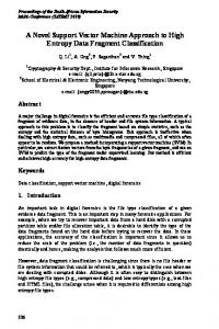
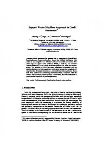
Kernel Functions We can clearly state that kernel functions focus on local neighborhoods around one argument vector, and disregard the effects of points lying far away. In contrast, polynomial kernels give equal weight to all examples in a training sample, and as such exhibit global behavior. The global vs local distinction in kernel behavior can be made more evident through an artificial problem. Assume a sample drawn from two overlapped bivariate Gaussian distributions (each of size n = 1000); each Gaussian corresponds to a different class (positive or negative). An illustration of such artificial setting is shown in Figure 1-left. We will refer to three different reference points to evaluate the behavior of the kernel functions: points A and B, with high class posteriors, and point C with low class posteriors. If we fix one of the three points above as the first argument in the kernel function, and use all other points along the horizontal line from left to right as the second argument, we would observe the plots shown in Figure 1-middle (polynomial kernel) and Figure 1-right (Gaussian kernel). This information can be exploited to predict the success or failure of a kernel function based on data set characteristics.

Introduction Kernel methods have gained increased popularity in the machine learning community in recent years; one key strength underlying these methods is the ability to map the original training points into a higher dimensional feature space, thereby facilitating the job of a low capacity (linear) learning machine. Mapping points into high dimensional spaces has proved an effective strategy for classification in learning algorithms like Support Vector Machines (SVM), mainly because the mapping does not imply an increase in the complexity of the classifier, and because it is possible to rely on an artifice known as the kernel trick, that obviates a precise definition of the mapping functions. The recent success of kernel classification methods has prompted the design of several techniques that aim to improve performance; but only a few studies have focused on understanding the role that the kernel function plays in them. Such information is stored in the gram matrix, or kernel matrix. A kernel matrix has size n × n, where n represents the number of elements in the data set; each entry stands as the dot product of a pair of training elements mapped into a high dimensional space. Past work proposes extracting properties from this matrix to perform kernel selection (Chen et al. 2006; You, Hamsici, and Martinez 2011), using three main metrics: Fisher’s Discriminant, Bregman’s Divergence, and Homoscedasticity. Our study focuses on two of the most used kernel functions: the polynomial and the Gaussian kernels. We analyze

Data Complexity Measures in Kernel Selection To begin, we try to capture the different degrees of data locality based on the clusterability of the data using T 1 measure (obtained from data complexity library DCol). T 1 captures the ratio of clusters to the size of the dataset (clusters are hyper-spheres built through an iterative process using a symmetrical relationship function). A value of T 1 = 1 indicates each training element is a cluster, pointing to the difficulty of finding local neighborhoods. Another data complexity measure, L2 − N 3 (OceguedaHernandez and Vilalta 2013), computes the expected performance gain (Neighborhood Expected Gain N EG) when a local based classifier (Nearest Neighbor) is preferred over a global classifier (linear classifier).

c 2014, Association for the Advancement of Artificial Copyright  Intelligence (www.aaai.org). All rights reserved.

3138

Figure 1: Left. Artificial data set with positive class in red (+) and negative class in blue (). Middle and Right. The behavior of the polynomial and Gaussian kernel functions when applied to the artificial data set in combination with three different reference points: A (black solid line), B (red dashed line), and C (green dotted line).

Figure 2: Decision tree model that predicts a kernel family based on data complexity metrics. Our approach to kernel selection using data complexity measures generates a simple decision tree model (see Figure 2) using T 1 and N EG. We selected data sets with two classes, no missing data, and numeric attributes. After computing T 1 and N EG, we trained our decision tree model to predict the kernel family with best classification performance (see Table 1).

Dataset

T1

NEG

Predicted kernel

Best kernel

Arcene

1

-0.14

Polynomial

Polynomial

Haberman

0.931

-0.068

Gaussian

Gaussian

Hill Valley

1

0.08

Gaussian

Gaussian

Ionosphere

0.946

-0.014

Gaussian

Gaussian

Musk

0.999

0.025

Gaussian

Gaussian

Spambase

0.961

0.082

Gaussian

Gaussian

SPECTF

1

-0.101

Polynomial

Polynomial Gaussian

Blood

0.985

-0.187

Gaussian

Breast Cancer

0.998

0.002

Gaussian

Gaussian

Bank Marketing

1

-0.013

Polynomial

Gaussian

Census Income

0.998

-0.028

Gaussian

Gaussian

Voting Records

1

-0.048

Polynomial

Polynomial

Credit Approval

0.995

-0.049

Gaussian

Gaussian

Bands

1

0.09

Gaussian

Gaussian

Echocardiogram

0.968

0.177

Gaussian

Polynomial

Fertility

0.98

-0.01

Gaussian

Gaussian

Hepatitis

1

-0.038

Polynomial

Polynomial

Sonar

1

0.058

Gaussian

Gaussian

Tic-tac-toe

1

0.021

Gaussian

Gaussian

Table 1: Values of data complexity measures T1 and NEG, and the predicted kernel given by our approach. The last column shows the actual bets approach; bold labels indicate a difference with our prediction.

Conclusions Despite the popularity of kernel methods, there is not yet a mechanism in place that can serve to guide the selection of the kernel function. The goal of this study is to analyze the behavior of polynomial and Gaussian kernels in SVMs, and determine the kernel function that seems best suited for a specific task. To achieve this goal, we analyzed and characterized data sets using data complexity measures. Our approach is guided by the performance of SVMs on several real world dataset, by metrics capturing data properties, and by an estimate of the performance gain of a local classifier over a linear classifier.

lection and boosting with fisher ratio class separability measure. IEEE Transactions on Neural Networks 17(6):1652– 1656. Ho, T. K., and Basu, M. 2002. Complexity measures of supervised classification problems. IEEE Transactions on Pattern Analysis and Machine Intelligence 24(3):289–300. Ocegueda-Hernandez, F., and Vilalta, R. 2013. An empirical study of the suitability of class decomposition for linear models: When does it work well? In 13th SIAM International Conference on Data Mining, 432–440. Austin, TX, USA: Curran Associates. You, D.; Hamsici, O. C.; and Martinez, A. M. 2011. Kernel optimization in discriminant analysis. IEEE Transactions on Pattern Analysis and Machine Intelligence 33(3):631–638.

References Chen, S.; Wang, X. X.; Hong, X.; and Harris, C. J. 2006. Kernel classifier construction using orthogonal forward se-

3139