A Decision Support System for Software Project ... - Semantic Scholar

A Decision Support System for Software Project Management 学术搜索 Software engineering projects are complex sociotechnical systems whose behavior is the result of many technical and human factors, from personnel skills to development tools and processes to business goals. Project managers must identify the right combination of these factors to obtain the desired results. In many fields, managers get support from sophisticated decision support systems, but these haven't yet entered the software engineering mainstream. A hybrid modeling approach can quickly produce process models that can provide project managers accurate predictions, help them design the desired project trajectory, and validate process changes. The NASA Software Engineering Laboratory process provides a case study.Donzelli, P.Software, IEEE67-75July-Aug. 2006学术搜索

scholar search www.libsou.com

feature tools

A Decision Support System for Software Project Management Paolo Donzelli, University of Maryland

Hybrid process modeling can provide project managers with accurate predictions and help them design the project trajectory and validate process changes.

ecision support systems combine individuals’ and computers’ capabilities to improve the quality of decisions.1 Usually adopted in manufacturing to design floor plans and optimize resource allocation and performance, DSSs are penetrating increasingly complex application areas, from insurance fraud detection to military system procurement to emergency planning.2 Although researchers have suggested many approaches,3–8 DSSs haven’t

D


yet entered the main stream of software engineering tools. The complexity of the software process and its sociotechnical nature are often mentioned as the main obstacles to their adoption. As DSSs are developed for other equally complex application areas, we need to identify approaches that can overcome these difficulties and enable project managers to exploit DSSs’ capabilities in their daily activities. A hybrid two-level modeling approach is a step in this direction.

Applying DSSs to software engineering In emergency planning, decision makers must deal with technical and human factors such as unpredictable disaster characteristics (for example, an earthquake’s magnitude, duration, and epicenter), people’s behavior under stress, and potential domino effects resulting in addi-

0740-7459/06/$20.00 © 2006 IEEE

http://www.libsou.com 学术搜索

tional instability (such as power outages). In this context, decision makers adopt DSSs to perform sophisticated what-if analyses, design the best recovery plans (for example, escape routes and resource allocation), and validate interventions (such as transferring emergency personnel among locations) before applying them. DSSs’ capabilities—accurate prediction in an unstable environment, support of trajectory design, and validation of interventions— would benefit software engineering project managers.

Accurate prediction in an unstable environment Before starting a project, the manager could accurately estimate dynamic project behavior (for example, staffing, schedule, effort, and product quality). DSSs would also be useful in case of variable external conditions (such as changing requirements).

July/August 2006

IEEE SOFTWARE

67

Shaping the project trajectory

In software engineering, it’s well known that simple actions can produce counterintuitive feedback.

The manager could shape the project’s behavior by choosing the right combination of development and quality-assurance activities and correctly allocating effort and resources to better meet business goals. For example, the manager could make sure to ■ ■ ■

use most of the effort before a certain date to release staff to other projects, reach the testing phase at a time when necessary resources will be more available, or achieve a certain level of quality as soon as possible to have a product suitable to fill a market opportunity by a controlled release.

Validating interventions Projects can derail because of unexpected events, such as a personnel strike, a new technology’s unpredicted low performance, or an outsourcer’s delay in delivering a component. Additionally, business concerns might demand a change in trajectory (for example, you might need to shorten the delivery time because a competing product is going to market sooner than expected). In any of these scenarios, project managers must act. Before acting, however, they must be sure that their actions will lead to the desired results. In software engineering, it’s well known that simple actions can produce counterintuitive feedback (for example, adding people to a late project could make it even later).9 So, for example, a project manager could check that adopting an extra review activity won’t result in a schedule overrun. A testing manager could verify staff availability before committing himself or herself to higher defect-reduction targets. A process designer could estimate the process overhead that introducing higher concurrency levels among process activities could generate.

let project managers quickly estimate specific project attributes (such as delivery time or effort) or obtain snapshots of the process behavior over time given initial fixed conditions (such as requirements size). Examples include ■ ■ ■

COCOMO,11 to estimate delivery time and effort, Rayleigh,9 to predict and shape the staffing profile, and reliability growth models,12 to estimate the testing required to achieve the desired product quality.

To obtain the required capabilities from an advanced DSS, we must turn to more complex mathematical models, which can’t be analytically solved but require simulation techniques.13 In this case, calculations indicated by the model’s equations are performed over and over to represent the passage of time. If calculations are performed along the time scale at a fixed interval (for example, every second), we have continuous simulation, as with system dynamics models3–5; if they’re performed only when specific events happen (for example, termination of an activity), we have discreteevent simulation, as with queuing network models.6,14 Although either technique can successfully model almost any process aspect, each has advantages and disadvantages.13 Discrete-event models highlight the process’s structure, capturing its components and the entities flowing among them. So, they allow efficient representation of a software process structure in terms of activities and exchanged artifacts and tend to be convenient for detailed process analysis. They’re CPU efficient because computation occurs only when relevant events happen, but they can’t represent continuously varying process variables (such as staff availability). Continuous models, on the other hand, represent a process as a set of equations capturing relationships among dynamic variables of interest (programmer skill, staff availability, final defect density, and so on), although those variables aren’t individually traced through the process. Although these models can easily represent continuously changing variables, they might have difficulty representing process activities. They’re more suitable for strategic long-term analysis than for detailed analysis of a software project.13


Software process models and simulation Process models are a promising means to understand, predict, manage, and improve the software process.10 Different types of models have different capabilities and degrees of complexity. At the bottom level in terms of capability and complexity are analytical models—that is, mathematical models expressed by analytically computable equations. The software community widely adopts these models because they 68

IEEE SOFTWARE

w w w . c o m p u t e r. o r g / s o f t w a r e


Because no single approach is well suited to representing all process aspects, the combination of continuous and discrete-event simulation—that is, hybrid simulation—is emerging as a promising approach.7,8 For example, Robert Martin and David Raffo present a model that represents software development as a series of discrete steps, executed in a continuously varying project environment.7

A hybrid modeling approach I propose exploiting the advantages of the three traditional modeling methods (analytical models and continuous and discrete-event simulation) by combining them into a hybrid two-level modeling approach.8 At the higher abstraction level, the process is modeled as a discrete-event queuing network— that is, a set of service stations that process customers. A typical example of a queuing network is a set of superstore checkout counters (service stations) with customers queuing up to pay. A customer arrives at a station to obtain a service, waits in line if the station is serving another customer, and leaves after being served. A queuing network provides a natural way to represent a software process structure, its activities, their interactions, and the exchanged artifacts. The process activities (design, coding, testing, and so on) can be represented as service stations. The circulating artifacts (design documents, code, faults reports, and so on) can be represented as customers moving from one service station to another (for example, a design document moving from the design to the testing activity). At the lower abstraction level, analytical models and continuous simulation represent the dynamic behavior of the service stations introduced at the higher abstraction level. I implemented the suggested approach using the Queuing Networks Analysis Package 2.15 Although I could have adopted any package, QNAP2 provides convenient language primitives to support the hybrid model’s development.

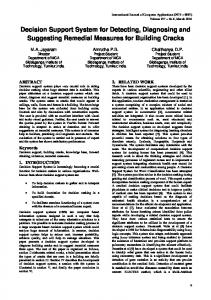
product size, process staffing profile, staffing profiles over single activities, defect patterns, and so on). As figure 1 shows, the SEL software process consists of a series of phases: specification (SP), high-level design (HLD), low-level design (LLD), implementation (IMP), system test (ST), and acceptance test (AT). The final software product is the end result of a series of main artifacts: requirements, specification, high-level design, low-level design, code, system-tested code, and acceptance-tested code. Although the phases are sequential, their respective activities can run concurrently, given the simultaneous execution of work tasks that generate the main artifacts and rework tasks to fix defects or introduce requirement modifications. So, in addition to the main artifacts, artifacts are also generated and dealt with by tasks aiming at fixing defects (LLD defects reports, code correction reports, and so on) and by tasks that introduce modifications due to requirements instability (such as SP changes and HLD increments).

Because no single modeling approach is well suited to representing all process aspects, hybrid simulation is emerging as a promising approach.

Modeling the SEL software process

scholar search

My hybrid approach translates the SEL software process into a two-level model. At the higher abstraction level, I model the process as a queuing network (see figure 2 on page 71). A set of service stations, each representing an internal task (for example, development of the main artifact, review, and defect correction), models process activity. In particular, I’ve used two different types of subnetworks to model the development activities (SP, HLD, LLD, and IMP) and the testing activities (ST and AT). For example, figure 2 highlights the subnetworks that model the HLD and AT activities. The subnetwork that models the HLD activity has these main service stations:

www.libsou.com

The NASA Software Engineering Laboratory process As a case study, I used this hybrid approach to model the NASA SEL software process.16,17 The model focuses on the main process quality attributes (effort, delivery time, productivity, rework percentage, and product defect density) and numerous subattributes (final


■ ■

■

■

The work station models the HLD’s development on the basis of the received SP. The external rework station simulates the activity necessary to modify the HLD on the basis of the received SP changes and increments and produces the corresponding HLD changes and increments. The review station simulates the review performed on the HLD and HLD changes and increments. The internal rework station simulates the

July/August 2006

IEEE SOFTWARE

69

Requirements Requirements changes Requirements increments

SP defects reports Specification (SP) activity

Specification SP changes SP increments SP corrections reports

HLD defects reports High-level design (HLD) activity

Process activities

High-level design HLD changes HLD increments HLD corrections reports

LLD defects reports

Low-level design LLD changes LLD increments LLD corrections reports

Low-level design (LLD) activity Code defects reports

Code Code changes Code increments Code corrections reports

Implementation (IMP) activity

System test (ST) activity

System-tested code System-tested code changes System-tested code increments System-tested code corrections reports

Acceptance test (AT) activity

scholar search Process phases

www.libsou.com SP HLD

LLD

IMP

ST

activity necessary to fix the HLD on the basis of the received SP corrections reports and HLD defects reports. It then generates the corresponding HLD corrections reports. Similarly, the subnetwork that models the AT activity has these main service stations: ■ ■

The work testing station simulates acceptance testing of the system-tested code. The external rework testing station simulates acceptance testing of the systemtested code changes and increments.

In both these networks, the remaining service stations coordinate artifact flow: ■ ■

70

IEEE SOFTWARE

The start station routes the input artifacts toward the appropriate service station The release and store stations handle the



Defects reports

Figure 1. The NASA Software Engineering Laboratory software process.

AT

Acceptance-tested code Acceptance-tested code changes Acceptance-tested code increments (Final SW product)

Time

release of the output artifacts. For example, in the HLD activity, the HLD artifact will be released only after all the defects discovered during the review have been corrected. At the lower abstraction level, each service station in figure 2 is modeled by a combination of analytical models and continuous simulation. In particular, depending on the specific task that the service station simulates, I’ve adopted a different set of analytical models, derived from SEL guidelines,14 to express the corresponding required resources (for example, time and personnel) and performances (such as defect injection during development, defect detection during review, and productivity). For example, figure 3 shows some implementation details of the HLD work station. This station starts operating when it receives

Requirements Requirements changes Requirements increments

Specification SP changes SP increments SP correction reports

SP

HLD defects reports (due to locally injected defects)

Start station

Work station

Review station

Release station

SP defects reports

External rework station

HLD

Store station Internal rework station

High-level design HLD changes HLD increments HLD correction reports LLD

scholar search

Legend: Service station Subnetwork used to model a process activity

IMP

www.libsou.com

LLD

Circulating artifacts

ST System-tested code ST code changes ST code increments ST code correction reports AT code defects reports Start station

AT

Work station

Release station

External rework station Store station Acceptance-tested code AT code changes AT code increments (Final SW product)

Figure 2. The higher abstraction level: queuing network of the SEL software process.


July/August 2006

IEEE SOFTWARE

71

On the basis of T and W, the staff necessary over time to produce the HLD artifact is represented using the Rayleigh model. Here, continuous simulation is adopted. The staff required each week for the development task is obtained by computing at a one-week interval (that is, the simulation interval) the Rayleigh equation:

Continuous simulation Staffstaff E (t )

0.39W

t2 t − 2T 2 E (t ) = W e T2

T Time (Rayleigh model computed at 1-week intervals)

2

E (t ) = W Specification artifact

High-level design artifact Size: HLD_size Effort: WSP + 0.39W

size: SP_size effort: WSP Work station

Analytical models COCOMO-like size estimator b HLD _ size = Random (a1SP_ size 1+ c1 ) COCOMO-like Time estimator b

T = a2HLD _ size 2 + c 2 COCOMO-like effort estimator b

Wtot = a3HLD _ size 3 + c3

Figure 3. Modeling the lower abstraction level: details of the workstation in the high-level design activity.

72

IEEE SOFTWARE

t − t2 e 2T T2

According to the Rayleigh model, the output artifact is released at time T—that is, when the staff level E(t) peaks. So, to produce the HLD artifact, the work station uses only a percentage of the development effort computed through the COCOMO-like effort estimator (that is, the integral up to T, as in figure 3). This percentage (0.39W) is then added to the effort of the specification (WSP) to obtain the effort attribute of the HLD (WSP + 0.39W). The C OCOMO -like estimators used to model the work service stations in the different activities have been derived from SEL data.16,17 In particular, I combined the original SEL COCOMO models with the observed effort distribution across the various SEL process activities.

scholar search the SP artifact (the input customer) and simulates the development of the HLD artifact (the output customer). As schematized in figure 3, two attributes describe artifacts: size and effort. According to the SEL, the size of the SP and HLD artifacts are expressed in SP and HLD units.6,12 Effort (measured in person-weeks) represents the accumulated effort—that is, the effort that the staff has spent to develop the artifact since the process’s beginning. On the basis of the SP artifact’s attributes, the work station computes the corresponding HLD artifact attributes and simulates the development task’s dynamic behavior in terms of delivery time and required staff. First, starting from the specification’s size (SP_size), a COCOMO-like estimator calculates the HLD’s size (HLD_size). Because such a quantity might have random deviations in real life, a Gaussian pseudorandom generator transforms the average size into the corresponding random value. Then, two other COCOMO-like estimators compute the delivery time (T) and the development effort (W).



A decision support tool for the manager

www.libsou.com

To illustrate the simulation model’s capabilities as a DSS, I’ve used it to study how requirements instability affects a project. I applied the model to reproduce two possible software development scenarios: ■

■

a stable-requirements scenario, wherein a requirements artifact of 1,500 function points is fed to the process model, and an unstable-requirements scenario, wherein the initial requirements artifact of 1,500 function points is followed by requirements increments and changes regularly fed into the process over the development time to reproduce a situation in which requirements grow by 20 percent and change by 15 percent.

Table 1 and figures 4 and 5 show the simulation results for the stable-requirements scenario. Table 1 shows the predicted average values for product size, development effort, delivery time, productivity, rework percentage, defects density,

Table 1 Stable requirements: Simulation results vs. SEL data SW process attribute

SEL data are within or very close to the confidence interval the simulator provided.

Simulation results Average values

Confidence interval (95%)

SEL data

Final product size

116 KLOC

N/A

116 KLOC

Effort (W)

500 person-weeks

440–560 person-weeks

600 person-weeks

Delivery time (T)

78 weeks

75–81 weeks

63 weeks

Productivity

5.8 LOC/person-hour

4–7.6 LOC/person-hour

5.3 LOC/person-hour

Rework percentage

17%

14–21%

Not available

Defect density

0.9 defects/KLOC

0.6–1.2 defects/KLOC

Not available

Average number of staff

6.5

5.5–7.5

9.5

15

12 Number of staff

and staff. It also shows the corresponding confidence intervals—that is, the intervals that the model predicts the results will be within in 95 percent of the cases. Figure 4 shows the staff profile for the whole project, and figure 5 details the staff profile for the IMP activity. Both figures show the average value within its 95 percent confidence interval. We can now investigate these results’ validity. A simulation model’s validity is usually verified by comparing simulation results quantitatively and qualitatively against real-world data and by demonstrating the model’s ability to reproduce empirically known facts (for example, requirements instability’s effects on a process). To compare the simulation results against real data, table 1’s SEL data column shows the data obtained with the available SEL estimation models16,17 for a software product of 116 KLOC. This comparison’s results are comforting, because SEL data are within (in one case) or very close to the confidence interval the simulator provided. In addition, the staff behavior that figures 4 and 5 illustrate indicates the simulation results’ closeness to real-world SEL data. In both cases, staff profiles behave as expected for an SEL project: The average staff profile for the entire project (figure 4) strongly resembles the trapezoidal shape (compare with figure 6), while the staff profile for a single activity (figure 5) is very similar to a Rayleigh curve (the dotted line in figure 5). To verify the model’s ability to reproduce empirically known facts, we can turn to the simulation results for the scenario with unstable requirements. Figure 7 illustrates the effects of requirements instability on the staffing profile and compares the profiles for stable and

9

6

scholar search


3

0 0

9

18

27

36

45 54 Week

www.libsou.com

63

72

81

90

99

Figure 4. Stable requirements: staffing profile for the whole project.

15

Number of staff

12

9

6

3

0 0

6

12 18 24 30 36 42 48 54 60 66 72 78 84 90 96 Week

Figure 5. Stable requirements: staffing profile for the implementation activity.

July/August 2006

IEEE SOFTWARE

73

Detailed design

Requirements analysis

Preliminary design

26

System delivery

System testing Implementation

Acceptance testing

22

Staff

18

14

10 Second replan First replan Initial plan Actual data

6

2 0

10

20

30

40

50

60 Week

70

80

90

100

110

120

Figure 6. SEL staffing profile for a project with high requirements instability.16,17

15

scholar search

12

Stable

T www.libsou.com Unstable

Staff

9

6

3

0

1

15

Figure 7. Project staffing profile for stable vs. unstable requirements.

74

and the final product’s defect density has increased (+66 percent). In addition, simulation results allow for an interesting comparison with real SEL project behavior. The behavior of the simulator-generated staffing profile is qualitatively very similar to that of the staffing profile (figure 6) SEL measured for a project with similar characteristics (that is, a slightly larger product size, 160 KLOC rather than 140 KLOC, and high requirements instability). Although the original SEL data show that managers had to replan twice during the project to fit its dynamics (that is, first and second replan to fit the actual data), the simulation model can estimate the process dynamics with only one application. Project managers can simulate different possible unstable scenarios (that is, different kinds of requirements behavior over time) to estimate the corresponding project trajectories. So, managers will not only have accurate predictions in unstable environments but also be able to manage the new requirements over time (that is, to decide when and how to feed them to the project) to design a trajectory that better fits the organizational needs.

IEEE SOFTWARE

29

43

57 71 Week

85

99

113

127

unstable requirements. The simulator confirms the empirical expectation that requirements instability leads to a substantial increase of effort and delivery time (38 and 60 percent, respectively). It also confirms the expected reduction of process productivity, increased rework percentage, and worsening of the final product quality (defect density). In fact, the rework percentage has more than doubled (+150 percent), productivity has clearly dropped (-21 percent),



his case study demonstrates that the hybrid modeling approach can provide both qualitative and quantitative suggestions on tuning the software process to improve its quality and better meet organizational needs. Combining three traditional modeling methods overcomes some of the limits of the individual approaches (for example, analytical models’ limited estimation capabilities). It also provides some clear advantages. First, it lets you bridge the gap between modelers and project managers. It allows exploiting the graphical clarity of queuing networks and project managers’ familiarity with analytical models such as COCOMO and Rayleigh. Also, it allows quick reuse of knowledge available in organizations. A queuing network, in fact, can be obtained as a direct replica of the process structure often described in organizational standards, and analytical models are commonly adopted within a software company to manage projects. Finally, it results in flexible process models, easily adaptable to the organization’s character-

About the Author

istics and maturity level and updateable to follow its evolution (as advocated by software process improvement methods such as the Capability Maturity Model18 or the Quality Improvement Paradigm19). You can easily change or update the queuing network and its embedded analytical models to address the specific context needs.

Paolo Donzelli is the director of the Research and Information and Communication Technologies Division of the Department for Innovation and Technology of the Office of the Prime Minister of Italy. He’s also a visiting senior research scientist in the University of Maryland’s Computer Science Department. His research interests include software process improvement, requirements engineering, and dependability modeling and validation. He received his PhD from the University of Rome Tor Vergata. Contact him at the Dept. of Computer Science, Univ. of Maryland, College Park, MD 20742; [email protected].

Acknowledgments

9. L.H. Putnam and W. Meyer, Measures for Excellence: Reliable Software on Time within Budget, Prentice Hall, 1992. 10. A. Finkelstein, J. Kramer, and B. Nuseibeh, eds., Software Process Modeling and Technology, John Wiley & Sons, 1994. 11. B.W. Boehm, Software Engineering Economics, Prentice Hall, 1981. 12. S.H. Kan, Metrics and Models in Software Quality Engineering, Addison-Wesley, 1994. 13. M. Kellner, R. Madachy, and D. Raffo, “Software Process Simulation Modeling: Why? What? How?” J. Systems and Software, vol. 46, no. 2/3, 1999, pp. 201–219. 14. D. Gross and C. Harris, Fundamentals of Queuing Theory, John Wiley & Sons, 1998. 15. SIMULOG, QNAP2 User Guide ver. 9.3, Simulog, 1986. 16. L. Landis et al., Recommended Approach to Software Development (Revision 3), tech. report SEL-81-305, Software Eng. Laboratory, NASA-GSFC, 1992. 17. M.Bassman, F. McGarry, and R. Pajerski, Software Measurement Guidebook, tech. report SEL-94-002, Software Eng. Laboratory, NASA-GSFC, 1994. 18. M.C. Paulk et al., The Capability Maturity Model for Software, Software Eng. Inst., Carnegie Mellon Univ., 1993. 19. V.R. Basili, G. Caldiera, and H.D. Rombach, “The Experience Factory,” Encyclopedia of Software Eng., John Wiley & Sons, 1994.

I completed part of this work as a PhD student in the Computer Science Department of the University of Rome Tor Vergata.

References 1. G.M. Marakas, Decision Support Systems in the 21st Century, Prentice Hall, 2003. 2. R.C. Dorf, Technology, Humans, and Society, Academic Press, 2001. 3. T.K. Abdel-Hamid and S.E. Madnick, Software Project Dynamics: An Integrated Approach, Prentice Hall, 1991. 4. “What is System Dynamics,” System Dynamics Soc., 2006, www.systemdynamics.org. 5. G.F. Calavaro, V.R. Basili, and G. Iazeolla, “Simulation Modeling of Software Development Process,” Proc. 7th European Simulation Symp., Soc. for Computer Simulation, 1995. 6. G.A. Hansen, “Simulating Software Development Processes,” Computer, vol. 29, no. 1, 1996, pp. 73–77. 7. R.H. Martin and D. Raffo, “A Model of the Software Development Process Using both Continuous and Discrete Models,” Int’l J. Software Process Improvement and Practice, vol. 2, no. 2/3, 2000, pp. 147–157. 8. P. Donzelli and G. Iazeolla, “Hybrid Simulation Modelling of the Software Process,” J. Systems and Software, vol. 59, no. 3, 2001, pp. 227–235.


ADVERTISER Advertiser

INDEX

JULY/AUGUST

Page Number

Addison-Wesley EclipseWorld 2006 ICSM 2006 John Wiley & Sons LinuxWorld Conference & Expo 2006 RE 2006 SD Best Practices Conference & Expo 2006 Boldface denotes advertisements in this issue.

21 1 18 Cover 2 13 10 Cover 4

2006

Advertising Personnel Marion Delaney IEEE Media, Advertising Director Phone: +1 415 863 4717 Email: [email protected] Marian Anderson Advertising Coordinator Phone: +1 714 821 8380 Fax: +1 714 821 4010 Email: [email protected]

Sandy Brown IEEE Computer Society, Business Development Manager Phone: +1 714 821 8380 Fax: +1 714 821 4010 Email: [email protected]

Advertising Sales Representatives Mid Atlantic (product/recruitment) Dawn Becker Phone: +1 732 772 0160 Fax: +1 732 772 0164 Email: [email protected] New England (product) Jody Estabrook Phone: +1 978 244 0192 Fax: +1 978 244 0103 Email: [email protected] New England (recruitment) John Restchack Phone: +1 212 419 7578 Fax: +1 212 419 7589 Email: [email protected] Connecticut (product) Stan Greenfield Phone: +1 203 938 2418 Fax: +1 203 938 3211 Email: [email protected]

Midwest (product) Dave Jones Phone: +1 708 442 5633 Fax: +1 708 442 7620 Email: [email protected] Will Hamilton Phone: +1 269 381 2156 Fax: +1 269 381 2556 Email: [email protected] Joe DiNardo Phone: +1 440 248 2456 Fax: +1 440 248 2594 Email: [email protected] Southeast (recruitment) Thomas M. Flynn Phone: +1 770 645 2944 Fax: +1 770 993 4423 Email: [email protected]


Midwest/Southwest (recruitment) Darcy Giovingo Phone: +1 847 498-4520 Fax: +1 847 498-5911 Email: [email protected] Southwest (product) Steve Loerch Phone: +1 847 498 4520 Fax: +1 847 498 5911 Email: [email protected] Northwest (product) Peter D. Scott Phone: +1 415 421-7950 Fax: +1 415 398-4156 Email: [email protected] Southern CA (product) Marshall Rubin Phone: +1 818 888 2407 Fax: +1 818 888 4907 Email: [email protected]

Northwest/Southern CA (recruitment) Tim Matteson Phone: +1 310 836 4064 Fax: +1 310 836 4067 Email: [email protected] Southeast (product) Bill Holland Phone: +1 770 435 6549 Fax: +1 770 435 0243 Email: [email protected] Japan Tim Matteson Phone: +1 310 836 4064 Fax: +1 310 836 4067 Email: [email protected] Europe (product) Hilary Turnbull Phone: +44 1875 825700 Fax: +44 1875 825701 Email: [email protected]