detect performance bottlenecks and deadlocks in both software and hardware. .... Service calls can be made from entries in one task to entries in other tasks.
A DEVS LIBRARY FOR LAYERED QUEUING NETWORKS Dorin B. Petriu and Gabriel Wainer Department of Systems and Computer Engineering Carleton University, 1125 Colonel By Drive Ottawa, Ontario K1S 5B6, Canada. {dorin | gwainer}@sce.carleton.ca
ABSTRACT
2. BACKGROUND
The DEVS formalism is a modeling and simulation framework with well-defined concepts for coupling components and the construction of hierarchical modular models. Different formalisms, including Petri Nets, PDE, and state machines, have been mapped into DEVS. In this paper, a Layered Queuing Network (LQN) library is developed and mapped into DEVS using the CD++ toolkit. LQNs are used for performance analysis of software systems. LQNs can model multilayer client-server applications, and as such they can be used to detect performance bottlenecks and deadlocks in both software and hardware. This paper shows how to build LQNs as DEVS models, thus integrating between the two kinds of models, and providing a framework for defining complex models through the use of multiformalism modeling.
A real system modeled with DEVS is described as a composite of submodels, each of them being behavioral (atomic) or structural (coupled).
Keywords: DEVS, LQN, CD++, multiformalism model, performance analysis
1. INTRODUCTION The DEVS formalism [1] is a discrete-event modeling specification mechanism based on systems theory, which supports the definition of hierarchical modular models that can be easily reused. DEVS hierarchical constructions enable multi-formalism modeling; that is, the coupling of and transformation between models described in different formalisms. Using different formalisms to represent systems enables a modeler to choose the best formalism for each sub-system. The CD++ [2] tool allows the user to implement DEVS models. CD++ is built as a hierarchy of models, each related to a simulation entity. Atomic models can be programmed in C++. A specification language exists for defining a model's interfaces to other models and for defining a model’s initial values and external events. The tool also enables a user to build models using graph-based notations, which allows for a more abstract visualization of the problem, as well as for the definition of cellular models. In the long term, the goal is to provide users with a set of libraries to develop complex models based on multiformalisms. There already are libraries for Finite State Automata, Petri Nets, DEVS graphs, and DEVS atomic models written in C++. In this work we show how to define Layered Queuing Networks (LQNs) [3, 4] in a DEVS environment. LQNs are built as client/server models that triggered by discrete events. They are provided with modular entry points and the layered definition permits hierarchical construction. This paper shows that the mapping of LQNs into DEVS models is straightforward.
A DEVS atomic model is formally described by: M = < X, S, Y, δint, δext, λ, D > where X is the input events set; S is the state set; Y is the output events set; δint is the internal transition function; δext is the external transition function; λ is the output function; and D is the duration function. Each model is provided with an interface consisting of input and output ports to communicate with other models. Input external events (those events received from other models) are collected in input ports. The external transition function specifies how to react to those inputs. The internal transition function is activated after a period defined by the time advance function. The goal is to produce internal state changes. Model execution results are spread through output ports. This is done by the output function, which executes before any internal transition A DEVS coupled model is composed of several atomic or coupled submodels. They are formally defined as: CM = < X, Y, D, {Mi}, {Ii}, {Zij} > where X is the set of input events; Y is the set of output events; D is an index for the components of the coupled model, and ∀ i ∈ D, Mi is a basic DEVS (that is, an atomic or coupled model), Ii is the set of influencees of model i (that is, the models that can be influenced by outputs of model i), and ∀ j ∈ Ii, Zij is the i to j translation function. Queuing Networks are based on a customer-server paradigm: customers request service to servers, which queue the requests until they can be serviced. Traditional Queuing Networks model only a single layer of customer-server relationships. LQNs allow for an arbitrary number of clientserver levels. LQNs can model intermediate software servers, and be used to detect software deadlocks and software as well as hardware performance bottlenecks [5]. The layered aspect of LQNs makes them very suitable for evaluating the performance of distributed systems [6, 7]. LQNs model both software and hardware resources. The basic software resource is a task, which represents any software object having its own thread of execution. Tasks have entries that act as service access points. The basic hardware resource is a device. Typical devices are CPUs and disks [8]. Figure 1 shows the visual notation used for tasks, entries, and devices.
made in sequence. Figure 3 shows the time semantics of these different types of calls.
Figure 1. LQN task, entry, CPU and disk devices. Tasks receive service requests at designated interface points called entries. Entries correspond to service access point for a task. There is a different entry for every kind of service that a task provides. An entry may be defined atomically, with its own hardware service demands and calls to other tasks. Alternately, an entry may be defined by blocks of smaller computational blocks called activities. An entry receiving a synchronous service call is responsible for sending a reply after the request has been completed. Replies are implicit at the end of the first phase for entries that are defined atomically, but must be explicitly specified for entries defined by activities. An entry receiving a synchronous service request may also forward it to entries in other tasks which then become responsible for sending the reply to the original caller. In the case of a forwarded call, the original calling task remains blocked until it finally receives the reply at the end of the forwarding chain. Service calls can be made from entries in one task to entries in other tasks. Entries can be atomic or subdivided into phases that divide the workload into a first phase that is executed prior to sending a reply and a second phase that is executed after sending a reply. Service calls are shown by messaging arrows. The LQN notation supports three types of calls: asynchronous, synchronous, and forwarded calls, as shown in Figure 2.
The LQSim simulator [9] was built to solve LQNs via means of simulation. LQSim was built using the ParaSol simulation environment, which can simulate multithreaded systems that support transactions and provides built-in statistics for monitoring simulation objects [10]. LQNs are simulated by creating tokens for each call and following those tokens through the system. The performance metrics are arrived at by recording the wait times and other statistics for each to-ken. The simulator generates results showing average entry service times, average waiting time, throughput, and utilization, as well as processor throughput and utilization.
Figure 3. Time semantics of LQN calls The LQSim provides facilities to model LQNs, but we want to go a step further by providing means to make queuing networks to interact with models written in other formalisms. For instance, we could define a DEVS model describing dynamic behaviour based on the metrics obtained running an LQN describing the system. This model could be integrated with a Petri Net model, which could be used to control the concurrent triggering of a client/server model written using LQNs. We have CD++ to develop libraries for Petri Nets [11], Finite State Automata [12], DEVS Graphs [2] and cellular models [2]. Introducing an LQN library would permit us to integrate the behaviour described by this modeling technique with the one described with other modeling tools.
3. LQN SIMULATION LIBRARY FOR DEVS
Figure 2: LQN messaging. Asynchronous calls do not involve any blocking of the sending task whereas synchronous calls block the sending client task until it receives a reply. In a forwarding call, the sending client task makes a synchronous call and blocks waiting for a reply; the receiving intermediate server task then partially processes the call and forwards it to another server which becomes responsible for sending a reply to the blocked client. The intermediate server can continue operation after forwarding the call (there can be any number of forwarding levels). Calls are made from a task’s entries and they can be
An LQN library must represent processors, tasks, and entries with phases. Additionally, the library might also represent disks and activities. The library should provide results for: • average entry service time, throughput, and utilization • average phase service time • processor throughput and utilization • average queue waiting time, average queue length. The main design issue for the DEVS LQN simulation library was to decide which LQN elements or artifacts to model as DEVS atomic models and which ones to model as DEVS coupled models. Processors, tasks, and entries with phases definitely needed to be included in the library. Activities were initially left out since they are optional in the LQN notation. LQN elements have queues that are implicitly supported by LQNS and LQSim. FIFO queues were incorporated explicitly
into the DEVS LQN library. Since queues behave the same way for software or hardware elements, a decision was made to implement a universal queue as a separate atomic model to be coupled with the processor or entry atomic models.LQN calls are made using entry names to identify the call target. Therefore, a mechanism was needed to deal with addressing the calls in DEVS. The solution was to implement a DEVS version of a multiplexer and demultiplexer to either gather calls into a given queue (either for an entry or a processor) or to distribute calls from an entry to other entries. A DEVS atomic model was built for each of these elements. The complete set of models can be found at http://www.sce.carleton.ca/faculty/wainer/, and here we will briefly introduce the behaviour of some of these models. Figure 4 describes the behaviour of the queue atomic model. The initial state (wait for ready) represents a queue ready to receive request. When an external transition is executed and an external event arrives through the in port, the element is added to the end of the queue. When a ready event arrives, we check if the queue has elements. If not, we change state to ready to process, waiting for a new element arriving through the in port. When this event occurs, or if the queue has elements, we immediately send the first element through the out port, computing also the average size and wait times. Then we go to the state wait for response, in which we wait for a response event (which generates a response in the reply output port), or a new element, which is added at the end of the queue.
of the Queue is connected to the output port of the Gather multiplexer model.
Figure 5. FSM for the DEVS entry atomic model. For entries, the servcall output port is connected to the in port of the Distribute demultiplexer, which sends it on the appropriate out port for the intended call target. The same sort of connections is repeated for the reply ports but with the reply messages going in the opposite direction. These coupled models fully represent the LQN processors and entries.
Figure 4. DEVS queue atomic model. Table 1 (in the Appendix) lists the different DEVS models for LQN elements. The Gather and Distribute models have nonblocking, single-state FSMs that instantly pass messages through and route them to the correct ports. Figure 5 shows the FSM one of the more complex atomic models implemented (the entry atomic model). Figure 6 shows the structure of the DEVS coupled models for LQN Entries and Figure 7 shows structure of the DEVS coupled model for LQN Processors. Both of these coupled models incorporate queues and message routing multiplexers/demultiplexers. The in ports of the Processor and Entry atomic models are connected to the out ports of their dedicated Queue atomic models. The in port
Figure 6. DEVS Entry coupled mode structure. LQN messages can be thought of as having a source field denoting the entity making the call, a destination or target field denoting the entry for which the call is destined, and a demand field denoting the workload associated with the call. Simple DEVS messages have only a single variable field per message,
therefore making it necessary to send and receive sets of two or three messages in order to transmit all of the required fields. Table 2 (in the Appendix) lists the messages sent between atomic models in the DEVS LQN simulation library, how they are ordered, and how they should be interpreted.
server “e2”. Entry1 has a mean processor demand of 1100 ms and entry2 has a mean processor demand of 2100 ms. All three tasks run on the same processor P1. The equivalent LQN is shown in Figure 8 below.
Figure 8. LQN model as defined in CD++.
Figure 7. DEVS Processor coupled model structure.
4. ASSEMBLING DEVS LQN MODELS This section describes the CD++ definition of a model in which each component is defined as an LQN element. [top] components : ref e1 e2 p1 in : refinitp refinits refin e1initp e1inits in : e2initp e2inits link : refinitp initp@ref link : refinits inits@ref link : refin in0@ref link : pcall@ref in0@p1 link : rpl0@p1 prtn@ref link : e1initp initp@e1 link : e1inits inits@e1 link : out0@ref in0@e1 link : rpl0@e1 rsp0@ref link : pcall@e1 in1@p1 link : rpl1@p1 prtn@e1 link : e2initp initp@e2 link : e2inits inits@e2 link : out1@ref in0@e2 link : rpl0@e2 rsp1@ref link : pcall@e2 in2@p1 link : rpl2@p1 prtn@e2
The model defined above shows a test client-server system where the client “ref” calls entry1 in server “e1” and entry2 in
This model was executed using the input events presented in Table 3. As we can see, we start by making phase 1 of entry ent in task “ref” to be initialized to make one call to entry entry1 in task “e1”, and one call to entry entry2 in task “e2” (a call initialization is assembled from three messages; one for the phase making the call, one for the number of calls, and one for the call target). Then, we see that phase 1 of entry entry1 in task “e1” is initialized with a mean workload of 1100 ms, and phase 1 of entry entry2 in task “e2” is initialized with a mean workload of 2200 ms (a processor demand initialization is assembled from two messages; one for the phase, and one for processing workload). Finally, 10 calls are made to entry ent in task “ref” at 1 sec intervals. Input Events
00:00:00:000 00:00:00:001 00:00:00:002 00:00:00:003 00:00:00:004 00:00:00:005 00:00:00:006 00:00:00:007 00:00:00:010 00:00:00:011 00:00:01:000 00:00:02:000 00:00:03:000 00:00:04:000 00:00:05:000 00:00:06:000 00:00:07:000 00:00:08:000 00:00:09:000 00:00:10:000
refinits 1 refinits 1 refinits 0 refinits 1 refinits 1 refinits 1 e1initp 1 e1initp 1100 e2initp 1 e2initp 2100 refin 1 refin 1 refin 1 refin 1 refin 1 refin 1 refin 1 refin 1 refin 1 refin 1
Table 3: Input events for the model defined in Figure 5. Table 4 below shows the execution results of this model.
Model execution [00:00:00:002] entry: init phase1 call stmt 1 = 1 calls to server 0 [00:00:00:005] entry: init phase1 call stmt 2 = 1 calls to server 1 [00:00:00:007] entry: init phase1 proc demand mean = 1100 ms [00:00:00:011] entry: init phase1 proc demand mean = 2100 ms [00:00:01:000] entry: start; entry: phase1 server call [00:00:01:000] entry: start; entry: phase1 proc call ; processor: [00:00:02:087] entry: reply; entry: done ; entry: phase1 server call ; entry: start [00:00:02:087] entry: phase1 proc call [00:00:02:087] processor: [00:00:04:168] entry: reply; entry: done [00:00:04:168] entry: reply; entry: done
Interpretation entries being initialized with their call and workload paramers execution of the first call made to entry ent in task “ref” and subsequent calls to entries entry1 in task “e1” which generates an actual processor workload of 1087 ms and to entry2 in task “e2” which generates an actual processor workload of 2081 ms
[00:00:04:168] entry: start; entry: phase1 server call [00:00:04:168] entry: start; entry: phase1 proc call ; processor: [00:00:05:048] entry: reply; entry: done [00:00:05:048] entry: phase1 server call ; entry: start [00:00:05:048] entry: phase1 proc call [00:00:05:048] processor: [00:00:05:326] entry: reply; entry: done [00:00:05:326] entry: reply; entry: done [00:00:05:326] entry: start; entry: phase1 server call [00:00:05:326] entry: start; entry: phase1 proc call ; processor: [00:00:06:032] entry: reply; entry: done [00:00:06:032] entry: phase1 server call ; entry: start [00:00:06:032] entry: phase1 proc call [00:00:06:032] processor: [00:00:08:122] entry: reply; entry: done [00:00:08:122] entry: reply; entry: done [00:00:08:122] entry: start; entry: phase1 server call [00:00:08:122] entry: start; entry: phase1 proc call ; processor: [00:00:09:281] entry: reply; entry: done [00:00:09:281] entry: phase1 server call [00:00:09:281] entry: start; entry: phase1 proc call ; processor: [00:00:09:696] entry: reply; entry: done [00:00:09:696] entry: reply; entry: done [00:00:09:696] entry: start; entry: phase1 server call [00:00:09:696] entry: start; entry: phase1 proc call ; processor: [00:00:09:703] entry: reply; entry: done [00:00:09:703] entry: phase1 server call ; entry: start [00:00:09:703] entry: phase1 proc call [00:00:09:703] processor: [00:00:10:852] entry: reply; entry: done [00:00:10:852] entry: reply; entry: done [00:00:10:852] entry: start; entry: phase1 server call [00:00:10:852] entry: start; entry: phase1 proc call ; processor: [00:00:15:054] entry: reply; entry: done [00:00:15:054] entry: phase1 server call ; entry: start [00:00:15:054] entry: phase1 proc call [00:00:15:054] processor: [00:00:21:264] entry: reply; entry: done [00:00:21:264] entry: reply; entry: done [00:00:21:264] entry: start; entry: phase1 server call [00:00:21:264] entry: start; entry: phase1 proc call ; processor: [00:00:22:205] entry: reply; entry: done [00:00:22:205] entry: phase1 server call ; entry: start [00:00:22:205] entry: phase1 proc call [00:00:22:205] processor: [00:00:27:364] entry: reply; entry: done [00:00:27:364] entry: reply; entry: done [00:00:27:364] entry: start; entry: phase1 server call [00:00:27:364] entry: start; entry: phase1 proc call ; processor: [00:00:27:909] entry: reply; entry: done ; entry: phase1 server call ; entry: start; entry: phase1 proc call ; processor: [00:00:30:284] entry: reply; entry: done [00:00:30:284] entry: reply; entry: done [00:00:30:284] entry: start; entry: phase1 server call ; entry: start; entry: phase1 proc call ; processor: [00:00:32:540] entry: reply; entry: done ; entry: phase1 server call ; entry: start [00:00:32:540] entry: phase1 proc call [00:00:32:540] processor: [00:00:37:487] entry: reply; entry: done [00:00:37:487] entry: reply; entry: done [00:00:37:487] entry: start; entry: phase1 server call [00:00:37:487] entry: start; entry: phase1 proc call ; processor: [00:00:39:214] entry: reply; entry: done [00:00:39:214] entry: phase1 server call ; entry: start [00:00:39:214] entry: phase1 proc call [00:00:39:214] processor: [00:00:40:088] entry: reply; entry: done [00:00:40:088] entry: reply; entry: done
execution of the second call made to entry ent in task “ref” and subsequent calls to entries entry1 in task “e1” which generates and actual processor workload of 880 ms and to entry2 in task “e2” which generates and actual processor workload of 278 ms Execution of the third call made to entry ent in task “ref” and subsequent calls to entries entry1 in task “e1” which generates an actual processor workload of 706 ms and to entry2 in task “e2” which generates an actual processor workload of 2090 ms execution of the fourth call made to entry ent in task “ref” and subsequent calls to entries entry1 in task “e1” which generates an actual processor workload of 1159 ms and to entry2 in task “e2” which generates an actual processor workload of 415 ms execution of the fifth call made to entry ent in task “ref” and subsequent calls to entries entry1 in task “e1” which generates an actual processor workload of 7 ms and to entry2 in task “e2” which generates an actual processor workload of 1149 ms execution of the sixth call made to entry ent in task “ref” and subsequent calls to entries entry1 in task “e1” which generates an actual processor workload of 4202 ms and to entry2 in task “e2” which generates an actual processor workload of 6210 ms execution of the seventh call made to entry ent in task “ref” and subsequent calls to entries entry1 in task “e1” which generates an actual processor workload of 941 ms and to entry2 in task “e2” which generates an actual processor workload of 5159 ms execution of the eighth call made to entry ent in task “ref” and subsequent calls to entries entry1 in task “e1” which generates an actual processor workload of 545 ms and to entry2 in task “e2” which generates an actual processor workload of 2375 ms execution of the ninth call made to entry ent in task “ref” and subsequent calls to entries entry1 in task “e1” which generates an actual processor workload of 2256 ms and to entry2 in task “e2” which generates an actual processor workload of 4947 ms execution of the tenth call made to entry ent in task “ref” and subsequent calls to entries entry1 in task “e1” which generates an actual processor workload of 1727 ms and to entry2 in task “e2” which generates an actual processor workload of 874 ms
Table 4: Output events generated during model execution and their interpretation.
4. CONCLUSIONS The DEVS LQN simulation library provides a means creating LQN performance models in a DEVS environment. It makes a contribution to the LQN modeling paradigm by extending it to a simulation platform that supports interactions between different models and different simulation platforms, something that the existing LQNS and LQSim solvers cannot do. These models can be integrated with existing Petri Nets, traditional DEVS models, cellular models, finite state automata and other existing formalisms built on top of the DEVS models. This permits us to build applications in which different modeling techniques can be applied to solve particular problems using the most adequate method in each case. The implementation of the atomic models, the CD++ tool, and a more extensive report are public domain and can be obtained in: http://www.sce.carleton.ca/faculty/wainer/wbgraf
Additional work should be undertaken to add support for asynchronous and forwarding calls to the library - the current version only uses synchronous calls. Eventually the library should also include support for LQN activities.
REFERENCES
[4] WOODSIDE, C. M. “Throughput Calculation for Basic Stochastic Rendezvous Networks”, Performance Evaluation, Vol. 9, No. 2, Apr 1988, pp. 143-160 [5] NEILSON, J.E.; WOODSIDE, C.M; PETRIU, D.C. and MAJUMDAR, S., “Software Bottlenecking in Client-Server Systems and Rendez-vous Networks”, IEEE Trans. On Software Engineering, Vol. 21, No. 9, pp. 776-782, September 1995 [6] WOODSIDE, C. M.; NEILSON, J. E.; PETRIU, D. C.; MAJUMDAR, S. “The Stochastic Rendezvous Network Model for Performance of Synchronous Client-Server-Like Distributed Software”, IEEE Transactions on Computers, Vol. 44, No. 1, Jan 1995, pp. 20-34 [7] WOODSIDE, C. M.; MAJUMDAR, S.; NEILSON, J. E.; PETRIU, D. C.; ROLIA, J.; HUBBARD, A.; FRANKS, B. “A Guide to Performance Modeling of Distributed Client-Server Software Systems with Layered Queueing Networks”, Department of Systems and Computer Engineering, Carleton University, Ottawa, Canada, Nov 1995 [8] WOODSIDE, C. M.; (2002) Tutorial Introduction to Layered Performance Modeling of Software Performance. http://www.sce.carleton.ca/rads/lqn/lqndocumentation/tutorialf.pdf, May 2002.
[1] ZEIGLER, B.; KIM, T.; PRAEHOFER, H. "Theory of Modeling and Simulation: Integrating Discrete Event and Continuous Complex Dynamic Systems". Academic Press. 2000. [2] WAINER, G. "CD++: a toolkit to define discrete-event models". 2002. In Software, Practice and Experience. Wiley. Vol. 32, No.3. pp. 1261-1306.
[9] FRANKS, G. “Performance Analysis of Distributed Server Systems”, Report OCIEE-00-01, Ph.D. thesis, Carleton University, Ottawa, Jan. 2000
[3] ROLIA, J.; SEVKIK, K. C “The Method of Layers”, IEEE Transactions on Software Engineering, Vol. 21, No. 8, 1995, pp. 682-688.
[10] MASCARENHAS, E.; KNOP, F.; REGO, V. “ParaSol: A Multithreaded System for Parallel Simulation Based on Mobile Threads”, Winter Simulation Conference, 1995.
APPENDIX Functionality LQN aspect/ DEVS atomic DEVS coupled model model element Processor Processor - receives call, executes it for the specified time - replies when done - calculates utilization and throughput Processor - combines gather, queue, and atomic processor for full LQN processor functionality Entry with Entry - receives call, executes associated workloads (phase 1 and phase 2 processing, makes phases calls), and replies when done - processor demands for phase 1 and 2 must first be initialized through initproc port - server calls for phase 1 and phase 2 must first be initialized through the initserv port Entry - combines gather, queue, atomic entry, and distribute for full LQN entry functionality implied queue Queue - adds call to queue - sends first element in queue to attached idle Processor or Entry - passes reply back up to the call source - aggregates calls from multiple input ports and sends them out the single output port aggregating Gather - adds a message with the input port index calls (multiple sources) - passes reply from port “output end” through to appropriate response port “input end” - receives calls on single input port and distributes them to the appropriate output port distributing Distribute - sends reply from the reply port at the “output end” to the single response port at the calls (different entries) “input end” Task Task - coupled model composed of multiple entries Disk Processor - reuses the functionality of a processor Activity N/A N/A - further subdivides the workload of an Entry, currently not implemented in DEVS Table 1: DEVS models for the LQN simulation library. Sender (port) Processor (reply) Processor (ready) Processor (throughput) Processor (utilization) Entry (proccall) Entry (servcall) Entry(avservtime) Entry (avph1time) Entry (avph2time) Entry (throughput) Entry (utilization) Queue (out) Queue (out) Queue (reply) Queue (avgsize) Queue (avgwait) Gather (out) Gather (reply[ ]) Distribute (out[0..9]) Distribute (reply)
Receiver (port) LQN Equiv. Msg. DEVS Messages Queue (response) done reply
Interpretation notify source entry that processing is done; message value represents actual processing time (ms) Queue (ready) done ready ready for another job, the message value is irrelevant throughput throughput message value represents the processor throughput in number of jobs per ms utilization utilization message value represents the fraction/ percentage of time that the processor has been busy Distribute (in[0..9]) processor call processor svc demand message value represents processor demand in ms Gather (in) service call service call message value represents index of the target server avg entry svc time avg entry svc time message value represents avg entry svc time in ms avg phase1 time avg phase 1 svc time message value represents avg phase1 svc time in ms avg phase2 time avg phase 2 svc time message value represents avg phase2 svc time in ms throughput throughput message value represents entry throughput in jobs/ms utilization utilization message value: percentage of busy time for entry Processor (in) processor call Proc. service demand message value represents the service demand in ms Entry (in) service call service call service call, the message value is irrelevant Gather (resp.) reply reply message value: index of source to be replied to avg queue size message value: avg number of elements in the queue at the time the message was sent avg queuing wait message value: avg number of ms. a message spent in the queue at the time the message was sent Queue (in) service call source of service call message value: index of the call source. If attached to service call demand a processor: represents processor svc demand in ms Distrib.(resp[ ]) reply reply reply, the message value is irrelevant Gather (in[0...9]) service call service call if attached to a processor, message value represents processor service demand in ms Entry (response) reply Reply message value: index of call target returning the reply Entry (initproc) phase number message value: phase number to initialize processor demand message value: processor demand in ms Entry (initserv) phase number message value: phase number to initialize calls number of calls to make to target server call target index of the target server Table 2: DEVS LQN simulation library messages.