the resulting equation from (6) leads to δwi(I3 â bbT)A + wi(I3 â bbT)δA + δbvT i = 0. The latter formula can be rewritten as. (I3 â bbT)(δwiA + wiδA) + δbvT i = 0,.
A Dimensionality Result for Multiple Homography Matrices Wojciech Chojnacki Anton van den Hengel School of Computer Science, The University of Adelaide Adelaide, SA 5005, Australia {wojciech.chojnacki|anton.vandenhengel}@adelaide.edu.au
Abstract
Zelnik-Manor and Irani [9] have shown that another rankfour constraint applies to a set of so-called relative homographies generated by two planes in four or more views. These latter authors also derived constraints for larger sets of homographies and views. Once isolated, the explicit constraints can be put to use in a procedure whereby first individual homography matrices are estimated from image data, and then the resulting estimates are upgraded to matrices satisfying the constraints. Following this pattern, Shashua and Avidan as well as Zelnik-Manor and Irani used low-rank approximation under the Frobenius norm to enforce the rank-four constraint. Chen and Suter enforced their set of constraints also via low-rank approximation, but then employed the Mahalanobis norm with covariances of the input homographies. All of these estimation procedures produce matrices that satisfy only the derivative constraints so their true consistency cannot be guaranteed. The constraints can also be taken care of directly by recoursing to a parametrisation of the set of all intervening homography matrices. Following this path, Chojnacki et al. [3] employed a specific parametrisation and a specific cost function to develop an upgrade procedure based on unconstrained optimisation. While all implicit constraints were enforced in this way, there remained the problem of finding a good initialisation for the underlying iterative optimisation scheme. One alternative to the initialisation procedure proposed in [3] involves the application of a computationally efficient and statistically accurate constrained optimisation technique. To devise such a method, however, one first needs to identify all the explicit constraints. The present paper, theoretical in nature, is a step towards the identification of these explicit constraints. Its main contribution is in revealing the dimension of the set of all interdependent homography matrices in the case when the homographies described by these matrices are induced by multiple planes in a rigid 3D scene in two views. As an immediate consequence, the number of explicit constraints is also derived. It is a matter of further work to exploit this latter information to delineate the constraints explicitly.
It is shown that the set of all I-element collections of interdependent homography matrices describing homographies induced by I planes in the 3D scene between two views has dimension 4I + 7. This improves on an earlier result which gave an upper bound for the dimension in question, and solves a long-standing open problem. The significance of the present result lies in that it is critical to the identification of the full set of constraints to which collections of interdependent homography matrices are subject, which in turn is critical to the design of constrained optimisation techniques for estimating such collections from image data.
1. Introduction The estimation of a single homography matrix from image measurements is an important step in 3D reconstruction, mosaicing, camera calibration, metric rectification and other tasks [6]. For some applications, like non-rigid motion detection [9, 7] for instance, a whole array of homography matrices, all intrinsically interconnected, are required. The matrices must satisfy the consistency constraints implied by the rigidness of the motion and the scene. One of the fundamental problems in estimating multiple homography matrices is to find a way to enforce these underlying consistency constraints—a task reminiscent of that of enforcing the rank-two constraint in the case of the fundamental matrix estimation [6]. As a rule, the consistency constraints are available only in implicit form. The conventional approach for dealing with such constraints is to evolve a derivative family of explicit constraints. These new constraints are typically more relaxed than the original ones. Adhering to this methodology, Shashua and Avidan [8] found that homography matrices induced by four or more planes in a 3D scene appearing in two views span a 4-dimensional linear subspace. Chen and Suter [2] derived a set of strengthened constraints for the case of three or more homographies in two views. 1
2. Prerequisites We start with some prerequisites necessary for establishing our main result. These will include a presentation of a specific way in which sets of homography matrices will be organised, and basic background material concerning the concept of dimension.
2.1. Multi-homography matrices Hereafter we shall consider exclusively the case of homographies induced by multiple planes in the 3D scene between two views. In our analysis, it will prove convenient to convert sets of interdependent homography matrices into specific matrices. These matrices will be different from the horizontal or vertical concatenations of the individual homography matrices forming each set. Denote by R the set of real numbers and by Rm×n the set of real m×n matrices. Suppose that P1 = [I3 , 0] and P2 = [A, −b] are two fixed camera matrices. Here I3 is the 3 × 3 identity matrix, 0 is the length-3 zero vector, A ∈ R3×3 , and b ∈ R3 . Suppose, moreover, that a set of I planes in a 3D scene have been selected. Given i = 1, . . . , I, let the i-th plane from this set be characterised by a length-4 vector [viT , wi ]T with vi ∈ R3 and wi ∈ R. For each i = 1, . . . , I, the i-th plane gives rise to a planar homography Hi from view P2 to view P1 described by the 3 × 3 matrix Hi = wi A + bviT . For each i = 1, . . . , I, let hi = vec(Hi ), where vec denotes column-wise vectorisation, and let H be the 9 × I matrix given by H = [h1 , . . . , hI ]. Henceforth any H = H(A, b, v1 , . . . , vI , w1 , . . . , wI ) of this form will be referred to as a multi-homography matrix. The set of all multi-homography matrices will be denoted by H.
2.2. Dimension There are various concepts of dimension used in mathematics, not all of them equivalent. Intuitively, the dimension of a set is the least number of parameters needed to locally describe this set. Here we shall use the notion of dimension for semi-algebraic sets. A semi-algebraic set is a subset of the real n-dimensional space Rn which can be written as a finite union of subsets defined by a finite conjunction of polynomial equalities and inequalities. Our interest in semialgebraic sets stems from the link between such sets and the polynomial images of Rn . Given positive integers m and n, a map f = [f1 , . . . , fn ]T : Rm → Rn is said to be polynomial if the functions fi are polynomials in x1 , . . . , xm . The celebrated Tarski–Seidenberg theorem [1] ensures that the image of
Figure 1. Plot of a portion of the variety x2 − y 2 z 2 + z 3 = 0.
any polynomial map f : Rm → Rn is a semi-algebraic subset of Rn . Some semi-algebraic sets are smooth manifolds and some are not. Consider, for example, the image in R3 of R2 by the polynomial map [t, u]T 7→ [t(u2 − t2 ), u, u2 − t2 ]T . It coincides with the variety x2 −y 2 z 2 +z 3 = 0. This variety is not a smooth manifold because, locally, at each point of the y-axis other than the origin, the surface looks like the intersection of two smooth manifolds—see Figure 1. Any semi-algebraic set is locally, on a dense open subset, a submanifold embedded in the ambient space. One can define the dimension of a semi-algebraic set to be the largest dimension at points at which it is a submanifold.
3. Main result As it turns out, our set of interest H is a polynomial image of R4I+12 (see Section 4.1 for a full explanation). Consequently, H is semi-algebraic and one can speak about its dimension. Our main result is that the dimension of H is equal to 4I + 7. We shall split the argument justifying this result into two parts, corresponding to two inequalities: dim H ≤ 4I + 7 and dim H ≥ 4I + 7. The first inequality has already surfaced in the literature [4], but the derivation of it that we present here is in some aspects new. The second inequality is novel and constitutes the main contribution of the paper.
4. Upper dimension bound We first show that dim H ≤ 4I + 7. With a view to gaining some historical perspective, we start by presenting some weaker bounds obtained earlier and only then do we derive the ultimate bound.
4.1. Initial upper bounds Any multi-homography matrix H is naturally expressed in terms of an array of parameters ω = (A, b, v1 , . . . , vI , w1 , . . . , wI ), where A ∈ R3×3 , b ∈ R3 , vi ∈ R3 , and wi ∈ R. More specifically, if Π(ω) is the 3 × 3I matrix given by
Denote by Rkm×n the set of real m × n matrices of rank at most k. It is well known that Rm×n is a k(m + n − k k)-dimensional variety in Rm×n [5]. Given that R9×I and 1 0 00 R3×3I to which H and H belong, respectively, have their 0 1 corresponding dimensions equal to I + 8 and 3I + 2, H can be expressed in terms of (I + 8) + (3I + 2) = 4I + 10 parameters. Thus dim H ≤ 4I + 10.
4.2. Ultimate upper bound Π(ω) = [Π1 (ω), . . . , ΠI (ω)], where Πi (ω) = wi A + bviT
(1)
for each i = 1, . . . , I, then H = r(Π(ω)).
(2)
Here r denotes the mapping [M1 , . . . , MI ] 7→ [vec(M1 ), . . . , vec(MI )]. When the Mi are 3 × 3 matrices, r(·) can be identified with MATLAB’s reshape(·, 9, I) operator. While the array ω has entries of different types, it can always be reshaped to a length-(4I + 12) vector, for example [vec(A)T , bT , v1T , . . . , vIT , w1 , . . . , wI ]T , 4I+12
and be viewed as an element of R . Consequently, the set Ω of all arrays ω as above has dimension 4I + 12. As the dimension of the set of multi-homography matrices is no bigger than the dimension of its associated set of parameter arrays, it immediately follows that dim H ≤ 4I + 12. This estimate can be further refined to the inequality dim H ≤ 4I + 10 [2]. Indeed, since, with a = vec(A), hi = wi vec(A) + vec(bviT ) = wi a + (I3 ⊗ b)vi , (3) it follows that H = H0 + H00 , where H0 = [w1 a, . . . , wI a] = awT ,
w = [w1 , . . . , wI ]T
and H00 = [(I3 ⊗ b)v1 , . . . (I3 ⊗ b)vI ] = (I3 ⊗ b)V,
A still better, in fact optimal, upper estimate of the dimension of H is dim H ≤ 4I + 7 [4]. We shall derive it by exploiting the fact there are many different parameter arrays describing the same multi-homography matrix. Our derivation will pursue a slightly different path than that taken in [4]. For each matrix α 0 0 c1 0 α 0 c2 C= 0 0 α c3 , 0 0 0 β where α, β ∈ R \ {0} and c = [c1 , c2 , c3 ]T ∈ R3 , let τC be the transformation of Ω into itself given by τC (ω) = (βA + bcT , αb, α−1 v1 − α−1 β −1 c, . . . , α−1 vI − α−1 β −1 c, β −1 w1 , . . . , β −1 wI ). With the matrix composition as group operation and with the 4 × 4 identity matrix I4 as neutral element, the set G of all matrices C as above is a group. Denote by Aut(Ω) the set of all one-to-one transformations of Ω. Under the composition of mappings as group operation and with the identity mapping of Ω as neutral element, Aut(Ω) is a group. It is readily verified that the function τ : C 7→ τC maps G into Aut(Ω) (so that each τC is a bijection) and is a homomorphism: τC τC0 = τCC0 ,
−1 τC = τC−1
for any C, C0 ∈ G. The critical property of the τC ’s is that any of these transformations leaves all the homography matrices unchanged:
V = [v1 , . . . , vI ]. Clearly, H0 is a rank-one 9 × I matrix. Corresponding to H00 , define a 3 × 3I matrix H000 by H000 = [bv1T , . . . , bvIT ] = b[v1T , . . . , vIT ]. The factorisation in the rightmost term shows that H000 has rank one. Now, H00 = r(H000 ), and so H = H0 + r(H000 ).
Π(τC (ω)) = Π(ω) for each ω ∈ Ω. Thus the τC ’s constitute a group of internal symmetries related to the freedom of choice of parameter arrays. The fact that τ is a homomorphism can be phrased as saying that τ is a representation of G in the gauge group. The latter group comprises all transformations γ in Aut(Ω) such that Π(γ(ω)) = Π(ω) for each ω ∈ Ω. Under the equivalence relation in which ω, ω 0 ∈ Ω
are regarded as equivalent whenever ω 0 = τC (ω) for some C ∈ G, the set Ω is partitioned into classes of intrinsically equivalent parameter arrays, each class representing exactly one underlying multi-homography matrix. Consequently, dim H ≤ dim Ω − dim G = (4I + 12) − 5 = 4I + 7.
5. Lower dimension bound Here we show that dim H ≥ 4I + 7. This together with the last result of the previous section will imply that dim H = 4I + 7. The lower bound on the dimension of H is obtained through analysis of the linearisation of a specific parametrisation of H. The use of a differential method makes the highly non-linear problem of determining redundancies in parametrisation amenable to a simpler, linear technique. Let Ω0 be the set of those ω in Ω for which kbk2 = bT b = 1.
(4)
As pointed out earlier, Ω is essentially identical to the Euclidean space R4I+12 . Accordingly, Ω0 can be viewed as a ¯ of the hypersurface in R4I+12 . Consider the restriction Π map Π to Ω0 , ¯ : Ω0 → R3×3I , Π
¯ Π(ω) = Π(ω) for ω ∈ Ω0 .
¯ 0 ) of Ω0 by Π ¯ is identical to Note that the image Π(Ω the image Π(Ω) of Ω by Π. Indeed, given ω ∈ Ω, the right-hand side of (1) does not change if ω is replaced by ω 0 ∈ Ω0 defined as the modification of ω in which kbk−1 b is substituted for b and, for each i = 1, . . . , I, kbkvi is substituted for vi , the rest of the entries of ω remaining un¯ 0 ) coincides with the image r−1 (H) of altered. Now, Π(Ω H by the inverse mapping r−1 to r—see (2). As r is a oneto-one smooth mapping, it and its inverse do not change the dimension of sets that they transform. In particular, ¯ 0 ). dim H = dim r−1 (H) = dim Π(Ω Thus to complete the argument, it suffices to show that ¯ 0 ) ≥ 4I + 7. dim Π(Ω ¯ ω denote the differential of Π ¯ at ω. When a Let dΠ particular local parametrisation σ for Ω0 is chosen with ¯ ω can be identified p ∈ R4I+11 satisfying σ(p) = ω, dΠ ¯ ◦σ with the Jacobian matrix of the composite mapping Π at p. For a given linear map A, let R(A) and N (A) denote the range and null spaces of A, respectively. The dimen¯ 0 ) is the same as the dimension of R(dΠ ¯ ω) sion of Π(Ω at a generic ω; this is basically because the dimension of a manifold is the same as the dimension of the tangent space to the manifold at any particular point. On the other hand, ¯ ω ) + dim R(dΠ ¯ ω ) = dim Tω (Ω0 ), dim N (dΠ where Tω (Ω0 ) denotes the tangent space of Ω0 at ω. At the level of the Jacobian matrix, this is just an instance of the
rank-nullity result of linear algebra saying that the nullity (the dimension of the null of space) and the rank of a matrix add up to the number of columns of the matrix. The dimension of Tω (Ω0 ) equals the dimension of Ω0 and this, in view of the constraint (4), equals 4I + 11, one less than the di¯ 0 ) ≥ 4I + 7 mension of Ω. Thus to establish that dim Π(Ω ¯ we need only show that dim N (dΠω ) ≤ 4 at a generic ω. Let δω = (δA, δb, δv1 , . . . , δvI , δw1 , . . . , δwI ) be a tangent vector to Ω0 at ω. In view of (4), we have bT δb = 0.
(5)
¯ ω , it is necessary For δω to fall into the null space of dΠ and sufficient that d(Πi )ω (δω) = δwi A + wi δA + δbviT + bδviT = 0 (6) ¯ ω ) so for each i = 1, . . . , I. Assume that δω is in N (dΠ T that (6) holds. Pre-multiplying (6) by b and using (4) and (5) yields δwi bT A + wi bT δA + δviT = 0.
(7)
Pre-multiplying in turn this equation by b and subtracting the resulting equation from (6) leads to δwi (I3 − bbT )A + wi (I3 − bbT )δA + δbviT = 0. The latter formula can be rewritten as (I3 − bbT )(δwi A + wi δA) + δbviT = 0,
(8)
which upon post-multiplying by vi gives (I3 − bbT )(δwi A + wi δA)vi + δbkvi k2 = 0. Hence δb = −(I3 − bbT )(δwi A + wi δA)kvi k−2 vi .
(9)
Plugging this expression for δb back into (8), we find that (I3 − bbT )(δwi A + wi δA)(I3 − kvi k−2 vi viT ) = 0. This can equivalently be restated as � � δwi A − δA P⊥ (I3 − bbT ) vi = 0, wi
(10)
where −2 P⊥ vi viT . vi = I3 − kvi k
Generically, given a pair i and j of distinct indices, the vectors vi and vj are linearly independent and their cross product vi × vj is non-zero. Since viT (vi × vj ) = vjT (vi × vj ) = 0,
By interchanging the roles of v1 and v2 in the above argument, (I3 − bbT )(δλA − δA)v2 = 0.
we have ⊥ P⊥ vi (vi × vj ) = Pvj (vi × vj ) = vi × vj .
Thus (13) also holds also in the cases x = v1 and x = v2 . As an immediate consequence of (12),
In view of (10), T
�
(I3 − bb )
� δwi A − δA (vi × vj ) = 0 wi
δA = bbT δA + (I3 − bbT )δA = bbT δA + δλ(I3 − bbT )A.
and T
(I3 − bb )
�
Let δc be the length-3 vector defined by δc = δAb. Then
� δwj A − δA (vi × vj ) = 0. wj
δA = b(δc)T + δλ(I3 − bbT )A,
Subtracting the second of these equations from the first, we obtain � � δwi δwj − (I3 − bbT )A(vi × vj ) = 0. wi wj Generically, the vector (I3 − bbT )A(vi × vj ) is non-zero, so δwj δwi = . wi wj In other words, the δwi /wi ’s have a common value. Denote this value by δλ. Then (10) can be rewritten as (I3 − bbT )(δλA − δA)P⊥ vi = 0.
(11)
We now show that in fact (I3 − bbT )(δλA − δA) = 0.
(12)
It suffices to prove that (I3 − bbT )(δλA − δA)x = 0
(13)
for each length-3 vector x. Choose two linearly independent vectors from amongst the vi ’s, say, v1 and v2 . As any length-3 vector is a linear combination of v1 , v2 , and v1 × v2 , (13) will be established once it is shown that it holds for x equal to v1 , v2 , and v1 × v2 . Since P⊥ v1 (v1 × v2 ) = v1 × v2 , it follows from (11) that (I3 − bbT )(δλA − δA)(v1 × v2 ) = (I3 − bbT )(δλA − δA)P⊥ v1 (v1 × v2 ) = 0, so (13) holds in the case x = v1 × v2 . Now � v1 = 1 −
(v1T v2 )2 kv1 k2 kv2 k2
�−1 �
� v2T v1 ⊥ ⊥ P v2 + Pv2 v1 , kv2 k2 v1
as direct verification shows. Using this representation together with (11) yields immediately (I3 − bbT )(δλA − δA)v1 = 0.
(14)
expressing δA linearly in terms of δc and δλ. The relation δwi = wi δλ
(15)
expresses δwi linearly in terms of δλ. Now (9) in which δA and δwi are replaced by the right-hand sides of (14) and (15), respectively, gives an expression for δb that is linear in δc and δλ. Finally, (7) rewritten as δvi = −δwi AT b − wi (δA)T b and combined with (14) and (15) as in the previous step gives an expression for δvi that is linear in δc and δλ. Thus all components of δω depend linearly on δc and δλ, which ¯ ω is at most four dimenshows that the null space of dΠ sional. We complete this section with a brief recapitulation of the logic behind our main dimensionality result. The fact ¯ ω ) ≤ 4 implies that dim R(dΠ ¯ ω ) ≥ 4I+7, that dim N (dΠ ¯ and hence that dim Π(Ω0 ) ≥ 4I + 7. This in conjunction with the final result of Section 4 implies that dim H = 4I + 7.
6. Cardinality of the explicit constraints The fact that dim H = 4I + 7 has an immediate implication as to the number of underlying explicit constraints. This number is exactly equal to 5I − 7. It is calculated as the difference between the dimension of the space of all 9 × I matrices and dim H. We note in passing that the bulk of the explicit constraints determining H as a subset of R9×I can easily be identified in the case where I ≥ 5. In fact, using (3), we see that any H satisfies H = ST, (16) where S is the 9 × 4 matrix given by S = [I3 ⊗ b, a] and T is the 4 × I matrix given by � � v . . . vI T= 1 . w1 . . . wI
I
I
5
5 9
5
□□□□□□□□□..□□□□□□□ □□□□□□□□□..□□□□□□□ □□□□□□□□□..□□□□□□□ □□□□□□□□□..□□□□□□□ ............................. □□□□□□□□□..□□□□□□□ □□□□□□□□□..□□□□□□□ □□□□□□□□□..□□□□□□□ □□□□□□□□□..□□□□□□□
5 9
□□□□□□□□□..□□□□□□□ □□□□□□□□□..□□□□□□□ □□□□□□□□□..□□□□□□□ □□□□□□□□□..□□□□□□□ ............................. □□□□□□□□□..□□□□□□□ □□□□□□□□□..□□□□□□□ □□□□□□□□□..□□□□□□□ □□□□□□□□□..□□□□□□□
Figure 2. Scheme of selection of minors.
It follows from (16) that, whenever I ≥ 4, H has rank at most 4. In other words, H ⊂ R9×I for I ≥ 4, this be4 ing the rank-four constraint mentioned in the introduction. Remembering that Rm×n is a k(m + n − k)-dimensional k variety in Rm×n , we realise that dim R9×I = 4(9 + I − 4) = 4I + 20. 4 Thus—under the assumption that I ≥ 5—to determine R9×I as a subset of R9×I in a generic way, a set of 4 9I − (4I + 20) = 5I − 20 constraints is required. One such set can be obtained by taking specific minor determinants of H of order 5 for defining functions of the constraints. We first pick the left upper minor of H of order 5. We then select four more minors of H of order 5 by sliding down by one row at each new choice until the last ninth row of H is reached, all this happening within the range of the first four columns of H. At this stage five minors of H of rank 5 are extracted. We then repeat the whole process starting this time with the upper minor of order 5 in the range between the second and sixth columns of H. By additionally sliding down four times, another set of five minors of H of order 5 is obtained. Continuing repeatedly to slide down and shift to the right, we reach at the (I − 4)th round the last column of H, and after the final slide-down the whole process halts. In this way, a total of 5(I − 4) minors of H of order 5 is selected (see Figure 2). With 5I −20 constraints determining R9×I exhibited, we 4 now need another 5I − 7 − (5I − 20) = 13 constraints to finally determine H. Intriguingly, this number of remaining constraints does not depend on the value of I.
7. Conclusion and future work In this paper we have revealed the dimension of the set of all collections of interdependent homography matrices in the case when the homographies described by these matrices are induced by a fixed number of multiple planes in the 3D scene between two views. The number of the underlying
explicit constraints has also been exhibited. Future work includes generalising these results to the case of collections of homography matrices induced by multiple planes between more than two views. Most interesting, however, is finding an avenue through which to specify the explicit constraints completely and succinctly.
Acknowledgement This research was supported by the Australian Research Council.
References [1] J. Bochnak, M. Coste, and M.-F. Roy. Real Algebraic Geometry. Springer, Berlin, 1998. 2 [2] P. Chen and D. Suter. Rank constraints for homographies over two views: revisiting the rank four constraint. Int. J. Computer Vision, 81(2):205–225, 2009. 1, 3 [3] W. Chojnacki, Z. L. Szpak, M. J. Brooks, and A. van den Hengel. Multiple homography estimation with full consistency constraints. In Proc. Digital Image Computing: Techniques and Applications Conf., pages 480–485, 2010. 1 [4] A. Eriksson and A. van den Hengel. Optimization on the manifold of multiple homographies. In Proc. IEEE 12th Int. Conf. Computer Vision Workshops, pages 242–249, 2009. 2, 3 [5] J. Harris. Algebraic Geometry. Springer, New York, 1995. 3 [6] R. I. Hartley and A. Zisserman. Multiple View Geometry in Computer Vision. Cambridge University Press, Cambridge, 2nd edition, 2004. 1 [7] O. K¨ahler and J. Denzler. Rigid motion constraints for tracking planar objects. In Proc. 29th DAGM Symposium, volume 4713 of Lecture Notes in Computer Science, pages 102–111, 2007. 1 [8] A. Shashua and S. Avidan. The rank 4 constraint in multiple (≥ 3) view geometry. In Proc. 4th European Conf. Computer Vision, volume 1065 of Lecture Notes in Computer Science, pages 196–206, 1996. 1 [9] L. Zelnik-Manor and M. Irani. Multiview constraints on homographies. IEEE Trans. Pattern Anal. Mach. Intell., 24(2):214–223, 2002. 1