UCSD/Calit2 (University of California San Diego), the simulation of a car bomb detonation that destroyed the taxi and sent plumes of charcoal-grey smoke.
International Journal On Advances in Internet Technology, vol 2 no 1, year 2009, http://www.iariajournals.org/internet_technology/
68
A Disaster Aid Sensor Network using ZigBee for Patient Localization and Air Temperature Monitoring Ashok-Kumar Chandra-Sekaran1, Anthony Nwokafor2, Layal Shammas3, Christophe Kunze3, Klaus D. Mueller-Glaser1 1 Institute for Information Processing Technology, University of Karlsruhe (TH),Germany. 2 California Institute for Telecommunication and Information technology, University of California San Diego. 3 FZI Research Center for Information Technology, Karslruhe,Germany {chandra, kmg}@itiv.uka.de, {aanwokaf, pjohansson, ikrueger}@ucsd.edu {shammas,Kunze}@fzi.de Abstract The mass casualty emergency response involves logistic impediments like overflowing victims, paper triaging, extended victim wait time and transport. We propose a new system based on a location aware wireless sensor network to overcome these impediments and assist the emergency responders (ER) to improve emergency response during disasters. In this paper we focus on the communication aspect, localization aspect and disaster site environment (air temperature) monitoring functionalities of this new emergency response system. We have done ZigBee simulations for investigating the handling of routers, mobility and scalabilty by ZigBee and thereby find out its suitability for our scenario. We have developed an energy-efficient ZigBee-ready temperature sensor node hardware and setup a ZigBee mesh network demonstrator. A RSSI-based localization solution is analyzed to find its suitability for tracking patients at the disaster site. A new algorithm to detect and display the temperature zones at the disaster site is developed and analyzed to find its computation efficiency. The patient tracking and temperature zone detection results show the increase of situation awareness, which can enable fast patient evacuation. Keyword: Emergency response, ZigBee mesh network simulation, Localization, Temperature zone detection.
1. Introduction During a mass casualty disaster, one of the most urgent problems is to evacuate the patients from the disaster site as quickly as possible [21]. When chemical explosions take place it’s difficult to shift the patients to zones free from toxic gases. The emergency response system that currently exists involves manual
interpretation which is labor intensive, time consuming and error prone. A new emergency response system (see Section 3) based on a wireless sensor network (WSN) is proposed by us to solve these problems. ZigBee simulations are undergone to find its suitability for disaster management scenario (see Section 4). A ZigBee mesh network is constructed and we have measured the current consumption results of the ZigBee-ready temperature sensor node (Section 5). We have analyzed a RSSI based localization solution to find out its suitability in patient tracking (Section 6). Finally, we show that our algorithm for detecting the temperature zones at the disaster site is effective in alerting the responders about danger zones (Section 7).
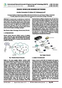
2. Disaster Management Scenario The new emergency response system we propose is based on the disaster management strategy followed for disasters like chemical explosion, fire in building etc. The on-site organization chief (OOC) designates the disaster site into several zones [2] (see Fig. 1). The hot zone, also referred to as the exclusion zone, is the area where contamination may occur. The warm zone is the area where the Contamination Reduction Corridor (CRC) is located. The cold zone area is chosen for forming the triage zone (TZ), the treatment zone (TTZ) and the transport zone (TRZ). Triaging is a method to classify the patients according to the severity of their injury and prioritize them for evacuation. There are four different classes of triaging:- Red: patients who require immediate attention, Yellow: patients who require delayed attention, Green: patients with light injuries, Blue: patients with no hopes of survival.
International Journal On Advances in Internet Technology, vol 2 no 1, year 2009, http://www.iariajournals.org/internet_technology/
69
information flow etc. AID-N mainly focuses on critical patient monitoring [4] at the disaster site. But in our emergency response system we have mainly focused on solving logistic problems which are critical at the disaster site.
3. Disaster Aid Network (DAN)
Fig. 1. Disaster Site Zones
2.1 Field study A disaster simulation drill was conducted by state fire department Bruchsal, Germany. The on-site organization chief (OOC) drew a map and accounted the details of the number of medical responders, transport vehicles, zones [3]. The manual mapping was time consuming, complex for updating real time changes and the resource estimation was hindered. With a resource limited response team, patients often wait for an extended period of time before transport. There is no continuous patient vital sign monitoring currently used [5]. The paper based triage is a bottle neck and makes the re-triaging difficult [6]. In addition, patients with minor injuries often depart the scene without notifying the response team, thus creating an organizational headache for OOC. At the San Diego disaster drill [4] conducted by UCSD/Calit2 (University of California San Diego), the simulation of a car bomb detonation that destroyed the taxi and sent plumes of charcoal-grey smoke containing lethal chemicals was undergone. The emergency officials found it complex to identify the high temperature zones that could harm the patients. The plumes or the colorless gases were heading in the direction of the victim holding area in the cold zones and caused respiratory hazards.
2.2 Related Works for Emergency Response Sensor Networks The Advanced Health and Disaster Aid Network (AID-N) from Johns Hopkins University, Applied Physics Laboratory develops technology-based solutions for time-critical patient monitoring, ambulance tracking, web portals for patient
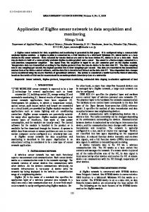
An emergency response system is proposed based on the DAN [1] to solve the problems mentioned in Section 2.1. The DAN architecture (see Figure 2) consists of hundreds of nodes distributed in a disaster site and wirelessly interconnected to form a mesh network. Several standard wireless technologies (ZigBee, WLAN, etc) are investigated and ZigBee is chosen as the wireless technology for DAN, since it’s a low power and a standard-based technology for interconnecting large number of nodes [7] [8]. The DAN ZigBee network uses the 2.4 GHz band which operates worldwide, with a maximum data rate of 250kbps [7]. ZigBee network can access up to 16 separate 5 MHz channels in the 2.4 GHz band, several of which do not overlap with US and European versions of IEEE 802.11 or Wi-Fi. It incorporates an IEEE 802.15.4 defined CSMA-CA protocol that reduces the probability of interfering with other users and automatic retransmission of data ensures robustness. Its self-forming feature enables the mesh network to be formed by itself thereby enabling the network to be easily scalable. Its self-healing mesh network architecture permits data to be passed from one node to another node via multiple paths. Its security toolbox ensures reliable and secure networks. The MAC layer uses the Advanced Encryption Standard (AES) as its core cryptographic algorithm and describes a variety of security suites that use the AES algorithm. These suites can protect the confidentiality, integrity and authenticity of MAC frames. There are three logical device types in ZigBee namely- the coordinators, routers, and end devices. A coordinator initializes a network, manages network nodes, and stores network node information. A Router node is always active and participates in the network by routing messages between paired nodes. The routing is based on the simplified Ad-hoc on demand Distance Vector (AODV) method. An end device is the low power consuming node as it is normally in sleep mode most of the time. It can take 15 ms (typical) to wake up from sleep mode [8].
International Journal On Advances in Internet Technology, vol 2 no 1, year 2009, http://www.iariajournals.org/internet_technology/
70
• • •
Scalability of the network Routing capability of nodes and effect on the number of routers in the network Impact of mobility of the nodes and the node heterogeneity
4.1 Related Works for ZigBee Simulation
Fig. 2. DAN Architecture DAN is a heterogeneous network [9] [10] formed with the following type of nodes: Patient node: Minimized electronic triage tag, localization support, ZigBee mote, vital and activity sensors, RFID tag. Emergency doctor node: PDA with GPS and ZigBee mote for patient monitoring and data recording Static anchor (router) nodes: ZigBee motes with known location coordinates, environmental sensors (ex: air temperature) that can be deployed at the site. Monitor station (coordinator): It is a collector node used by the EMC / OOC which supports data aggregation; visualization of inter-zone patient flow, transport capacity indication, patient location, triage information and patient vital signs [11]. At the beginning of the emergency response the OOC classifies the zones of the disaster site. The monitor station which is a portable device (notebook) gets online; the static anchor nodes (reference nodes for patient localization) are deployed manually covering the disaster area; the emergency doctor nodes [6] act as mobile anchor nodes; once a patient is found the doctor provides a wearable patient node. Each patient node (blind node) updates the monitor station with real time patient data.
4. ZigBee Simulation In order to find out the suitability of ZigBee for DAN-Architecture ZigBee mesh network simulations are done. The analysis of statistics like application traffic sent vs. application traffic received, end to end delay, and packet loss ratio is done for every simulation setup to investigate the following features:
In [17], Gianluigi Ferrari et al. analyze the influence of relaying nodes in ZigBee networks. He shows that the use of relaying nodes degrades ZigBee networks and that the use of acknowledgment messages highly increases the network performance. But the impact of relaying nodes only on a static ZigBee network is analysed and the effect of relaying nodes on static and mobile ZigBee networks is unknown. In [18] NiaChiang Liang et. al. investigate the influence of node heterogeneity on ZigBee networks. The behaviour of a ZigBee network with different percentage of end devices is analysed but the analysis is limited to a fixed number of nodes with a fixed range and a fixed transmission rate of 10 packets/sec. Furthermore the mobile nodes in this simulation move according to the random waypoint mobility model which is not realistic for our Disaster Management Scenario. In [19] LingJyh et. al. discuss about the influence of mobility in ZigBee networks. He shows that both the number of mobile nodes and the speed of the nodes severely affect the ZigBee networks. He also tells that the use of an end device as mobile receiver will degrade the network performance. But for investigating the effect of mobility, he uses random waypoint which is not realistic for our scenarios. Therefore we have developed our own self-defined trajectory based mobility models to investigate the effect of mobility if ZigBee is used for the DAN.
4.2 Simulator Several SOA simulators like NS2 [28], OPNET [20] are surveyed and OPNET is chosen for our simulation because OPNET allows simulation of complex networks and includes a ZigBee model library that implements the important features of the ZigBee standard [20]. OPNET supports the mobility models: random waypoint as well as self defined trajectories. The OPNET statistics for analysis are classified into two main groups: local statistics and global statistics. Local statistics describe the behavior of a particular node while the global statistics describe the behavior of the global network.
International Journal On Advances in Internet Technology, vol 2 no 1, year 2009, http://www.iariajournals.org/internet_technology/
71
4.3 Simulation Setup and Analysis In this section, we perform ZigBee simulations using OPNET simulator in static and mobile scenarios (since DAN has both static and mobile nodes) and analyze the results to find out ZigBee’s suitability for DAN. Before running simulations ZigBee’s stack parameters are configured according to the needs of our application. 4.3.1 ZigBee Stack Parameter Application layer: The packet size is set to 100 Bytes and the transmission rate is set to 1packet/20sec. In DAN, packet can be delivered either at a particular time interval or when an event occurs (ex: patient movement). MAC layer: Packet Acknowledgment is enabled. Acknowledgment wait duration is set to 864µsec. The number of retries is set to three. Network layer: The ‘network maximum depth’ is set to 5, ‘network maximum children’ is set to 20, ‘network maximum router’ is always less than or equal to the count of ‘network maximum children’ parameter.
Fig. 3: Application traffic sent vs. Application traffic received Figure 4 shows the packet loss ratio (in percentage) with increase of the number of nodes. The PLR increases linearly between 20 and 150 nodes after which it increases drastically. With more traffic the probability that a packet get lost is higher as the risk of collision through hidden nodes becomes higher.
4.3.2 Static Scenario Two static scenarios are developed: offline node scaling scenario and routers influence scenario. 4.3.2.1 Offline Node Scaling Scenario In this scenario the network area is set to 300m x 300m with the nodes randomly placed over the area. The transmission range of the nodes is fixed to 100 meters. All nodes transmit packets to a single collector node (coordinator) which only receives and doesn’t send any traffic. Several simulations are run by varying the total number of nodes (20, 50, 70, 100, 150 and 200). 50% of the total number of nodes acts as router. Figure 3 compares the application traffic sent (by all the nodes in the network) to the application traffic received (by the single collector node), when the number of nodes is varied from 20 to 200. It is seen that the network scales well up to 150 nodes. From 150 nodes to 200 nodes, the traffic loss is around 400bit/sec. The traffic loss is high due to the increase of network density which inturn increases the channel access attempts and thereby the retransmissions. After the three retransmission attempts, the packet is dropped.
Fig. 4: Packet Loss Ratio for offline node scaling scenario Figure 5 depicts the end-to-end delay (ETE) which is defined as the time elapsed, since a packet is sent by a sending node to a receiver node, and the reception of the Acknowledgment by the sending node. Similar to PLR the ETE also increases with the number of nodes. It increases slowly from 20 to 100 nodes, and then it increases exponentially. When the number of nodes increases, the number of attempt of the application traffic sent also increase. According to the channel access mechanism (CSMA-CA), the nodes listen to the medium before they send. If the medium is busy, they wait for a randomly chosen time and then try again. With more nodes attempting to access the channel, the probability that the channel is busy becomes higher. Also with larger number of nodes, the channel is busier and consequently, the number of retries is increased.
International Journal On Advances in Internet Technology, vol 2 no 1, year 2009, http://www.iariajournals.org/internet_technology/
72
increases the traffic considerably in the network. When a node needs to send data, it broadcasts a route request message (RREQ). All the neighbouring routers receive this message and broadcast it until the message reaches the destination. The receiver receives the RREQ message from all it surrounding routers and sends back a route reply (RREP) message through the shortest route (in terms of number of hops). So using more routers in a static scenario does not improve the performance.
Fig.5: End to End Delay for offline node scaling scenario 4.3.2.2 Router Influence Scenario In this scenario the impact of routers on a static network is analyzed. The network area is set to 300m x 300m, the node transmission range is set to 100m, fixed total number of nodes is set to 100. The percentage of routers in the network is varied from 20 to 100 % and the effect of routers is analysed. In Fig. 6, both the application traffic sent (red line) and the application traffic received are almost the same as the number of routers are increased from 20 to 100%. This shows that the number of routers has no impact on the application traffic received.
Fig. 6: Application traffic sent vs. Application traffic received - Router Influence scenario In Fig. 7, the PLR remains stable between 20% and 30% after which it increases linearly. Even though the application traffic sent and received are almost the same (see Fig. 6) the PLR is very high. Although we have the same number of nodes, having more routers
Fig. 7: PLR – Router Influence scenario In Fig. 8 the ETE increases with increase in router percentage. Thus it can be concluded that the number of router has no impact on the application traffic received. However, the PLR and the ETE increases as the number of routers increases. Whether these values of ETE and PLR are critical depends on the application.
Fig. 8: ETE - Router Influence scenario
4.3.3 Mobile Scenarios Two mobile scenarios are defined: random trajectory mobility model and disaster management mobility
International Journal On Advances in Internet Technology, vol 2 no 1, year 2009, http://www.iariajournals.org/internet_technology/
73
model. The random trajectory model simulates a general mobile scenario where the movement pattern of the nodes is defined by self-defined trajectories, unlike the ‘random waypoint mobility model’. The Disaster Management Model represents realistic movement pattern of the nodes during emergency response.
receive the acknowledgment message and the packet is considered as lost. It can be seen from Fig. 10 that mobility severely affects ZigBee networks.
4.3.3.1 Random Trajectory Mobility Model In the random trajectory mobility model, we defined our own trajectories for all the nodes. Each node moves with predefined trajectories throughout the network area. The network area is set to 300m x 300m, simulation duration is set to 300 sec, and the node transmission range is 100m. The total number of end devices is set to 70. Furthermore 10 static routers are distributed to cover the network area. Fig.9 shows the random trajectory mobility model snapshots at the beginning and at the end of the simulation. The nodes are set in groups at the beginning of simulation. The white arrows define the trajectories of the nodes. As the simulation progresses the nodes move to predefined positions within the network area according to their trajectories.
Fig. 10: Application traffic sent vs. application traffic received for Random Trajectory Model 4.3.3.2 Disaster Management Mobility Model In this mobility model the realistic movement pattern of the nodes at the disaster site are setup based on the emergency response process followed (see Section 2). This mobility model uses online node scaling ie. the nodes join the network with increase of time and a few nodes to leave the network toward the end of the simulation. Two models are simulated: 50%-router-model and 100 %-router-model. 50%-Router-Model
Fig. 9: OPNET network panel at the beginning and end of simulation Figure 10 shows the application traffic sent compared with the application traffic received in the random trajectory mobility model. At the simulation start time, the application traffic sent and received are same. But after about 20 seconds the application traffic lost increases and at the end of the simulation only 1050 bit/sec is received of the 2500 bit/sec sent. In this scenario, only few nodes transmit packets at the simulation start time and as time progresses more nodes transmit and begin to move throughout the network area. The application traffic lost is high because the end devices send packets to their destination through a parent router and in most cases it could be that the node (after sending its packet) moves out of the range of its parent router thereby failing to
In this model 50 % of the total nodes are set as routers. The network area is set to 500m x 500m with a total of 100 nodes, of which 50 nodes are end devices (all patient nodes in DAN are set as end devices). The other 50 nodes are set as routers (15 routers are static representing the static reference nodes and 35 routers are mobile representing the emergency doctors in DAN). Furthermore, the node transmission range is set to 100m and the simulation duration is 2000sec. In the disaster management mobility model, the network area is divided into four zones: the disaster zone (DZ), the triage zone (TZ), the treatment zone (TTZ), and the transport zone (TRZ). At the beginning of the simulation, 15 static routers are distributed over the area, to make sure that the whole network area is covered. At the simulation start all patient nodes are located at the danger zone and the emergency doctor nodes are progressively entering the network. Some emergency doctor nodes move to the danger zone.
International Journal On Advances in Internet Technology, vol 2 no 1, year 2009, http://www.iariajournals.org/internet_technology/
74
Some doctors move directly to the triage zone and start with the triaging as soon as the first patients arrives the triage zone. The rest of the doctor nodes are moved to the treatment zone and then to the transport zone. By this configuration, it’s made sure that there will always be a few doctor nodes in each zone at any time unit. Fig. 11 shows a snapshot of the network at the beginning of the simulation. The four zones are marked by rectangles and the white lines define the trajectories of the nodes. As the trajectories show, most of the nodes have the following flow: DZ Æ TZ Æ TTZ Æ TRZ. But there are some exceptions, especially for emergency doctors. Also some patient nodes leave the network after they have been transported to the TZ or to the TTZ. The red, green, yellow and blue colour nodes represent the patients. The nodes with a cross represent the emergency doctors. A patient is assisted by at least one doctor from the DZ to the TZ after which the doctor moves back to the DZ. The patients are triaged by the doctors who are already present in the TZ. According to their triage class priority (red first, followed by yellow and green) the patient are shifted to the TTZ and finally to the TRZ.
Fig. 12: 50%-Router-Model snapshot after 1000 sec of simulation In Fig.13, at the beginning of the simulation not all nodes are sending and not all nodes are already moving thus the application traffic lost is less. At 500 seconds all the nodes have joined the network. Since all the patient nodes are sending and the network is highly mobile the application traffic lost is high. After 1650s no more patient nodes are present and the network contains only few doctor nodes, static anchor nodes and so almost all the application traffic sent is received. It can be seen that the mobility affects ZigBee network, but in comparison with the results of random trajectory mobility model the performance (in term of application traffic received) is better for the 50%-Router Model which can be due to the varying mobility patterns.
Fig. 11: 50%-Router-Model snapshot at the start of simulation Fig. 12 shows the state of the network after 1000 sec. All mobile nodes have already moved from DZ to TZ and from TZ to TTZ. There are also some patient nodes in TRZ and some have already been transported (evacuated) to the hospital. At the end of the simulation, the site is almost empty and there are no more patient nodes. There are only doctor nodes and static reference nodes in the network.
Fig. 13: Application traffic sent vs. application traffic received for the 50%-Router-Model
International Journal On Advances in Internet Technology, vol 2 no 1, year 2009, http://www.iariajournals.org/internet_technology/
75
100%-Router-Model
4.3.4 Results
The simulation setup for this model remains the same as that of 50%-Router-model except that all patient nodes are now routers (i.e 100% routers in the network).
Scalability: In a static scenario the network scales well, as far as the density of the network is concerned ie. the network scales well up to 150 nodes in a 300m x 300m area. When the number of nodes is increased above 150 the application traffic loss is high (about 400bit/sec). In a mobile scenario, the network does not scale as well as in the static scenario due to the high PLR.
In Fig. 14, the application traffic received for the 50%-Router-Model and 100%-Router-Model are compared to find the impact of routers in a mobile disaster management scenario. The application traffic received is better when all the patient nodes are set as routers because routers are more robust than end devices against the influence of mobility.
Influence of routers in the network: In a static scenario using more routers doesn’t improve the network, rather it degrades the performance (PLR, ETE). But in mobile scenario, the use of more routers considerably improves the performance of the network. So in a static network only the number of routers required to cover the network area, can be used. In a mobile network it may be suitable to use as many routers as possible. Mobility: The performance of ZigBee network is affected when the nodes are mobile, especially when the mobile node density is high. However, the performance could be improved if the number of routing capable devices is increased.
Fig. 14: Comparison of application traffic received for 50%-Router-model and 100%Router-model In Fig. 15, the PLR when patient nodes act as end devices and the PLR when patient nodes act as routers are shown. With more routers, fewer packets are lost.
ZigBee is basically suitable for the DAN, even though more detailed investigations are required. As part of future work the influence of node density and effect of more than one collector node will be investigated.
5. ZigBee Mesh Network In order to perform the RSSI based localization analysis and to setup an air temperature monitoring demonstrator we have developed a 20 node ZigBee mesh network.
5.1 ZigBee-ready temperature Sensor Node
Fig. 15: Comparisof PLR for 50%-Routermodel and 100%-Router-model The mobile scenario performs well in presence of routers, which is in contrast to static scenario. Routers dispose of functionalities that make them robust against mobility effects.
The temperature sensor node [21] is designed with a power supply, Texas Instruments (TI) CC2431 System on Chip (SOC) and chip antenna. The CC2431 (see [12], [13]) consists of the location engine, RF transceiver, an enhanced 8051 MCU, and a temperature sensor. The current consumption of this sensor node (see Figure 16) is shown in Table 1. The ZigBee router is always active, leading to higher current consumption. In the communication deactivated state (8051 core active, RF transceiver off), the end device is in sleep mode leading to lower current consumption. In DAN
International Journal On Advances in Internet Technology, vol 2 no 1, year 2009, http://www.iariajournals.org/internet_technology/
76
the nodes may require a battery lifetime of around 5 hours to one week. The current consumption results show that the sensor node can be used as the patient nodes or doctor’s node or routers and last at least for few days.
Fig. 16. ZigBee-ready Temperature Sensor Node Table 1. Current Consumption of Temperature Sensor Node ZigBee Sensor Node (supply voltage = 3.0 V) Data communication activated Data communication deactivated
Router 35.8 mA
End Device 27.8mA
-
20.4 mA
6 Patient Localization during Emergency Response A patient localization solution has to be developed, that provides real time patient’s location to the medical / organizational officers and in tandem with the emergency response system facilitates efficient logistics at the disaster site. Each patient node (blind node) runs a localization algorithm and updates the monitor station with its current location information. The requirements [22] for patient tracking that DAN must comply with are: handle the different environments (both outdoor and indoor); use little or no special infrastructure (static anchor nodes) due to lack of deployment time at the site; track 30-500 patient nodes moving with varying speed (0 to 3 m/s); attain an accuracy of 5 to 10 m with a max latency per node of 5 seconds; be scalable and robust. The main challenge here is to handle the varying mobility and different environment with adverse RF conditions and also use minimum or no infrastructure.
6.1 Related Work for Patient Localization Localization systems like Active Badge [23], Cricket [24], RADAR [25] required a lot of infrastructure and GPS [26] is not suitable for Indoor. RFID based solutions like SpotON [27] are not suitable for us since
they demand high anchor node density, works in short range and needs a fixed infrastructure.
6.2 Analysis of a Received Signal Strength Indicator (RSSI) based Localization system An analysis of the CC2431 hardware based location solution is undergone to find its suitability to the DAN. The CC2431 Location Engine [12], [13] hardware from Texas Instruments (TI) implements a distributed computation algorithm that uses RSSI values from reference nodes whose coordinates are known to calculate the location of the blind nodes whose coordinates are to be determined. Performing location calculations at the node level reduces network traffic and communication delays otherwise present in centralized computation approach. 6.2.1 RSSI based Localization- Functionality The basis of this radio-based positioning solution is the relation between the distance from the transmitter and the received signal strength (see equation 1) considering the assumption that the propagation of the signal is approximately isotropic [14].
RSSI = −(10nlog10 d + A).
(1)
The parameters A and N determine the exactness of the blind node location. A is an empirical parameter determined by measuring the absolute RSSI value in dbm of an omni-directional signal at a distance of one meter from the transmitting unit. The parameter N is defined as the path loss exponent and describes the rate at which the signal strength decreases with increasing distance from the transmitter [14]. The positioning of blind node is done by averaging at least three and a maximum of eight references nodes. Localization takes place in two steps, which are repeated in cycles. The first step is the Burst-phase, in which the blind node broadcast a sequence of packages, requesting the reference nodes for their position and the averaged received signal strength of the packets sent to them. In the second step the eight best received references will be sorted according to their signal strength and handed over along with the parameters A and N values to the blind node (localization hardware) which solely calculates its location [14].
International Journal On Advances in Internet Technology, vol 2 no 1, year 2009, http://www.iariajournals.org/internet_technology/
77
6.2.2 Analysis A 120 x 120 meter indoor area is covered by rectangular grid of sixteen reference nodes each separated by 40 meters. ZigBee ready sensor nodes are used as reference and blind nodes. The coordinator is a ZigBee hardware dongle enabled laptop running Location Graphical User interface (GUI) software to display the positions of nodes in the site map. The location (x,y) of the reference nodes are manually configured via Z-location engine a display and control software [14]. The value of A is measured as 49 and the value of N is selected as 3.875 from the vendor specification, based on the empirical measurement that best fits the environment. Five blind nodes are moved within this grid to 10 different positions (center of grid, corners) at an interval of 20 seconds and the corresponding position coordinates are measured via the Location GUI. The actual location and the measured location of the blind nodes are compared. The average deviation of the measured values from the actual values, for 10 different readings is calculated for each blind node and an accuracy of 2 meters is obtained. The time (burst phase plus computation phase) for every blind node to calculate its location is measured as 2 seconds. It is noticed that as people/objects moved in the indoor area the blind node location estimation was varying and unstable. The analysis of the CC2431 localization solution reveals that the blind node location estimation is unstable and needs large number of reference nodes for considerable performance. So this system is also not suitable [21] for our scenario. Therefore we are currently developing a new localization solution for our scenario.
7
Air Temperature Monitoring
In DAN, the ZigBee mesh network consists of sensor nodes to sense local weather conditions like air temperature, wind speed and wind direction. The wind speed and wind direction information can enable the emergency responders to identify zones filled with colorless toxic gases. This can allow the responders to quickly shift the patients away from these danger zones and reduce respiratory hazards. In this paper we have focused on air temperature monitoring only. The air temperature at the different zones of the disaster site varies throughout the disaster management process. We have implemented an air temperature monitoring mesh network that provides real time
temperature information at the disaster site. These data are collected by the monitor station which runs the visualization software. The visualization software runs the temperature zone algorithm and displays various temperature zones at the disaster site.
7.1
Temperature Zone Algorithm
The temperature zone algorithm [21] is a dynamically responding mechanism [16] based on localized temperature events. The functionality of this algorithm is to estimate and display the various temperature zones present at a disaster site. The algorithm is implemented in Python using NumPy (Numerical Python) for matrix processing and wxWidgets / wxPython for the graphical user interface. The inputs to this algorithm are: • The location coordinates of the temperature sensor nodes • The measured temperature values from the sensor nodes The output from this algorithm is: • The estimated temperature zone mapping • The current algorithm implementation detects only two zones: danger zone (30°C to 50°C), normal zone (20°C to 29°C). 7.1.1 Functionality The functional block diagram of temperature zone algorithm is as shown in fig.17.
Fig. 17. Functional Block Diagram of Temperature Zone Algorithm Temperature Zone Mapper The location of the temperature sensors and their corresponding temperature readings are given as input into the temperature zone mapper. For every location coordinate received, the temperature zone mapper uses the corresponding temperature reading to calculate a cosine probability distribution of the temperature centered at the given location coordinate and weighted with the temperature value for that location coordinate. For example, assuming the algorithm gets a temperature value of 30°C at a location coordinate (20,20) then the temperature zone mapper plots a probability distribution function (as shown in fig. 18)
International Journal On Advances in Internet Technology, vol 2 no 1, year 2009, http://www.iariajournals.org/internet_technology/
78
centered at (20,20). As the distance increases away from the location (20, 20) the probability for the temperature to be 30°C is less.
Display Temperature zones are displayed by assigning a color to each location of the output of the grid based on temperature range. Danger zone is displayed in red and normal zone is displayed in blue. The resulting color of each output is calculated by multiplying the output of the grid with the assigned color for its corresponding temperature range.
7.2 Demonstrator Fig. 18 Temperature Probability Vector Grid block The Grid block is a three dimensional representation of the display block where time is the third dimension. It generates a three dimensional
r T ( x, y,t ) vector as output for every location coordinate given as input and stores this value in the r (x, y,t ) in the grid is calculated T grid. The value of by adding the output of the temperature zone mapper to the decayed previous grid value at that location (see equation 2). The values of the grid are instantaneously calculated and updated at each time step for all location coordinate inputs. This enables the tracking of temperature variation at a particular location. The grid functionality is mathematically shown below. r T ( x, y, t ) =
r
∑ T (x, y ) ⋅ decay (t − t ) ev
ev
(2)
For efficient implementation, a decreasing exponential function is used for delay. decay(x) = a x ,0 < a < 1
r By substituting the decay function in T (x, y, t) and expanding the summation, we get t − t ev r r r t − t ev n 1 T (x, y, t) = T ev (x, y) ⋅ a + ... + T ev (x, y) ⋅ a n 1
(3)
A 20 node ZigBee mesh network is set up covering an indoor area of 120 x 120 meters. Each temperature sensor node (see Section 5.1) was displaced by around 40 meters to form a rectangular grid of static routers and end devices. The location coordinates of the nodes were manually configured. The temperature values with its corresponding location coordinates are periodically transmitted to the monitor station running the visualization software. This visualization software consists of a display and summary panel. The display panel shows the various temperature zones in different colors over a map of the site where the mesh network was deployed. The summary panel provides the temperature values of the nodes at its corresponding location textually. When the mesh network was started the nodes sensed a room temperature value which falls under the normal zone and so the display panel indicates the entire deployment site in blue color (see figure 19-a). But as the mesh network was running we gradually heated the nodes at the bottom half of the grid above 30°C using the heat gun. We were able to see in real time, the bottom half of the deployment sites map (in the display panel) changing to red color indicated a danger zone (see figure 19-b).
(4) Extraction of a summands between 1 and n − 1 yields t −1−tev t −tev t −1−tev r r r r n−1 ⎞ 1 T(x,y,t)= a⎛⎜Tev (x,y)⋅ a +...+Tev (x,y)⋅ a ⎟+Tevn (x,y)⋅ a n − n 1 1 ⎝ ⎠
r By substitution of T (x, y, t − 1 ) for events from 1 to n − 1 , we get t − t ev r r r n T (x, y, t) = a ⋅ T (x, y, t − 1 ) + T ev (x, y) ⋅ a n
(5)
(6)
t = t ev
n , this is further simplified to When r r r T (x, y, t) = a ⋅ T (x, y, t − 1 ) + T ev (x, y)
n
(7)
Fig.19 a) Normal Zone Visualization
International Journal On Advances in Internet Technology, vol 2 no 1, year 2009, http://www.iariajournals.org/internet_technology/
79
temperature sensor node indicate that they can have a lifetime of at least few days as patient wearable nodes or temperature sensor nodes in DAN. The analysis of RSSI based localization solution shows that it’s not suitable to DAN due to its need for large infrastructure and unstable blind node location. So a new localization solution for DAN will have to be developed as future work. The result of the temperature zone algorithm shows its computational efficiency and its effectiveness in alerting the responders about danger zones. The patients can therefore be quickly evacuated from the disaster site. Further expansion of the system and its testing with large scale networks is part of the future work. Fig.19 b) Danger Zone Visualization
7.3 Computation analysis of Temperature zone algorithm The temperature zone algorithm was only evaluated using a mesh network of 20 nodes. In order to find the computation efficiency of this algorithm in large scale mesh network the algorithm is analyzed by giving an event log file containing the events (temperature values at different location coordinates) as input (see fig. 20).
Fig. 20 Analysis Model for Temperature Zone Algorithm 1006 randomly generated events were fed as input to the algorithm at once, to estimate the performance of the temperature zone algorithm. The analysis was run on an Intel Pentium 1.6GHz processor and took 484.65 seconds of CPU time (396.7s user and 33.7s system) to complete its run. From this, we can infer that on a comparable or better processor, the temperature zone algorithm will be able to process 2 or more events per second.
8
Conclusion
A new emergency response system based on the location aware DAN is proposed for assisting the ER’s at the disaster site. The ZigBee simulation results for scalability, mobility and number of routers show that ZigBee is basically suitable for DAN even though detailed investigations will have to be done. The current consumption results of ZigBee-ready
9 References 1 Chandra-Sekaran, A. and Nwokafor, A. and Johansson, P. and Mueller-Glaser, K. D., and Krueger, I. ZigBee Sensor Network for Patient Localization and Air Temperature Monitoring During Emergency Response to Crisis. The Second International Conference on Sensor Technologies and Applications, SENSORCOM 2008, France. 2 Hazardous material management http://www.epcra.state.mn.us/hazmat_info/scene_safety.html 3 “Gesetz über den Rettungsdienst sowie die Notfallrettung und den Krankentransport durch Unternehmer (Rettungsgesetz NRW - RettG NRW) Vom 24. November 1992”- Emergency Response Law in the German state NRW. 4 San Diego Disaster Drill http://www.calit2.net/newsroom/article.php?id=745 5 Gao, T. and Greenspace, D. and Welsh, M. and Radford, R. J. and Alm, A. Vital sign monitoring and patient tracking over a wireless network. Johns Hopkins University, Applied Physics Laboratory. 6 Gao, T. and White, D. A next generation electronic triage to aid mass casualty emergency medical response. Johns Hopkins University, Applied Physics Laboratory. 7 “ZigBee Specification 2006” ZigBee Alliance, Tech. Rep.Document 053474r13, 2006. 8 ZigBee Alliance website http://www.zigbee.org/ 9 Hac, A. Wireless Sensor Network Designs. University of Hawaii at Manoa, Honolula, USA. 10 Zhao, F., and Guibas, L. Wireless sensor networks, an Information processing approach. 11 Chandra-Sekaran, A. and Mueller Glaser, K. D. and Stork, W. and Picioroaga, F. and Brinkschulte, U. Towards a self-organizing wireless hospital area network. World Congress in Medical Physics and Bio-Medical Engineering, Seoul, South Korea, 2006. 12 Texas Instruments CC2431 - System-on-Chip for 2.4 GHz ZigBee/ IEEE 802.15.4 with Location Engine: Data sheet 13 Texas Instruments CC2430 - System-on-Chip for 2.4 GHz ZigBee/ IEEE 802.15.4: Data sheet 14. Texas Instruments CC2431 Location Engine: Application Note AN042
International Journal On Advances in Internet Technology, vol 2 no 1, year 2009, http://www.iariajournals.org/internet_technology/
80
15 “NRW, Behandlungsplatz-bereitschaft: Konzept BHP-B 50 NRW. Innenministerium des Landes NordrheinWestfalen, April 2006”-NRW state treatment zone concept BHP-B 50 NRW. 16 Tatomir, B. and Rothkrantz, L. Ant based mechanism for crisis response coordination, Proceedings of Ant Colony Optimization and Swarm Intelligence, ANTS 2006 17 Ferrari, G. and Medagliani, P. and Martaló, M. Performance analysis of ZigBee wireless sensor networks with relaying. Wireless Ad-hoc and Sensor Networks (WASN) Laboratory, Department of Information Engineering University of Parma, Parma, Italy. 18 Nia-Chiang Liang, Ping-Chieh Chen, Tony Sun, Guang Yang, Ling-Jyh Chen, and Mario Gerla, Impact of Node Heterogeneity in ZigBee Mesh Network Routing. 2006 IEEE International Conference on Systems, Man and Cybernetics, October 8-11 2006, Taipei, Taiwan. 19 Ling-Jyh, Tony Sun, Nia-Chiang Liang, An Evaluation Study of Mobility Support in ZigBee Networks. Institute of Information Science, Academica Sinica. 20 OPNET online documentation. http://www.opnet.com/, 21 Ranjan, G. and Kumar, A. and Rammurthy, G. and Srinivas, M. B. A natural disaster management system based on location aware distributed sensor networks. MASS2005, 0-7803-944-6/05/. 22 Lechtleutner, A. Disaster Management process Investigation- University of Applied Sciences, Rescue Engineering Department. 23 Want, R. et al., The active badge location system, ACM Trans. Inf. Syst., pages 91-102, 1992 24 Priyantha, N. B. and Chakraborty, A. and Balakrishnan, H. The Cricket Location Support System, ACM Press, Proceedings of the 6th annual international conference on Mobile computing and networking (MobiCom’00). pages 3243, 2000 25 Bahl, P. and Padmanabhan, V. RADAR: An inbuilding RF based user location and tracking system, Proceedings of IEEE Infocom. vol. 2, pages 775-784, 2000 26 Global Positioning System http://www.gps.gov/ 27 Hightower, J. and Borriello, G. SpotON: An Indoor 3D Location Sensing Technology Based on RF Signal Strength 28 ns-2 Simulator http://www.isi.edu/nsnam/ns/