A distributed scheduling methodology for a two

A distributed scheduling methodology for a two-machine flowshop using cooperative-interaction via multiple coupling-agents

In-Jae Jeong and V. Jorge Leon Texas A&M University College Station, Texas

(Manuscript Revised May 9, 2002) Under Review in Journal of Manufacturing Systems

Abstract This paper presents a distributed scheduling methodology for a two-machine flowshop problem. It is assumed that the decision authorities and information are distributed in multiple sub-production systems that must share two machines in order to satisfy their demands.

The associated scheduling problems are modeled using 0/1 integer

formulations, and the problem is solved using Lagrangian relaxation techniques modified to work in an environment where very limited information sharing is allowed. Specifically, no global upper-bound is known, no single decision entity has complete view of all the constraints that couple the participating sub-production systems, and there is no disclosure of local objectives and constraints. The main objective of the proposed algorithm is to find a compromise state where all coupling constraints and local constraints are satisfied, and the total sum of weighted completion time of jobs is minimized. The proposed methodology showed promising experimental results when compared to the traditional Lagrangian Relaxation with subgradient method. Keywords: Machine Scheduling, Distributed Production System, Distributed Decision Making, Lagrangian relaxation, decomposition methods

1

Introduction It is well known that scheduling systems rapidly become complicated, information intensive, and impractical when they are based on centralized and monolithic models of the system. Due to recent advances in Internet and network technologies, distributed scheduling offers a viable alternative to explicitly account for the distribution of decision authorities in an organization and model their local autonomy.

A main issue in

distributed scheduling is to investigate how different interacting organizations in a manufacturing system can cooperate to construct a detailed schedule which achieves optimal or close-to-optimal system-wide performance. In order to coordinate efforts, individual organizations must be able to acquire the information about the state of the system and communicate the local information to the rest of the system.

The

methodology in this paper is particularly suitable for situation where complete information about the entire system is not available to a single decision maker. Such a situation can arise due to organizational structures and information privacy policies. This paper presents a distributed scheduling methodology that allows for less information sharing than previous decomposition-based methodologies. Lagrangian Relaxation with subgradient method has been widely used for distributed job shop scheduling (Ovacik1; Roundy et al.2; Luh and Hoitomt3; Gou et al.4; Kutanoglu and Wu5). Lagrangian Relaxation has originated as a decomposition method to solve centralized problems that are linked by coupling constraints of special characteristics. Lagrangian Relaxation, as other mathematical decomposition methods, has some limitations for its application in distributed organization mainly because one master problem must have access to detailed information contained in every coupling constraint. Also, the master problem requires an explicit global objective function (i.e., a global upper-bound) that is assumed not available in this paper. Agent-based scheduling is common in the artificial intelligence (AI) literature. Constraint Heuristic Search (CHS) has been applied in multi-agent environments where cooperative agents perform scheduling tasks with job-based perspective or resourcebased perspective views (Fox and Smith6; Smith et al.7, 8; Sycara et al.9; Zweben and Fox10). CHS fits well with the AI models and provides a meaningful framework of a distributed system composed of job-based and resource-based agents. However, CHS

2

can hardly be incorporated with an optimization process since the objective of CHS is to find only a feasible schedule that satisfies various constraints and rules11. Asynchronous Teams, or A-Teams, is another AI methodology for distributed environments (Talukdar et al.12). A-Teams are partially composed by agents, associated with problem-solving methods, that work together to solve a common problem by sharing their solutions via common memories. To operate effectively, A-Team agents typically have a complete view of the problem and must share their complete solutions with others. In contrast, in the scenarios of interest for this paper, no decision entity has complete information about the problem, and their solutions are only partial solutions to the overall problem. The approach in this paper uses Cooperative Interaction via Coupling-agents (CICA, Jeong and Leon13). CICA provides a general mathematical methodology for decision making in organizationally distributed systems. In CICA, interactions are established among cooperating organizations and coupling-agents. A coupling-agent is an artificial entity that is associated with a subset of coupling constraints.

CICA has been

successfully applied to problems with different structures; namely, non-linear continuous optimization13, linear programming14, and 0/1 integer programs15. The latter application presents an implementation in the context of a single-machine distributed scheduling problem with precedence constraints. Distinctively, this paper considers the case where the coupling constraints are divided into two sets, each one assigned to independent decision entities.

This characteristic distinguishes the proposed methodology from

existing mathematical decomposition methods where a single entity (i.e. a master problem) must have complete responsibility for all of the coupling constraints.

Two-shared-machine problem The decision problems under consideration are formulated as 0/1 integer programs using the notation proposed by Pritsker et al.16 and Kutanoglu and Wu5. In the two-shared-machine problem, there are m sub-production systems. For each sub-production system i, ni jobs need to be processed on two machines sequentially. The total number of jobs is

m

∑n

i

= N . The local objective of each sub-production system is to

i =1

minimize the sum of the weighted completion time of its jobs. The local constraints of

3

the sub-production system are the precedence constraint for each job to ensure the machines are visited in the required order, and the machine capacity constraints associated with its jobs. The global goal of the system is to minimize the total sum of the local objective functions.

The two-machine flowshop problem to minimize total

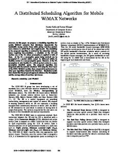
weighted completion time is NP-hard11. Figure 1 illustrates the disjunctive representation of a two-machine flowshop scheduling problem with two sub-production systems.

Sub-production system 1 is

responsible for the production of jobs J1 and J2, and sub-production system 2 is responsible for jobs J3 and J4. The first and the last node of each sub-production system are artificial nodes representing the starting and the end nodes. All other nodes represent the operations of jobs and conjunctive arcs (solid arrows) describe the precedence relationship between operations. Ojk represents the kth operation of job j where k = 1,2. Disjunctive arcs (dashed arrows) connect operations competing for the same machine. Sub-production system 1 controls the starting time of O11, O12, O21 and O22 while satisfying the precedence constraints between O11 → O12 and between O21 → O22. Similarly, sub-production 2 controls the starting time of O31, O32, O41 and O42 while satisfying the precedence constraints between O31 → O32 and between O41 → O42. Due to this partial information sharing, sub-production systems’ solutions may violate machine conflict constraints on machine 1 and machine 2 since they do not know about other jobs scheduled on the shared-machines. Meanwhile, an artificial “coupling-agent” associated with shared-machine 1 must prescribe the starting times of O11, O21, O31 and O41, and a second coupling-agent associated with shared-machine 2 must prescribe the starting times of O12, O22, O32 and O42. The coupling-agent’s solution satisfies machine conflict constraints since each machine maintains complete information of machine conflict constraints. However, due to partial information sharing, the coupling-agents’ solutions may violate the precedence constraints because they are assumed private to each sub-production system. As it can be seen from the example, an important characteristic of the distributed scheduling problem under consideration is that no single sub-production or couplingagent has complete view or control of the overall system. This characteristic makes it impossible to solve the associated scheduling problem using a centralized approach. The

4

problem is to allocate operations of jobs to time slots on machines in order to achieve the global goal by the interaction of sub-production systems and shared-machines with a minimum revelation of local information. Global solutions are achieved by carefully exchanging local information among sub-production systems and the two couplingagents during this interaction.

O11

O12

Sub-production system 1

O22

O21 O32

O31 O41

Shared-machine 1

Sub-production system 2

O42

Shared-machine 2

Figure 1. Disjunctive graph representation of the two-shared-machine problem First, let’s introduce necessary notation to formulate the problem mathematically. T: the production horizon on machine 1 and 2. 1, if operation k of job j has started by time t. x jkt =   t = 1,.., T, k = 1, 2 0, otherwise. 

Ui: a set of jobs that belong to sub-production system i. sjk =

T

∑ (1 − x

jkt )

: starting time of operation k of job j.

t =1

pjk: processing time of job j on machine k, k = 1, 2. Cj = s j 2 + p j 2 =

T

∑ (1 − x

j 2t ) +

p j2 :

completion time of job j.

t =1

wj: weight for unit completion time of job j. T must be large enough to process all jobs. Let T =

N

∑(p

j1

+ p j 2 ) . Also, the same index

j =1

k is used for an operation and a machine since for a flowshop the first operation is

5

processed on the first machine and the second operation is processed on the second machine. Figure 2 shows the decision structure and information flows of the proposed CICA model for a two-machine flowshop problem. Details are described in the following sections.

Shared-machine 1 (MP1) −1 n−1 n−1 sny11 , µ11 , π11

Shared-machine 2 (MP2)

−1 n−1 n−1 , µm1 , πm1 snym1

−1 n−1 n−1 snyi1 , µi1 , πi1

−1 n−1 n−1 snx11 , α11 , β11 sn−1 ,αn−1 , βn−1 x12 12 12

Sub-production system 1 (SP1)

Sub-production system i (SPi)

Sub-production system m (SPm)

Figure 2. CICA model for a two-machine flowshop problem Sub-production system problem (SPi) Let s nyjk−1 be the starting time of operation k of job j prescribed by the shared-machine k after (n-1)th iteration. For clarity, y is used in association with shared-machines, while x is used in association with sub-production systems. For instance, in order to differentiate a solution prescribed by the shared-machine and the ones for the sub-production systems, y njkt is introduced instead of x njkt to denote that the solution is associated with shared-

machine k.

µ njk−1 and π njk−1 are the Earliness/Tardiness (E/T) weights by starting the

operation k of job j one unit early/late from s nyjk−1 . These weights capture the effects of

6

local decisions on the overall system. Their determination and updating are fundamental for the proposed methodology and are described later. Given, s nyjk−1 , µ njk−1 and π njk−1 , the weighted completion time problem of sub-production system i at iteration n is formulated as follows:   T Min wj (1 − x nj 2t ) + p j 2  +   j∈U i   t =1

∑

(SPi): s.t.

2

∑

s nyjk−1   T  n −1 n n −1 n  µ x π ( 1 x ) + − jkt jk jkt   jk  t =1 j∈U i  t = s nyjk−1 +1  

∑∑ k =1

∑

x njkt +1 ≥ x njkt ∀j ∈ U i , k = 1,2, t = 1,..., T − 1 T − p jk +1

∑x

n jkt

≥ 1 ∀j ∈ U i , k = 1,2

∑

(1) (2) (3)

t =1

x nj1t − p j1 ≥ x nj 2t ∀j ∈ U i , ∀t

(4)

∑ (x

(5)

j∈U i

n jkt

− x njkt − p jk ) ≤ 1 ∀t, k = 1, 2

x njkt = {0,1}

Where

s nyjk−1

∑ t =1

∀j ∈ U i , ∀t , k . T

x njkt is the earliness and

∑ (1 − x

n jkt )

is the tardiness of job j with due date s nyjk−1 .

t = s nyjk−1 +1

The objective (1) of sub-production system i at iteration n is to find a compromise T

between the local optimal solution,

∑ (1 − x t =1

s nyjk−1 .

n jkt

) = s njkt , and the shared-machine’s solution,

Constraint (2) implies that once started, an operation remains started in all

subsequent time periods. Constraint (3) forces each operation to be finished within the production horizon by guaranteeing that the operation k of job j starts earlier than T − p jk + 1 .

Constraint 4 enforces the precedence constraint of a job between the first

operation on machine 1 and the second operation on machine 2. Constraint (5) represents the machine conflict constraint and ensures that at most one operation can be processed on the machine in the same time period. If complete information about machine conflict constraints were made available by the shared-machine, then sub-production system i could incorporate machine conflict constraints in its own local objective function as follows:

7

Min

2   T wj (1 − x j 2t ) + p j 2  −   j∈U i  k =1  t =1

∑

∑∑

∑

t

 θ kt 1 −  

 ( x jkt − x jkt − p )  . j  j∈U i 

∑

(6)

Where θ kt is the positive Lagrangian multiplier of the machine conflict constraint at the time t of machine k.

However, in this distributed environment, passing complete

information about machine conflict constraints is not allowed because it is private information of the shared-machine.

Instead the shared-machine passes only partial

information about the machine conflict constraint through an information vector which is composed of the shared-machine’s solution and E/T weights, or s nyjk−1 , µ njk−1 and π njk−1 , ∀j ∈ U i , respectively.

The solution of the shared-machine satisfies the machine conflict constraints but it may violate the precedence constraints of jobs since they are not known to the sharedmachine. The E/T weights reflect the marginal penalty of violating machine conflict constraints at the current shared-machine’s solution. Thus by sending this information to the sub-production systems, the shared-machine provides partial and indirect information of the global system to the associated sub-production systems. The determination of E/T weights is explained in the section Updating the Lagrangian multiplier for subproduction system i. Shared-machine problem (MPk) n Given that sub-production systems send the local information vector ( s xjk , α njk , β njk ) to n is the starting time of operation k of job j determined by shared-machine k; where, s xjk

solving the sub-production system problem SPi at nth iteration, and α njk and β njk are E/T n weights by shifting one unit time of s xjk to the left and the right. n Given s xjk , α njk and β njk , the problem of shared-machine k is formulated as follows:

(MPk):

Min

St.

  n  α jk j =1   N

∑

n s xjk

∑

y njkt

t =1

+ β njk

 n  − (1 y jkt )   n t = s xjk +1  T

∑

y njkt +1 ≥ y njkt ∀j , t = 1,..., T − 1

8

,

(7)

(8)

T − p jk +1

∑y

n jkt

≥ 1 ∀j ,

(9)

t =1

N

∑(y

n jkt

j =1

− y njkt − p jk ) ≤ 1 ∀t ,

y njkt = {0,1}

Where

n s xjk

∑

y njkt is the earliness and

t =1

T

∀j , ∀t .

∑ (1 − y

n t = s xjk

n jkt )

(10) (11)

is the tardiness of job j with due date at

+1

n s xjk . The objective of the shared-machine problem is to find a compromise among local

solutions proposed by the sub-production systems. Constraints (8) and (9) are analogous to constraint (2) and (3).

Constraint (10) is the machine conflict constraint.

If

y njkt − y njkt − p jk = 1, then the operation k of job j is in process at time t on machine k. On the

other hand, if y njkt − y njkt − p jk = 0, then the operation either has not been started or the operation has already been done. Therefore the total number of operations that are in process during any particular time slot on a machine should not exceed one. The objective function (7) is derived from the complete information case. If all information was available, the shared-machine’s objective (7) could written in terms of the total weighted completion time and a term associated with the relaxation of the machine precedence constraints as follows: N  T  N T Min ∑ w j  ∑ (1 − y j 2t ) + p j 2  − ∑∑ ρ j ( y j1t − p j1 − y j 2t ) j =1  t =1  j =1 t =1

(12)

Where, ρ j is the positive Lagrangian multiplier associated with the precedence constraints for job j. Objective (12) is not directly applicable here because the local objective function combined with the precedence constraints are considered private information of each sub-production system. In CICA, sub-production systems can send only limited information about the local system through the sub-production information vector.

Specifically, the sub-production information vector is composed of triplet

n elements formed by the sub-production solution and E/T weights ( s xjk , α njk and β njk ). The

sub-production system’s solution is the solution of the problem SP and the E/T weights

9

n represent the marginal variation of the objective value of (12) at s xjk . The determination

of E/T weights is explained later in the section Updating Lagrangian multiplier for the shared-machine k. Expression (7) is an estimate of the objective function of (12) using the information vectors received from the associated sub-production systems. The terms

n s xjk

∑y

n jkt

and

t =1

T

∑ (1 − y

n jkt )

n

are the earliness and the tardiness of job j with the due date, sxj .

In the

n t = s xjk +1

special case where α njk and β njk are nonnegative, the shared-machine’s problem is a 1||Weighted E/T problem which is NP-hard problem (Garey et al.17). Updating the Lagrangian multiplier for sub-production system i This section explains how to derive E/T weights of sub-production systems and how to update Lagrangian multipliers in order to guide the algorithm to achieve the global goal. Let n n = ( s xn1k ,..., s xn ) : start-time of operations on machine k precribed by sub-production s xik ik

system i. s nyik = ( s ny1k ,..., s nyni k ) : start-time of operations which belong to sub-production system i on

machine k prescribed by shared-machine k. n First, the objective function of (12) is expressed as a function g i ( s xik ) of the starting n n = ( s xn1k ,..., s xn time of jobs, s xik ) , at xjkt = yjkt, as follows: ik



T

∑ w  ∑ (1 − x j

j∈U i

 t =1

n j 2t

 ) + p j2  −  

T

∑∑ ρ j∈U i t =1

n n j ( x j1t − p j1

− x nj 2t )

=

T   T  T  n n n w ( 1 x ) p ρ ( 1 x ) (1 − x nj 2t ) − p j1  − − − + − +   j ∑ j1t ∑ j ∑ j 2t j2 ∑ ∑  j∈U i  t =1  j∈U i  t =1 t =1 

(13)

=

∑ w (s

(14)

j

j∈U i

n xj 2

+ p j2

) − ∑ ρ (− s n j

n xj1

+ s xjn 2 − p j1

)

j∈U i

n = ∑ ρ nj s xjn 1 + ∑ ( w j − ρ nj ) s xjn 2 + ∑ ( w j p j 2 + ρ nj p j1 ) = g i ( s xik ) j∈U i

j∈U i

j∈U i

10

(15)

For the first operation of job j the E/T penalties are: n n α nj1 = g i ( s xik , s xjn 1 − 1) − g i ( s xik ) = − ρ nj , n n β nj1 = g i ( s xik , s xjn 1 + 1) − g i ( s xik ) = ρ nj .

(16)

The E/T penalties, α nj1 and β nj1 represent the cost increment of (15) by shifting one unit of s xjn 1 to the left/right. In this case, there is no effect on the local objective function since

the objective function is only a function of s xjn 2 . Without varying s xjn 2 , a one unit left shift of s xjn 1 improves the precedence constraints by ρ nj since the first operation of job j starts one unit earlier than the previous schedule. On the other hand, a one unit right shift of s xjn 1 deteriorates the precedence constraints by ρ nj since one unit lateness of the first

operation may cause the violation of precedence constraints. In case of the second operation of job j, E/T penalties are calculated as follows: n n α nj2 = g i ( s xik , s xjn 2 − 1) − g i ( s xik ) = − w j + ρ nj , n n β nj2 = g i ( s xik , s xjn 2 + 1) − g i ( s xik ) = w j − ρ nj .

(17)

The E/T penalties α nj2 and β nj2 represent the cost increment of (17) by shifting one unit of s xjn 2 to the left/right. In this case, the shifting of s xjn 2 affects both local objective function

and precedence constraints. A one unit left shift improves wj unit of local objective since the job is completed one unit earlier but it may cause a precedence violation with the first operation. The same reasoning can be applied to the tardiness. The method to update the Lagrangian multiplier from iteration-to-iteration is described next. Let, f i ( s xni 2 )

: local objective value of the solution prescribed by sub-production system i,

f i ( s nyi 2 ) : local objective value of the solution prescribed by the shared-machine 2, t in −1 ψ in −1

: positive step size, : positive scalar step length,

p : positive constant step parameter. Given s nyjk−1 , ∀k , j ∈ U i from shared-machines, sub-production system i updates the Lagrangian multiplier of the precedence constraint for nth iteration as follows:

11

ρ nj = max(0, ρ nj −1 − t in −1 ( s nyj−21 − s nyj−11 − p j1 )) , t in −1

=

ψ in −1 f i ( s xni2 ) − f i ( s nyi2−1 )

∑ (s

n −1 yj 2

− s nyj−11 − p j1 ) 2

(18)

,

(19)

∀j

ψ in −1

= ψ in −2 × p , if f i ( s xni2 ) − f i ( s nyi2−1 ) ≥ f i ( s xni2−1 ) − f i ( s nyi2− 2 ) , = ψ in −2 otherwise.

(20)

In the traditional subgradient method, ( z * − z n ) is used instead of f i ( s xin 2 ) − f i ( s nyi−21 ) in determining step size in (19) where z * is an upper bound of the centralized problem and 18

z n is the Lagrangian objective value (see Bazarraa et al.

for more details). However, in

this paper it is assumed that no one has complete information of the entire system; in other words, no global upper bound is available. Using (20) it is possible to update the step length without requiring a globally feasible solution. If sub-production i agrees with the

solution

proposed

by

the

shared-machine

2

(i.e.,

if

s xin 2 = s nyi−21 ,

then

f i ( s xin 2 ) − f i ( s nyi−1 2 ) = 0 ), then the rule does not change the previous Lagrangian multiplier, ρ nj −1 . However, if s xin 2 ≠ s nyi−21 , then the sub-production’s solution and shared-machine 2’s

solution are different and the rule changes the current Lagrangian multiplier proportionate to f i ( s xin 2 ) − f i ( s nyi−21 ) . As shown in (20), the step length, ψ in −1 is reduced proportionately to the step parameter p if f i ( s xin 2 ) − f i ( s nyi−21 ) fails to improve compared to the previous iteration. Updating the Lagrangian multiplier for shared-machine k This section explains how to calculate the E/T weights associated with shared-machine k, µ njk and π njk , and how to update the Lagrangian multipliers associated with the machine

conflict constraints. Similar to the E/T weights for sub-production systems, the E/T weights associated with

a

2

−

∑∑ k =1

t

 θ kt 1 −  

shared-machine

must

reflect

the

variation

of

function

 ( y jkt − y jkt − p )  with a one unit left/right shift from the shared-machine’s j  j∈U i 

∑

12

solution. However, in this case the previous approach may not be effective since the decision variables are 0/1 integer. In addition, it is not easy to express the machine conflict constraints in terms of the starting times. Therefore another approximation method is proposed to estimate E/T weights for machine conflict constraints given system solution, s nyik . Let θ ktn be the Lagrangian multiplier of the machine conflict constraint for sharedmachine k, at time t, at iteration n. The Lagrangian multiplier can be regarded as a cost of using the corresponding time slot. In Figure 3 time slots from s nyjk +1 to s nyjk + p jk are assigned for operation k of job j. To estimate the earliness penalty for the given schedule, calculate the cost increment by shifting the schedule one unit to the left. If one unit time is shifted to the left from the current schedule, the new schedule seizes the time slot s nyjk and releases s nyjk + p jk . Thus the cost increment is θ ksn nyjk − θ ksn nyjk + p jk .

θ kn2

θ kn1

1

θ ksn n

............

yjk

θ ksn n

+1

yjk

+2

............

θ ksn n

yjk

+ p jk

…..

s nyjk + p jk

s nyjk

n θ kT

T

Figure 3. The schedule of the operation k of job j and the Lagrangian multipliers of the time slots The schedule can be shifted to the first time slot. Thus the total number of possible shifting is s nyjk . The average cost increment can be used as an earliness penalty as follows: s nyjk

µ njk =

∑ (θ t =1

n kt

− θ ktn + p jk )

s nyjk

.

(21)

The same reasoning can be applied to the tardiness penalty. The current schedule can be shifted to the end of the time interval. If one unit time is shifted to the right, the new schedule seizes the time slot s nyjk + p jk + 1 and releases s nyjk + 1 . Thus the cost increment is

13

θ ksn n

yjk

n

+ p jk +1

− θ ksn n + 1 . The total possible right shifting is T − s yjk − p jk and the average of yjk

the total cost increment can be used to estimate the tardiness as follows: T

∑ (θ

π njk =

t = s nyjk

n kt + p jk

− θ ktn )

+1

.

T − s nyjk − p jk

(22)

Lagrangian multipliers for each machine conflicting constraint are updated along the subgradient direction as follows: θ ktn = max(0, θ ktn −1 − s kn (1 −

N

∑ (x

n jkt

j =1

s kn

=

τ kn Zˆ kn  1 −  t =1  T

∑ τ kn

N

∑ (x j =1

n jkt

 − x njkt − p jk )   

2

− x njkt − p jk ))) ,

(23)

,

(24)

= τ kn −1 × p, if Zˆ kn > Zˆ kn −1 , = τ kn −1 , otherwise.

(25)

Where Zˆ kn is the objective value of the problem for shared-machine k in iteration n. The multiplier θ ktn is updated to optimize the Lagrangian dual problem of (6) as shown N

n in (23). The subgradient of (6) given s xjk ∀j (i.e., x njkt ∀j, t ) is ± (1 − ∑ ( x njkt − x njkt − p jk )) . For j =1

a maximization (minimization) problem of Lagragian dual problem, θ ktn is updated along the positive (negative) subgradient direction. (24) is equivalent to the traditional step size updating rule except that the rule does not use the upper bound of the centralized problem. If Zˆ kn = 0, it means that the shared-machine k agrees with the solution proposed by the sub-production systems, thus the rule does not change the current Lagrangian multiplier θ ktn −1 .

If Zˆ kn ≠ 0, the shared-machine’s solution and the sub-production’s

solution are different; thus the rule changes the current Lagrangian multiplier proportionately to Zˆ kn .

The step length τ n is reduced proportionately to the step

parameter p if Zˆ kn has not been improved (i.e., reduced) compared to the previous result.

14

CICA algorithm for a two-machine flowshop scheduling problem The algorithm for a two-machine flowshop distributed scheduling problem is summarized as follows: Initialization: Set the maximum number of interactions, N Set s 0yjk = µ 0jk = π 0jk = 0, s k0 = t i0 = 0, τ k0 , ψ i0 = 2 ∀i, j , k and p, 0 < p < 1 Set n=1 Step 1: Sub-production system problem. For i = 1,…, m Step 1.1: Solve the problem SP and find s xnik , k = 1, 2 Step 1.2: Calculate the penalty weights α njk and β njk , ∀j ∈ U i , k = 1, 2 as shown in (16) and (17) Step 1.3: Calculate the step length ψ in −1 as shown in (20) Step 1.4: Calculate the step size t in−1 as shown in (21) Step 1.5: Update the Lagrangian multipliers ρ nj as shown in (20) ∀j ∈ U i Step 1.6: Distribute the local information vector ( s xnik , α njk , β njk ), ∀j ∈ U i to shared machine k, k = 1, 2 Step 2: Shared-machine problem. For k = 1, 2 Step 2.1: Solve the problem MP and find s nyik , ∀i Step 2.2: Calculate the penalty weights µ njk and π njk ∀j as shown in (21) and (22) Step 2.3: Calculate the step length τ kn as shown in (25) Step 2.4: Calculate the step size s kn as shown in (24) Step 2.5: Update the Lagrangian multipliers θ tn as shown in (23), ∀t Step 2.6: Distribute the system information vector ( s nyik , µ njk , π njk ), ∀j ∈ U i to the subproduction system i ∀i Step 3: If n = N or s xnik = s nyik , ∀i, k stop. Otherwise, n = n+1 and go to step 2.

15

Performance measures Since the proposed algorithm does not guarantee global feasibility and optimal convergence, performance measures are needed to evaluate the quality of the solutions obtained in the experimental study. CV is proposed as a measure of capacity violation in the shared-machine for the sub-production’s solution and PV as a measure of precedence violation for the shared-machine’s solution as follows: 2

T

∑∑ CV =

PV =

k =1 t =1

  max 0,     

N

∑ (x j =1

jkt

 − x jkt − p ) − 1  jk  

T

∑ max(0, (s

yj1

+ p j1 − s yj 2

j

,

)) .

T

(26)

(27)

CV represents the total excess of capacity per unit time on shared-machines by the solution of sub-production system.

Also, PV represents the amount of precedence

violation per unit time by the solution of the shared-machine. Another performance measure is the closeness of the sub-production systems’ solution and the shared-machine’s solution to the global optimum. The closeness of individual solution to the global solution is evaluated as follows: PDx = PDy = Where Zx =

n

∑ i =1

f i ( s xi 2 ) , Zy =

n

∑ f (s i

yi 2 )

Z x -Z * Z* Z y -Z * Z*

.

(28)

and Z* is the optimal solution of the overall

i =1

problem. The second type of closeness is the Compromise Gap (CG) between sub-production systems’ solution and the shared-machine’s solution. The CG is defined as follows: CGx =

Z x -Z y Zx

16

CGy =

Z x -Z y Zy

.

(29)

CGx represents the percent deviation of the shared-machine’s solution from the subproduction’s solution, and CGy is the percent deviation of the sub-production’s solution from the shared-machine’s solution. A small CG does not always mean that the solutions are close to the optimal solution since the solutions may deviate greatly from the optimal objective value. Therefore, the quality of the solutions must be evaluated considering all CV, PV, PD and CG simultaneously. Feasibility restoration This section proposes a simple heuristic to restore global feasibility. The main idea of the feasibility restoration is that a permutation sequence is enough to construct a globally feasible schedule. On the second machine, a job can start processing if and only if the operation on the first machine is finished and the second machine is available. This schedule is a globally feasible schedule since it satisfies both precedence relationship constraints and capacity constraints. The question is how to find the permutation sequence. We may use 1) the system solution proposed by the first shared-machine, s y j1 , ∀j , 2) the system solution proposed by the second shared-machine, s y j 2 , ∀j , 3) the local solution on the first machine proposed by sub-production systems, s x j1 , ∀j 4) the local solution on the second machine proposed by sub-production systems, s x j 2 , ∀j . Let s[nj ]k be the starting time of jth job of a permutation schedule on machine k at iteration n. Step 0.

n

n

Repeat Step 1 to 3 for CA1: s nj = s yj1 , CA2: s nj = s yj 2 , OR1: s nj = s xjn 1 and

OR2: s nj = s xjn 2 , ∀j . Step 1. Sort s nj , ∀j in increasing order. The job sequence is a permutation schedule. Step 2. Determine the new starting time of each job in the permutation schedule as follows:

17

s[nj ]1 = s[nj −1]1 + p[ j −1]1 and s[nj ]2 = max(s[nj ]1 + p[ j ]1 , s[nj −1]2 + p[ j −1]2 ) ,

where s[n1]1 = 0 . Step 3. Calculate the objective value of the feasibility-restored schedule. Experimental Study First, an example is presented to illustrate and discuss the behavior of the proposed algorithm. Second, experiments are conducted where CICA is compared with classical Lagrangian Relaxation with subgradient method. Formal statistical analysis is performed to identify factors which are significant for the performance of CICA.

In these

experiments, IP formulations are solved optimally using CPLEX. Example An example with two sub-production systems and two-shared-machines is considered. Each sub-production system must process seven jobs. The problem data is shown in Table 1. Table 1. Problem data for the example i=1

i=2

ni

7

7

pj1, j ∈ Ui

(1,2,2,2,1,2,1)

(2,1,1,1,2,1,2)

pj2, j ∈ Ui

(1,1,2,2,2,2,1)

(1,2,2,2,2,1,1)

wj, j ∈ Ui

(3,9,5,7,4,2,10)

(10,10,4,1,6,2,3)

Previous experience13,15 suggest that the choice of the step parameter can be significant for the performance of CICA. Thus the effect of the step parameter is studied in this example problem. Figure 4 illustrates the variations of the sub-production’s solution (OR), the shared-machine’s solution (CA) of CICA is compared to the optimal solution (Opt) every iteration.

The same problems are solved with different step

parameters, p = 0.6, p = 0.7, p = 0.8 and p = 0.9. For low step parameters solutions converge fast but the solutions are far from the optimal solution. As the step parameter

18

increases, the solutions approach the optimal solution but the solutions do not converge. In this specific example, there was no step parameter that guaranteed optimal convergence. To study the effect of feasibility restoration heuristics, four versions of heuristics are applied at every iteration using (1) CA1: the feasible solution using the system solution proposed by the first shared-machine ( s nj = s yjn 1 ), (2) CA2: the system solution proposed by the second shared-machine ( s nj = s yjn 2 ), (3) OR1: the local solution on the first machine proposed by both sub-production systems ( s nj = s xjn 1 ), and (4) OR2: the local solution on the second machine proposed by both sub-production systems ( s nj = s xjn 2 ). The results for CA1 are shown in Figure 5. In this specific example, only CA1 converges to the optimal solution regardless of step parameters.

Other heuristics either did not converge or

converge to a solution far from the optimal. The robustness of step parameters is an important characteristic of a feasibility restoration heuristic since it reduces the need for parameter tunning.

19

Step parameter 0.6

Step parameter 0.7

750

750

700

700 Objective value

Objective value

650 600 550 500 450

Opt

OR

650 600 550 500 450

CA

Opt

OR

CA

400

400 1

9

17

25

33

41

49 57 Iteration

65

73

81

89

1

97

9

17 25 33 41 49 57 65 73 81 89 97 Iteration

Step parameter 0.8

Step parameter 0.9

800

1600

750

1400 Objective value

Objective value

700

1200

650 600

1000

550 500

800 600

450

Opt

OR

Opt

CA

400

OR

CA

400 1

9

17

25

33

41

49 57 Iteration

65

73

81

89

1

97

20

9

17

25

33

41

49 57 Iteration

65

73

81

89

97

Figure 4. Objective values of CICA before feasibility restoration

21

Step parameter 0.6

Step parameter 0.7 1000

1000

Opt CA1

950 900

900 Objective value

Objective value

Opt CA1

950

850 800 750

850

800

750

700

700

96

Iteration

96

91

86

81

76

71

66

61

56

51

Iteration

Step parameter 0.8

Step parameter 0.9

1000

1000

Opt CA1

950

Opt CA1

950

900

Iteration

Iteration

Figure 5. Objective values of CICA after feasibility restoration

22

96

91

86

81

76

71

66

61

56

51

46

41

36

31

26

1

97

93

89

85

81

77

73

69

65

61

57

53

49

45

41

37

33

29

25

21

650 17

650 13

700

9

700

5

750

1

750

21

800

16

800

850

11

850

6

Objective value

900 Objective value

46

41

36

31

26

21

16

6

11

650 1

91

86

81

76

71

66

61

56

51

46

41

36

31

26

21

16

6

11

1

650

Lagrangian Relaxation

800

750

Objective value

700

650

600

Opt

550

LRfeasible

LR

97

100

94

91

88

85

82

79

76

73

70

67

64

61

58

55

52

49

46

43

40

37

34

31

28

25

22

19

16

13

7

10

4

1

500 Iteration

Figure 6. Lagrangian Relaxation results for the example problem For comparison purposes, the example problem is also solved using the classical Lagrangian Relaxation (LR) with subgradient method (see Bazaraa et al.18 for more details). In LR the machine conflict constraints are relaxed and the centralized problem is decomposed into m independent sub-problems. The machine conflict constraints for two machines are managed by a single agent who has complete view of the overall feasible solution. Thus, LR has significantly more access to information and is expected to perform better than CICA. A random solution is used as a lower bound in calculating the initial step size. The step parameter p = 0.5 is used in LR since it has performed well empirically in previous research (Fisher19, Wolfe and Crowder20).

The Lagrangian

Relaxation results are shown in Figure 6. In the figure LR is the objective value of the solutions before the feasibility restoration heuristic is applied and LRfeasible is the objective value after the feasibility restoration heuristic is applied. The heuristic is similar to the third method described in the section Feasibility restoration except that the heuristic uses solutions generated from the Lagrangian Relaxation method. Figure 6 shows that two solutions converge close to the optimal solution as iterations go on. Table 2 shows the performance measures of CICA and the Lagrangian Relaxation with different step parameters for the example problem. LRPD represents the percent 23

deviation of the Lagrangian Relaxation from the optimal solution. LRCV is the capacity violation associated with Lagrangian Relaxation solution. As shown in Table 2, we could not determine a step parameter of CICA that yielded best results for all performance measures. However, the feasibility restoration heuristic, CA1 found a globally feasible solution which deviates 5% to 8% from the globally optimal solution using different step parameters. In this example, LR using feasibility restoration heuristic performed the best yielding 4% deviation from the global optimal solution. Table 2 Performance measures for the example problem P

PDx

PDy

CGx

CGy

CV

PV

CA1

CA2

OR1

OR2

0.6

0.31

0.14

0.26

0.21

0.4

0.53

0.07

0.06

0.07

0.03

0.7

0.26

0.12

0.19

0.16

0.4

0.47

0.08

0.04

0.06

0.06

0.8

0.08

0.11

0.04

0.04

0.4

0.42

0.05

0.04

0.15

0.08

0.9

0.25

0.05

0.24

0.32

0.26

0.88

0.05

0.12

0.2

0.06

LRPD

LRCV

LRf

0.04

0.07

0.04

Experiments These experiments consider random problem instances of two sub-production systems with two-machine flowshop problems. We consider two problem types. In problem type 1, there are seven jobs to be produced at each sub-production system; that is, n1 = n 2 = 7 . The processing time of each job is randomly generated from the discrete uniform distribution, U(1,2) which means that a processing time is either one or two. In problem type 2, n1 = n 2 = 5 and processing times are randomly generated from U(1,5). For each problem type, 20 problems are randomly generated and solved using CICA with different step parameters, p = 0.6, p = 0.7, p = 0.8 and p = 0.9, LR, and globally. Table 3 and Table 4 show the performance measures of CICA (i.e., PC, CG, CV and PV) and feasibility restoration heuristics, CA1, CA2, OR1 and OR2.

Also, the

computation time to solve the problems is recorded using CICA (Time Alg.), LR (Time LR) and a centralized problem (Time Cen.). For each step parameter, the tables show the minimum, average, the maximum and the standard deviation (stdv) of each measure. In Tables 5 and Tables 6, we show the p-values of testing the null hypotheses that the mean performance measures using two different step parameters are equal. 24

For the performance measures of a shared-machine (PDy and PV) with problem type 1 and problem type 2, all p-values are greater than 0.01. Therefore there are no differences in using different step parameters with the 1% of significance level. It appears that step parameters 0.8 and 0.9 are good for the performance measures of sub-production systems (PDx and CV) for both problem type 1 and 2. The effect of step parameters for feasibility-restored solutions (i.e., CA1, CA2, OR1 and OR2) is shown in Tables 3 and Tables 4. CA1 gives small deviations from the optimal solution compared to other heuristic solutions. In addition, CA1 is robust to step parameters; i.e., CA1 yields close to optimal solutions regardless of the value of the step parameter. Specifically, average deviation from optimal was 2.8% and 3.4% for problem type 1 and problem type 2 respectively. The robustness of CA1 can be confirmed statistically from Tables 5 and Tables 6 since no step parameter was significant for the performance of CA1. Finally, a statistical analysis is performed the null hypothesis H0: µ CA1 = µ LRf and the alternative hypothesis H1: µ CA1 > µ LRf . For problem type 1, p-value was 0.029 and for problem type 2, p-value was 0.01. Therefore Lagrangian Relaxation is 1.2% to 1.9% better than CICA.

25

Table 3 Test results for the problem type 1 Step parameter

PDx

PDy

CV

PV

CGx

CGy

CA1

CA2

OR1

OR2

Time Alg.

0.6

min

0.256

0.006

0.306

0.128

0.031

0.032

0.000

0.000

0.013

0.004

536.460

avg

0.343

0.135

0.396

0.625

0.333

0.240

0.042

0.041

0.062

0.057

713.702

max

0.380

0.355

0.462

1.786

0.617

0.381

0.102

0.109

0.113

0.092

1083.140

stdv

0.031

0.095

0.043

0.450

0.158

0.092

0.027

0.027

0.027

0.024

min

0.012

0.011

0.211

0.179

0.023

0.023

0.008

0.000

0.025

0.023

0.7

0.8

0.9

548.980

avg

0.246

0.137

0.328

0.655

0.187

0.143

0.040

0.043

0.069

0.065

798.667

max

0.367

0.288

0.455

1.595

0.719

0.418

0.153

0.130

0.234

0.235

1029.530

stdv

0.091

0.083

0.073

0.400

0.175

0.108

0.032

0.034

0.050

0.047

min

0.005

0.008

0.146

0.200

0.002

0.002

0.000

0.000

0.025

0.029

566.890

avg

0.110

0.113

0.289

0.544

0.092

0.085

0.034

0.051

0.101

0.087

873.306

max

0.731

0.580

0.372

1.132

0.308

0.235

0.244

0.282

0.207

0.207

1460.640

stdv

0.160

0.136

0.065

0.249

0.077

0.062

0.052

0.062

0.050

0.042

min

0.011

0.007

0.119

0.167

0.009

0.009

0.000

0.016

0.045

0.058

451.160

avg

0.311

0.173

0.288

0.653

0.186

0.219

0.028

0.087

0.183

0.166

869.139

max

0.969

0.596

0.417

1.310

0.428

0.529

0.085

0.277

0.414

0.403

1256.420

stdv

0.308

0.148

0.070

0.331

0.125

0.155

0.023

0.072

0.099

0.094

LRPD

LRCV

LRf

min

0.000

0.047

0.000

Time LR Time Cen. 298.900

2.970

avg

0.047

0.091

0.016

403.034

4.074

max

0.120

0.167

0.042

534.310

10.380

stdv

0.043

0.035

0.013

26

Table 4 Test results for the problem type 2

Step parameter

PDx

PDy

CV

PV

CGx

CGy

CA1

CA2

OR1

OR2

Time Alg.

0.6

min

0.264

0.061

0.293

0.028

0.003

0.003

0.000

0.000

0.008

0.000

465.160

avg

0.311

0.171

0.368

0.450

0.256

0.190

0.044

0.062

0.084

0.059

841.790

max

0.348

0.379

0.437

1.323

0.877

0.467

0.188

0.185

0.163

0.138

1433.280

stdv

0.027

0.099

0.052

0.366

0.189

0.105

0.058

0.052

0.039

0.033

min

0.040

0.057

0.188

0.028

0.002

0.002

0.000

0.000

0.008

0.000

0.7

0.8

0.9

485.710

avg

0.233

0.150

0.303

0.466

0.143

0.117

0.044

0.062

0.084

0.059

927.322

max

0.340

0.339

0.429

1.371

0.429

0.300

0.188

0.185

0.163

0.138

1799.970

stdv

0.078

0.083

0.067

0.343

0.124

0.089

0.047

0.058

0.044

0.034

min

0.001

0.005

0.121

0.056

0.005

0.005

0.000

0.000

0.030

0.015

455.330

avg

0.102

0.108

0.252

0.429

0.110

0.127

0.037

0.060

0.111

0.091

1049.319

max

0.245

0.422

0.355

1.452

0.414

0.706

0.196

0.251

0.274

0.274

1833.850

stdv

0.081

0.102

0.072

0.342

0.101

0.157

0.046

0.060

0.064

0.064

min

0.029

0.017

0.103

0.133

0.002

0.002

0.000

0.009

0.037

0.009

534.980

avg

0.309

0.298

0.221

0.470

0.204

0.238

0.034

0.144

0.176

0.156

1671.669

max

1.215

1.192

0.314

1.565

0.906

0.785

0.143

0.508

0.631

0.631

3582.84

stdv

0.293

0.395

0.060

0.360

0.207

0.213

0.039

0.126

0.147

0.154

LRPD

LRCV

LRf

min

0.000

0.028

0.000

Time LR Time Cen. 287.760

2.250

avg

0.064

0.073

0.012

465.057

58.783

max

0.160

0.172

0.041

684.480

192.460

stdv

0.056

0.038

0.012

27

Table 5 P-values of pairwise comparisons for the problem type 1 Comparison

PDx

PDy

CV

PV

CGx

CGy

CA1

CA2

OR1

OR2

0.6 vs 0.7

0.068

0.868

0.001

0.653

0.001

0.007

0.919

0.875

0.690

0.658

0.6 vs 0.8

< 0.0001

0.319

< 0.0001

0.756

< 0.0001

< 0.0001

0.162

0.750

0.051

0.037

0.6 vs 0.9

0.082

0.469

< 0.0001

0.575

0.001

0.551

0.068

0.005

< 0.0001

< 0.0001

0.7 vs 0.8

0.001

0.246

0.055

0.447

0.035

0.100

0.194

0.873

0.117

0.097

0.7 vs 0.9

0.932

0.576

0.050

0.911

0.984

0.031

0.084

0.007

< 0.0001

< 0.0001

0.8 vs 0.9

0.001

0.088

0.964

0.384

0.036

0.000

0.663

0.011

< 0.0001

0.000

Table 6 P-values of pairwise comparisons for the problem type 2 Comparison

PDx

PDy

CV

PV

CGx

CGy

CA1

CA2

OR1

OR2

0.6 vs 0.7

0.089

0.699

0.002

0.810

0.027

0.127

0.244

0.786

0.890

0.851

0.6 vs 0.8

< 0.0001

0.101

< 0.0001

0.907

0.004

0.182

0.106

0.777

0.162

0.168

0.6 vs 0.9

0.249

0.435

< 0.0001

0.754

0.224

0.310

0.067

0.005

0.001

0.002

0.7 vs 0.8

0.000

0.207

0.014

0.721

0.475

0.843

0.646

0.990

0.207

0.118

0.7 vs 0.9

0.577

0.244

0.000

0.942

0.306

0.012

0.497

0.002

0.001

0.001

0.8 vs 0.9

< 0.0001

0.017

0.124

0.667

0.084

0.020

0.826

0.002

0.036

0.065

28

Conclusion In this paper CICA is applied to a two-machine flowshop problem where the decision authorities and local information are distributed in multiple sub-production systems and the information of coupling constraints is split between two-shared-machines.

The

methodology exhibits good performance with respect to the global optimum. An average 5% deviation from the optimal solution was observed in the experiments after feasibility restoration. Remarkably, the experimental results suggest that relatively good coordination is attainable in two-machine flowshop environments with very limited information sharing. CICA’s performance was comparable to that of LR even when the latter has more access to system-wide information. Specifically, in LR every coupling constraint is considered in a single master problem, while in CICA the coupling constraints are handled by two independent coupling-agents. Furthermore, in LR the global objective function and value is public, while no single agent in CICA has access to this function. Larger problems (i.e., more jobs and longer planning horizons) could be tackled with this methodology if heuristics are used instead of exact methods when solving the associated IP sub-problems. It is conjectured that the results should be similar in quality; however, this requires further investigation. The models presented in this paper provide a good foundation for the study of other production configurations, including flowshops with more than two stages and job shops.

29

References 1. Ovacik, I. M. (1997) Decomposition methods for complex factory scheduling problems. Kluwer Academic Publishers, Boston, Massachusetts 2. Roundy, R.D., Maxwell, W.L. and Herer, Y.T., Tayur, S.R. and Getzler, A.W. (1991) A price-directed approach to real-time scheduling of manufacturing operations. IIE Transactions, 23, 149-160 3. Luh, P.B. and Hoitomt, D.J. (1993) Scheduling of manufacturing system using the Lagrangian relaxation technique. IEEE Transaction on robotics and automation, 38, 1066-1079 4. Gou, L., Hasegawa, T. and Luh, P.B. (1994) Holonic planning and scheduling for a robotic assembly testbed. Proceedings of the 4th Rensselaer international conference on Computer Integrated Manaufacturing and Automation Technology, 142-149 5. Kutanoglu, E. and Wu, S.D. (1999) On combinatorial auction and Lagrangian relaxation for distributed resource scheduling. IIE Transactions, 31(9), 813-826 6. Fox, M.S. and Smith, S.F. (1984) ISIS-A knowledge-based system for factory scheduling. Expert System, 1(1) 25-48, 7. Smith, S.F., Ow, P.S., Potvin, J.Y., Muscettola, N., Matthys, D.C. (1990) An integrated framework for generating and revising factory schedule. Journal of the Operations Research Society, 41, 539-552 8. Smith, S.F., Fox, M.S. and Ow, P.S. (1986) Constructing and maintaining retailed production plans: Investigations into the development of knowledge-based scheduling systems. AI magazine, 7(4), 45-61 9. Sycara, K., Roth, S., Sadeh, N. and Fox, M. (1991) Distributed constrained heuristic search. IEEE Transaction on Systems Man and Cybernetics, 21(6), 1446-1461 10. Zweben, M. and Fox, M. (1994) Intelligent scheduling. Morgan Kaufman, San Francisco 11. Pinedo, M. (1995) Scheduling: Theory, algorithms and systems. Prentice Hall, Englewood Cliffs, NJ 12. Talukdar, S., Baerentzen, L., Gove, A. and De Souza, P. (1998) Asynchronous Teams: Cooperation Schemes for Autonomous Agents. Journal of Heuristics, 4, 295-321

30

13. Jeong I. J. and Leon V. J. (2002), Decision making and cooperative interaction via coupling-agents in organizationally distributed system.

IIE Transactions – Special

Edition in Large Scale Optimization, in print. 14. Jeong I. J. and Leon V. J. (2000), A distributed capacity allocation problem using cooperative interaction via coupling-agents. Working paper, Department of Industrial Engineering, Texas A&M University.

This paper is under review in International

Journal of Production Research. 15. Jeong I. J. and Leon V. J. (2000), A single-machine distributed scheduling using cooperative interaction via coupling-agents, Working paper, Department of Industrial Engineering, Texas A&M University. This paper is under review in IIE Transaction – Scheduling and Logistics. 16. Pritsker A., Watters, L. and Wolfe P. (1969) Multiproject scheduling with limited resources: A zero-one programming approach. Management Science: Theory, 16(1), 93108 17. Garey, M., Tarjan, R. and Wilfong, G. (1988) One-processor scheduling with symmetric earliness and tardiness penalties. Mathematics of Operations Research, 13, 330-348 18. Bazaraa, M. S., Sherali, H. D. and Shetty, C. M. (1993) Nonlinear programming: Theory and algorithms. 2nd Edn., John Wiley & Sons, New York 19. Fisher, M. (1981) The Lagrangian relaxation method for solving integer programming problems. Management Science, 27, 1-18 20. Wolfe, P and Crowder, H. D. (1974) Validation of subgradient optimization. Mathematical Programming 6, 62-88

31

Authors’ Biographies In-Jae Jeong holds a Ph.D. in Industrial Engineering recently obtained at Texas A&M University, College Station, Texas. He obtained B.S. from Hanyang University, Seoul, Korea and M.S. from Korea Advanced Institute of Science and Technology, Taejeon, Korea.

His research interests include production planning, machine scheduling and

control in distributed systems. Dr. Jeong is currently working as an operations analyst for a large semiconductor manufacturing company in Korea. Dr. V. Jorge Leon is an associate professor at Texas A&M University. He holds a joint appointment in the department of Engineering Technology and Industrial Engineering. Dr. Leon’s research interests include capacity management and distributed production systems. Dr. Leon is the Program Coordinator of the Manufacturing and Mechanical Engineering Technology programs at Texas A&M University. member of ASEE, INFORMS and SME.

32

He is a