A Divide-and-Conquer Approach to 3D Object Reconstruction from Line Drawings Yu Chen, Jianzhuang Liu Department of Information Engineering The Chinese University of Hong Kong
Xiaoou Tang Microsoft Research Asia Beijing, China
{ychen6,jzliu}@ie.cuhk.edu.hk
[email protected]
Abstract 3D object reconstruction from a single 2D line drawing is an important problem in both computer vision and graphics. Many methods have been put forward to solve this problem, but they usually fail when the geometric structure of a 3D object becomes complex. In this paper, a novel approach based on a divide-and-conquer strategy is proposed to handle 3D reconstruction of complex manifold objects from single 2D line drawings. The approach consists of three steps: 1) dividing a complex line drawing into multiple simpler line drawings based on the result of face identification; 2) reconstructing the 3D shapes from these simpler line drawings; and 3) merging the 3D shapes into one complete object represented by the original line drawing. A number of examples are given to show that our approach can handle 3D reconstruction of more complex objects than previous methods.
Fig. 1. Separating a line drawing into three simpler ones.
less complex objects, each of which is easier to reconstruct. Fig. 1 shows an example where a relatively complex line drawing is decomposed into three simpler ones. Obviously, the 3D reconstruction from each of the three is an easier job than the reconstruction from the original line drawing. Our approach is summarized as three steps: 1) separating a complex line drawing into less complex ones based on the result of face identification from the complex line drawing; 2) reconstructing the 3D shape from each of these simpler line drawings; and 3) merging these 3D shapes into a complete object. Line drawings discussed in this paper are with hidden lines visible. These line drawings can be generated by sketching on the screen with a mouse or a tablet PC pen and on paper with a pen. Compared with line drawings without hidden lines, they allow the reconstruction of complete and more complex objects. Much work concerning line drawings with hidden lines has been published in computer vision literature [14], [20], [29], [30], [4], [23], [17], [18], [19], [26], [27], and in CAD and graphics [1], [3], [9], [10], [11], [16], [21], [22], [31], [32]. The applications of the reconstruction from this kind of line drawings include: 1) providing a flexible sketching interface in current CAD system [16], [3], [10]; 2) providing a 2D sketch query interface for 3D object retrieval from large databases or from the internet [21], [22], [6]; 3) interactive generation of 3D models from
1. Introduction A line drawing is the 2D projection of the edges of an object. Humans have no difficulty in perceiving the 3D geometry from a 2D line drawing. Emulating this ability is an important research topic in both computer vision and graphics. Much work has been carried out on 3D reconstruction from line drawings in the past three decades. However, when a line drawing becomes complex, previous methods usually fail to obtain a desired object due to two reasons: 1) the methods are not good enough to formulate complex 3D reconstruction; and/or 2) the algorithms can easily get trapped into local optima. This paper proposes a novel divide-and-conquer approach to 3D reconstruction from 2D line drawings with hidden lines visible, representing manifolds. Manifolds belong to a class of most common solids, the definition of which is given in Section 3. Our approach is based on the fact that a complex object is in general the combination of 1
images [11], [31]; and 4) building rich databases for object recognition systems and reverse engineering algorithms for shape reasoning [3].
v2
2. Related Work The earliest work towards 3D reconstruction from single line drawings is line labeling, which focuses on finding a set of consistent labels from a line drawing to test the correctness and/or realizability of the line drawing [8], [12], [30], [10], [29], [28], [30], [23], but it does not explicitly recover a 3D object from a line drawing. Most 3D reconstruction methods from a line drawing assume that the face topology of the line drawing is known in advance. This information can greatly reduce the complexity of the reconstruction. Face identification is not a trivial problem, and many methods have been proposed to find faces from a line drawing [1], [3], [14], [27], [17], [18], [19], [15]. 3D reconstruction from line drawings is usually formulated as an optimization problem. Marill proposed the rule of minimizing the standard deviation of the angles (MSDA) in a reconstructed object to inflate a simple 2D line drawing into a 3D object [20]. His idea was followed by other researchers and more criteria to help reconstruction are proposed in [31], [16], [14], [4], [5], [26], and [9]. The methods in [28], [25], and [24] use line labeling and shading information to recover the visible surfaces of 3D polyhedra in images from the edges of the polyhedra. Recently, some attempts [32], [5] have been made to recover a complete solid from a line drawing with visible lines only, but these methods are only applicable to simple objects. Lipson and Shpitalni’s method [16] can handle objects of the most complexity among the previous methods. It uses thirteen criteria for the reconstruction, such as MSDA, face planarity, and line parallelism. From our experiments, we found that their algorithm fails to obtain an expected 3D object from a line drawing when the geometry of the object becomes more complex. In fact, we can see this problem in the previous methods from the relatively simple reconstructed 3D objects shown in the previous papers.
3. Assumptions and Terminology The following assumptions are made before we formulate the reconstruction problem. Assumption 1 The object represented by a line drawing is a manifold whose faces are all planar. Assumption 2 A line drawing is the parallel or nearparallel projection of a wireframe manifold in a generic view where all the edges and vertices of the manifold are visible, and it can be represented by a single edge-vertex graph1 . 1 The
crossing point of two lines is not a vertex.
v1
v1 v3
v5 v14 v9
v5 A
v6
v18 v19
v17 (a)
v7
v8
v10
v11
v20 v v15 21 v12
v13
v16
v17
v9
v3 A v3B v4 A v4 B
v5B
v4
v10
v13
v2 A v2B
v6
v7 v 11
v14
v15
v8
v12 (b)
v16
Fig. 2. Illustration of some terms. (a) Cycle (v1 , v3 , v4 , v1 ) is a real face. Cycles (v2 , v3 , v4 , v5 , v2 ) and (v6 , v7 , v20 , v8 , v18 , v9 , v6 ) are two internal faces. Edges {v18 , v19 } and {v20 , v21 } are two artificial lines indicating the coplanarity of cycles (v6 , v7 , v8 , v9 , v6 ) and (v10 , v11 , v12 , v13 , v10 ). Two real faces (v2 , v3 , v7 , v6 , v2 ) and (v1 , v3 , v4 , v1 ) are connected. Edge {v3 , v7 } and face (v1 , v2 , v3 , v1 ) are connected. (b) The line drawing in (a) is separated into three simpler line drawings.
Assumption 3 All the faces and internal faces of the manifold a line drawing represents have been available. So far there has been little work on 3D reconstruction from single 2D line drawings representing objects with curved faces. In this paper, we focus on a class of most common solids, called manifolds, whose faces are planar. A line drawing in a generic view means that no two vertices appear at the same position, no two edges overlap in the 2D projection plane, and 3D non-collinear edges are not projected as collinear edges. We can have Assumption 3 because the algorithm in [18] can be used to find faces from a line drawing representing a manifold. Internal faces are the places where we separate a line drawing and their definition is given below. These internal faces can be inferred from the faces found. Finding internal faces is not a straightforward problem. Due to the limitation of space, we will discuss how to identify internal faces in another paper. For better understanding the content in the following sections, we here summarize the terms that will appear in the rest of the paper. We illustrate many of these terms with the line drawings in Fig. 2. • Manifold. A manifold, or more rigorously 2-manifold, is a solid where every point on its surface has a neighborhood topologically equivalent to an open disk in the 2D Euclidean space [2]. In this paper, we consider such manifolds that are made up by flat surfaces. A basic property of a manifold is that each edge is shared exactly by two faces [13].
• Face. A face is one of the flat surfaces that make up a manifold. In what follows, We will call it a real face to distinguish it from an internal face defined below. • Internal face. An internal face is a face inside a manifold only with its edges visible on the surface. It is not a real face but is formed by gluing two manifolds together. • Edge. An edge of a line drawing is the intersection of two non-coplanar real faces. An edge e is also denoted by {ve1 , ve2 } where ve1 and ve2 are two vertices of e. • Artificial line. An artificial line is a line used to indicate the coplanar relationship of two cycles. It is generated by the designer of the sketch. • Cycle. A cycle is formed by a sequence of vertices v0 , v1 , · · · , vn , where n ≥ 3, v0 = vn , the n vertices are distinct, and there exists an edge connecting vi and vi+1 for i = 0, 1, · · · , n − 1. A cycle is denoted by (v0 , v1 , · · · , vn ). A face is a cycle. • Vertex set of a cycle. The vertex set V er(C) of a cycle C is the set of all the vertices of C. • Edge set of a cycle. The edge set Edge(C) of a cycle C is the set of all the edges of C. • Simple line drawing. A line drawing is called simple if there exists no internal face in the manifold that the line drawing represents. • Connected faces. Two faces fa and fb are called connected if V er(fa ) ∩ V er(fb ) 6= ∅. • Connected edge and face. An edge e = {ve1 , ve2 } is called connected to a face f if {ve1 , ve2 }∩V er(f ) 6= ∅ and e ∈ / Edge(f ). • Partition of a set. Given a non-empty set S, a partition PS = {S1 , S2 } is a set of two non-empty subsets S1 and S2 of S such that S1 ∪ S2 = S and S1 ∩ S2 = ∅.
4. Separation of a Line Drawing There are many ways to partition the edge-vertex graph of a line drawing into multiple smaller graphs. However, these graphs are meaningless if they do not represent real objects. Obviously, it is desirable that each of the separated line drawings still represents a manifold. We use this as a requirement to design a method for line drawing separation. By observing numerous complex objects, especially manmade objects, we can see that most of them are formed by gluing two or more smaller objects together, resulting in internal faces. Therefore, our strategy is to find the internal faces from a line drawing first and then separate it along the internal faces.
f 4*
f 2*
f1*
f3*
∗ Fig. 3. Illustration of four internal faces f1−4 .
4.1. Internal Faces An internal face is where two separated manifolds are glued together. Fig. 3 shows four internal faces. An internal face may be non-planar. However, we treat all the internal faces as planar in this paper. This is true for most of the practical objects with internal faces. The advantage of this treatment is that when an object is separated along an internal face, this internal face becomes a real planar face. Let f1 and f2 be two real faces in two separated manifolds that are glued together generating an internal face f ∗ . Let C1 and C2 be the two cycles corresponding to f1 and f2 , respectively, in the original line drawing. We can classify f ∗ into one of the two types: 1) C1 and C2 have no contact, and 2) C1 and C2 have contact (partly or completely). In Fig. 3, f1∗ belongs to type 1 and f2∗ , f3∗ , and f4∗ belong to type 2. Note that for f4∗ , C1 and C2 merge into one in the line drawing. When f ∗ belongs to type 1, since C1 and C2 are not touched, additional information must be used to indicate the coplanarity of C1 and C2 so that correct face identification and reconstruction from the line drawing are possible. Using artificial lines to indicate this coplanarity is the simplest and most straightforward way, which has been used in solid modeling [1], [18]. Two artificial lines connecting two edges of C1 to two edges of C2 are added by the user who draws the line drawing2 . For internal faces of type 1, if we can detect the related artificial lines and remove them, then we can separate the line drawing along these internal faces. The following proposition is for this detection. Proposition 1 Let {v, va }, {v, vb }, and {v, vc } be the three edges connected to a vertex v of degree 3. If {v, va } and {v, vb } are collinear, then {v, vc } is an artificial line. 2 Note that one artificial line is not enough to indicate the coplanarity. According to Proposition 1, we can find and remove artificial lines, as shown in Fig. 2. From Fig. 2(b), C1 = (v6 , v7 , v8 , v9 , v6 ) and C10 = (v8 , v9 , v5B , v4B , v8 ) are both identified as real faces from the middle separated line drawings. With only {v18 , v19 }, we cannot know if C1 or C10 is the internal face. However, we know it is C1 with both {v18 , v19 } and {v20 , v21 }.
va
vb
v f2
...
...
f1 f3
v4
v4
v1A
v1
v1B
vc
Fig. 4. Part of a line drawing with an artificial line {v, vc }.
Proof. Assume, to the contrary, that {v, vc } is not an artificial line but an edge, as shown in Fig. 4. Since the line drawing denotes a manifold, every edge is passed through by two faces and hence three faces f1 , f2 and f3 pass through v (see Fig. 4). According to the assumption that the line drawing is the projection of a manifold in a generic view, the three vertices va , v, and vb are also collinear in 3D space. Thus, the straight line va vvb and vertex vc define a plane in 3D space, implying that f2 and f3 are coplanar, which contradicts the definition that an edge is the intersection of two non-coplanar real faces. Therefore, {v, vc } is an artificial line. With Proposition 1, all the artificial lines can be detected and removed. Note that when an artificial line is removed, its two vertices in the original line drawing are also removed. For the example in Fig. 4, the two collinear edges {v, va } and {v, vb } become one edge {va , vb } after v is removed. An internal face of type 1 turns out to be a real face in the separated line drawing. The face (v6 , v7 , v8 , v9 , v6 ) in Fig. 2(b) is such an example.
4.2. Separating a Line Drawing along Internal Faces of Type 2 In this section, we handle the problem of separating a line drawing along internal faces of type 2. For concision, we simply use “internal face(s)” to denote “internal face(s) of type 2”. From an internal face, we separate the line drawing by recovering the two touching faces that form the internal face. Given a line drawing and its identified real and internal faces, it is not a trivial problem to separate the line drawing. The main difficulties are: 1) the 3D geometry of the manifold is not available yet; 2) in the 2D projection, the lines connecting to an internal face can be in any direction with respect to the internal face; and 3) when a line drawing is separated into two parts along an internal face, for a line that is connected to the internal face in the original line drawing, it is not obvious to which part this line should be connected. For example, the correct separation of the line drawing in Fig. 5(a) is given in Fig. 5(b). If the edge {v1 , v2 } is not
v2 (a)
v3
v2
v3
(b)
Fig. 5. An example of separating a line drawing along an internal face. (a) The original line drawing with the internal face marked. (b) The correct separation. The hidden edges are shown in dashed for easier observation.
connected to v1A but to v1B , a wrong separation then results. It is wrong because the face (v1 , v2 , v3 , v4 , v1 ) is broken after such a separation. Through the observation of different line drawings, we find that the human separation of a line drawing along an internal face f ∗ always satisfies two conditions: Condition 1 All the real faces connected to f ∗ are partitioned into two sets, F0 (f ∗ ) and F1 (f ∗ ). Condition 2 All the faces that an edge connected to f ∗ (not including the edges of f ∗ ) is a part of will only appear in one of the two faces sets, either F0 (f ∗ ) or F1 (f ∗ ). Condition 1 guarantees that each real face connected to f ∗ is not broken. Condition 2 implies that two real faces sharing an edge that is connected to f ∗ always appear in the same face set F0 (f ∗ ) or F1 (f ∗ ). Along all the internal faces of type 2 in the line drawings in Fig. 3 and Fig. 5(a), our intuitive separations of the line drawings are shown in Fig. 6. We can verify that all these separations satisfy these two conditions. Mathematically, we formulate such a separation in the following definition, and call it a partition along an internal face. Definition 1 Let f ∗ be an internal face, F(f ∗ ) = {fi }m i=1 be the set of all the m real faces connected to f ∗ , and E(f ∗ ) = {ei }ni=1 be the set of all the n edges connected to f ∗ . A partition along f ∗ is to find a face set partition PF(f ∗ ) = {F0 (f ∗ ), F1 (f ∗ )} and an edge set partition PE(f ∗ ) = {E0 (f ∗ ), E1 (f ∗ )} simultaneously such that / Edge(f ), ∀f ∈ for any e ∈ Es (f ∗ ), it holds that e ∈ F1−s (f ∗ ), where s = 0, 1. This partition along f ∗ is denoted by Pf ∗ = (PF(f ∗ ) , PE(f ∗ ) ). The following two propositions show that the partition along an internal face is unique, and after the partitions, the resulting line drawings still represent manifolds.
Algorithm 1 Partition along an internal face.
(a)
(b) f2∗ ,
f3∗ ,
Fig. 6. (a) Partitions along and along all the internal faces in Fig. 5(a).
f4∗
in Fig. 3. (b) Partitions
Proposition 2 The partition along an internal face of a line drawing representing a manifold exists and is unique. Proposition 3 After the partition along an internal face, the line drawing (line drawings) still represents (represent) a manifold (manifolds). The proofs of Proposition 2 and Proposition 3 can be found in [7]. Definition 1 actually implies an algorithm to find the partition Pf ∗ = (PF(f ∗ ) , PE(f ∗ ) ) along an internal face f ∗ . The outline of the algorithm is given in Algorithm 1. Since there may be more than one internal face in the original line drawing, the algorithm is run repeatedly until all the internal faces have been split. For the line drawing in Fig. 5(a), four partitions along the four internal faces separate it into four simpler line drawings.
5. 3D Reconstruction After separating a complex line drawing along all its internal faces of types 1 and 2, we obtain several simpler line drawings, each representing a part of the manifold. Our strategy to obtain the 3D manifold is to reconstruct the 3D shapes from these simpler line drawings and then merge these 3D shapes together.
5.1. 3D Reconstruction from a Line Drawing As most of the previous methods, we consider a line drawing to be a parallel or near parallel projection of a 3D manifold. The x- and y-coordinates of each vertex are already known, and only the depth (z-coordinate) has to be derived. Reconstructing the 3D shape from each separated line drawing is tackled by an optimization-based approach in which the objective function contains several constraints. These constraints try to emulate the human perception of a 2D line drawing as a 3D object. In this paper, we adopt five constraints: minimizing the standard deviation of angles in
1. Set F0 (f ∗ ), F1 (f ∗ ), E0 (f ∗ ), and E1 (f ∗ ) to be emptysets; 2. Put all the real faces connected to f ∗ into F1 (f ∗ ); 3. Remove any one face from F1 (f ∗ ) and put it into F0 (f ∗ ); 4. for every f ∈ F1 (f ∗ ) do 5. if f and any one real face in F0 (f ∗ ) share an edge connected to f ∗ (not including the edges of f ∗ ) then 6. Remove f from F1 (f ∗ ), put it into F0 (f ∗ ), and goto 4; 7. Put all the edges that are connected to f ∗ and in the faces in F0 (f ∗ ) and F1 (f ∗ ) into E0 (f ∗ ) and E1 (f ∗ ), respectively.
the reconstructed object [20], face planarity [14], line parallelism, isometry and corner orthogonality [16], which are denoted by α1 , α2 , α3 , α4 , and α5 , respectively. The objective function to be optimized is defined as: f(z1 , z2 , · · · , zN ) =
5 X
λi αi ,
(1)
i=1
where λ1−5 are weighting factors, and z1−N are the depths of all the N vertices of a line drawing. We perform the minimization using a hill-climbing method presented in [14].
5.2. Merging 3D Manifolds When all the 3D parts are ready, the next step is to combine them in an appropriate way so that the complete 3D object is obtained. The basic idea of our merging process is to glue the parts along the internal faces of the original line drawing. Suppose that two 3D shapes Oa and Ob share an internal face f ∗ that consists of K vertices in the original line drawing, and the depths of these vertices in Oa and Ob are za1 , za2 , · · · , zaK and zb1 , zb2 , · · · , zbK , respectively. Since Oa and Ob are reconstructed independently, we usually have a large difference between zai and zbi , 1 ≤ i ≤ K, and different sizes of f ∗ in Oa and Ob . We align them according to the depth means (μa and μb ) and standard deviations (σa and σb ) of f ∗ in Oa and Ob , where K
μj
σj
1 X zji , j = a, b, K i=1 v u K u1 X = t (zji − μj )2 , j = a, b. K i=1 =
(2)
(3)
Ob
Oa1 (a)
(b)
(c)
4. Fine-tune the complete object.
Ob
Oa 2 (d)
Fig. 7. (a) A line drawing. (b) Two separated line drawings. (c) Incompatible objects Oa1 and Ob . (d) Compatible object Oa2 and Ob .
Steps 1, 2, and 3 have been described in the previous sections. Step 4 is to fine-tune the complete object by performing the minimization of the objective function in (1) using the input line drawing. This fine-tuning step can correct the deformation caused by (5). The initial values of the depths in this step are the depths of the complete object obtained in step 3. Our experiments show that using step 4 usually generates a better result.
6. Experimental Results While fixing Ob , we modify the depths of all the vertices of Oa by zi0
= μb +
σb (zi − μa ), σa
i = 1, 2, · · · , M,
(4)
where z1−M denote the depths of all the M vertices of Oa . Finally, Oa and Ob are merged by forcing their corresponding vertex depths of f ∗ to be the same, i.e., 00 00 = zbi = zai
0 zai + zbi , 2
i = 1, 2, · · · , K,
(5)
0 0 0 , za2 , · · · , zaK are part of the modified vertices of where za1 ∗ Oa on f . Our visual system can interpret a line drawing as a 3D object in two ways, which is well-known as the Necker cube reversal perception, and this phenomenon also exists in 3D reconstruction from a line drawing [20]. One example is shown in Fig. 7 where the lower line drawing in Fig. 7(b) may lead to one of the two 3D objects Oa1 in Fig. 7(c) and Oa2 in Fig. 7(d). Incompatible gluing of Oa1 and Ob happens. To solve this problem, we can turn Oa1 to Oa2 by multiplying −1 to all the depths of the vertices of Oa1 . Before doing this, we need to check if two objects Oa and Ob are compatible. Let N ¡X ¢ s = sgn (zai − μa )(zbi − μb ) .
(6)
i=1
If s = 1, Oa and Ob are compatible; if s = −1, Oa and Ob are not.
5.3. The Complete 3D Reconstruction Algorithm The outline of the complete 3D reconstruction algorithm is summarized as follows. 1. Separate the input line drawing into simpler line drawings along the internal faces; 2. Reconstruct the 3D objects from the separated line drawings independently; 3. Merge these 3D objects to form a complete object;
In this section, we show a number of examples to demonstrate the performance of our approach. The algorithm is implemented using Visual C++, running on a PC with 3.4 GHz Pentium IV CPU. The weighting factors λ1−5 in (1) are chosen to be 100, 1, 20, 15, and 20 respectively. These values are obtained by a few experiments first and then fixed in the reconstruction of all the objects. Fig. 8 shows a set of results. For each input line drawing, we give the line drawing separation result and the 3D reconstruction result displayed in two views, with different colors indicating the faces. From Fig. 8, we can see that our algorithm successfully partitions the line drawings and generates expected 3D objects. It is worth mentioning that most of the objects in Fig. 8 are more complex than the most complex solid objects given in the previous papers for 3D reconstruction from single line drawings. We also implement Lipson and Shpitalni’s algorithm [16] for comparison, which can handle most complex objects among the previous methods. For the first 4 simpler line drawings in Fig. 8, their algorithm can obtain expected 3D objects. However, it fails to handle the rest of the line drawings. Its failed results reconstructed from the 6th and 7th line drawings are shown in Fig. 9. The computational time of our algorithm varies with different drawings, depending on their complexity. For the line drawings in Fig. 8, it ranges from 0.2 second to 96 seconds. Of the four steps in the algorithm (see Section 5.3), step 4 (fine-tuning) takes most of the time. Our algorithm is faster than Lipson and Shpitalni’s since the former uses fewer constraints and step 4 needs fewer iterations to converge. From Fig. 8, we can see that some 3D reconstruction results are not perfect, such as the 5th one and the 9th one. To find a better fine-tuning scheme is our future work.
7. Conclusion In this paper, we have proposed a novel divide-andconquer algorithm for 3D complex manifold reconstruction from single line drawings. Our strategy is to 1) separate a complex line drawing into simpler ones along its internal faces, 2) reconstruct the 3D shapes from these simpler line
Fig. 8. A set of line drawings and their separation and reconstruction results. Different colors are used to indicate the faces.
Fig. 9. Failed results in two views reconstructed from the 6th and 7th line drawings in Fig. 8 by Lipson and Shpitalni’s method.
drawings, and 3) combine the shapes into a complete object. The experiments show that our approach can handle more complex objects than the solid objects appearing in the previous related papers. The future work includes seeking a better fine-tuning scheme and optimizing the algorithm to make it run faster.
References [1] S. C. Agarwal and J. W. N. Waggenspack. Decomposition method for extracting face topologies from wireframe models. Computer-Aided Design, 24(3):123–140, 1992. [2] M. A. Armstrong. Basic Topology. Springer, 1983. [3] S. Bagali and J. Waggenspack. A shortest path approach to wirefreame to solid model conversion. Proc. 3rd Symp. Solid Modeling and Application, pages 339–349, 1995. [4] E. Brown and P. Wang. Three-dimensional object recovery from two-dimensional images: a new approach. SPIE, 2904:138–147, 1996. [5] L. Cao, J. Liu, and X. Tang. 3D object reconstruction from a single 2D line drawing without hidden lines. ICCV, 1:272– 277, 2005. [6] L. Cao, J. Liu, and X. Tang. 3D object retrieval using 2D line drawing and graph based relevance feedback. Proc. ACM Int’l Conf. Multimedia, pages 105–108, 2006. [7] Y. Chen and J. Liu. Reconstructing 3D manifold object from line drawings based on a divide-and-conquer approach. Technicle Report, the Dept. of Information Engineering, The Chinese University of Hong Kong, 2007. [8] M. Clowes. On seeing things. Artificial Intelligence, 2:79– 116, 1971. [9] P. Company, M. Contero, J. Conesa, and A. Piquer. An optimisation-based reconstruction engine for 3d modeling by sketching. Computers & Graphics, 28:955–979, 2004. [10] P. Company, A. Piquer, M. Contero, and F. Naya. A survey on geometrical reconstruction as a core technology to sketch-based modeling. Computer & Graphics, 29(6):892– 904, 2005. [11] P. Debevec, C. Yaylor, and J. Malik. Modeling and rendering architecture from photograph: a hybrid geometry and imagebased approach. SIGGRAPH’96, pages 11–20, 1996.
[12] D. Huffman. Impossible objects as nonsense sentences. Machine Intelligence, 6:295–323, 1971. [13] D. E. LaCourse. Handbook of Solid Modeling. New York: McGraw-Hill, 1995. [14] Y. Leclerc and M. Fischler. An optimization-based approach to the interpretation of single line drawings as 3D wire frames. IJCV, 9(2):113–136, 1992. [15] H. Li. nD polyhedra scene reconstruction from single 2D line drawing by local propagation. LNAI, 3763:169–197, 2006. [16] H. Lipson and M. Shpitalni. Optimization-based reconstruction of a 3D object from a single freehand line drawing. Computer-Aided Design, 28(8):651–663, 1996. [17] J. Liu and Y. Lee. A graph-based method for face identification from a single 2D line drawing. IEEE Trans. PAMI, 23(10):1106–1119, 2001. [18] J. Liu, Y. Lee, and W. K. Cham. Identifying faces in a 2D line drawing representing a manifold object. IEEE Trans. PAMI, 24(12):1579–1593, 2002. [19] J. Liu and X. Tang. Evolutionary search for faces from line drawings. IEEE Trans. PAMI, 27(6):861–872, 2005. [20] T. Marill. Emulating the human interpretation of linedrawings as three-dimensional objects. IJCV, 6(2):147–161, 1991. [21] P. Min, J. Chen, and T. Funkhouser. A 2D sketch interface for a 3D model search engine. SIGGRAPH’02, Technical Sketches, page 138, 2002. [22] S. Ortiz. 3D searching starts to take shape. Computer, 37(8):24–26, 2004. [23] L. Ros and F. Thomas. Overcoming superstrictness in line drawing interpretation. IEEE Trans. PAMI, 24(4):456–466, 2002. [24] H. Shimodaira. A shape-from-shading method of polyhedral objects using prior information. IEEE Trans. PAMI, 28(4):612–624, 2006. [25] I. Shimshoni and J. Ponce. Recovering the shape of polyhedra using line-drawing analysis and complex reflectance models. Computer Vision and Image Processing, 65(2):296– 310, 1997. [26] K. Shoji, K. Kato, and F. Toyama. 3-D interpretation of single line drawings based on entropy minimization principle. CVPR, 2:90–95, 2001. [27] M. Shpitalni and H. Lipson. Identification of faces in a 2D line drawing projection of a wireframe object. IEEE Trans. PAMI, 18(10):1000–1012, 1996. [28] K. Sugihara. An algebraic approach to shape-from-image problem. Artificial Intelligence, 23:59–95, 1984. [29] K. Sugihara. A necessary and sufficient condition for a picture to represent a polyhedral scene. IEEE Trans. PAMI, 6(5):578–586, 1984. [30] K. Sugihara. Machine Interpretation of Line Drawings. MIT Press, 1986. [31] A. Turner, D. Chapman, and A. Penn. Sketching space. Computer and Graphics, 24:869–879, 2000. [32] P. A. C. Varley and R. R. Martin. Estimating depth from line drawings. Proc. 7th ACM Symposium on Solid Modeling and Application, pages 180–191, 2002.