Machine learning for forecasting ... Aim: forecast the next value of univariate time series Ït ..... n = 40 series of the French stock market index CAC40 in the.
Univariate one-step
Univariate multi-step
Multivariate multi-step
Results
A dynamic factor machine learning method for multi-variate and multi-step-ahead forecasting DSAA2017 Gianluca Bontempi, Yann-aël Le Borgne, Jacopo De Stefani Machine Learning Group ULB, Université Libre de Bruxelles mlg.ulb.ac.be
References
Univariate one-step
Univariate multi-step
Multivariate multi-step
Results
References
Outline
Machine learning for forecasting Univariate one-step-ahead forecasting Univariate multi-step-ahead forecasting Multivariate multi-step-ahead forecasting Contribution 1: original dynamic factor model based on machine learning (DFML)
Experimental results on synthetic, environmental and volatility time series, Contribution 2: DFML assessment with respect to the state-of-the-art of multivariate forecasting.
Future directions and perspectives
Univariate one-step
Univariate multi-step
Multivariate multi-step
Results
Multivariate multi-step-ahead forecasting Probably the most difficult prediction task in the world.... Large dimensionality Long prediction horizons Nonlinearity Noise Cross-sectional and temporal dependencies Nonstationarity Relevant application domains: Internet of Things Let’s get to it progressively... 1
Univariate one-step-ahead
2
Univariate multi-step-ahead
3
Multivariate multi-step-ahead
References
Univariate one-step
Univariate multi-step
Multivariate multi-step
Results
0
50
100
series
150
200
250
Univariate one-step-ahead forecasting
9900
9910
9920
9930
9940
9950
9960
time
Aim: forecast the next value of univariate time series ϕt
References
Univariate one-step
Univariate multi-step
Multivariate multi-step
Results
References
Autoregressive processes
NAR (Nonlinear AutoRegressive) formulation
ϕt+1 = f ϕt , ϕt−1 , . . . , ϕt−m+1 + w (t + 1) } | {z } | {z y
x
when the output is y = ϕt+1 , the inputs are the past values, f (·) is a deterministic function and the term w represents the noise (independent of x and E [w] = 0). Supervised learning provides plenty of (non)linear methods to fit f (e.g. local learning). Feature selection issue.
Univariate one-step
Univariate multi-step
Multivariate multi-step
Results
References
One step-ahead prediction
ϕt-m z -1
z -1
ϕt-3
ϕt
f z -1
ϕt-2 z -1
ϕt-1
The approximator fˆ returns the prediction of the value of the time series at time t as a function of the m previous values .
Univariate one-step
Univariate multi-step
Multivariate multi-step
Results
Supervised learning
INPUT
UNKNOWN DEPENDENCY
OUTPUT
TRAINING DATASET
MODEL PREDICTION
PREDICTION ERROR
References
Univariate one-step
Univariate multi-step
Multivariate multi-step
Results
References
Local modeling procedure Learning of a local model in xq ∈ Rn can be summarized in these steps: 1
Compute the distance between the query xq and recent samples according to a predefined metric.
2
Rank the neighbors on the basis of their distance to the query.
3
Select a subset of the k nearest neighbors according to the bandwidth which measures the size of the neighborhood.
4
Fit a local model (e.g. constant, linear,...).
Several hyperparameters controlling the amount of smoothing like number of considered neighbours degree of recency of samples (e.g. forgetting factor)
Univariate one-step
Univariate multi-step
Multivariate multi-step
Results
References
Bandwidth and bias/variance trade-off Mean Squared Error
Underfitting
Overfitting
Bias Variance 1/Bandwith MANY NEIGHBORS
FEW NEIGHBORS
Univariate one-step
Univariate multi-step
Multivariate multi-step
Results
0
50
100
series
150
200
250
Univariate multi-step ahead forecasting
9900
9910
9920
9930
9940 time
9950
9960
9970
References
Univariate one-step
Univariate multi-step
Multivariate multi-step
Results
References
Univariate multi-step ahead forecasting
The most common strategies are 1
Iterated: it predicts H steps ahead by iterating a one-step-ahead predictor.
2
Direct: it makes H independent forecasts at time t + h − 1, h = 1, . . . , H
3
Direc: direct forecast but the input vector is extended at each step with predicted values.
4
MIMO or Joint: it returns a vectorial forecast by solving a multi-input multi-output regression problem
Univariate one-step
Univariate multi-step
Multivariate multi-step
Results
References
Iterated (or recursive) prediction
In the case of iterated prediction, the predicted output is fed back as input for the next prediction. (+): simple strategy where inputs are predicted values instead of actual observations. (-): as predictions are affected by errors, the iterative procedure may produce undesired effects of accumulation of the error. (-): low performance is expected in long horizon tasks since models tuned with a one-step-ahead criterion are not capable of taking temporal behavior into account.
Univariate one-step
Univariate multi-step
Multivariate multi-step
Results
References
Iterated (or recursive) forecasting ϕt-m z -1
z -1
ϕ
ϕt
f
t-3
z -1
ϕ
t-2
z -1
ϕt-1 z -1
The approximator fˆ returns the prediction of the value of the time series at time t + 1 by iterating the predictions obtained in the previous steps.
Univariate one-step
Univariate multi-step
Multivariate multi-step
Results
References
Direct strategy
The Direct strategy [16, 7] learns independently H models fh ϕt+h = fh (ϕt , . . . , ϕt−m+1 ) + wt+h with t ∈ {m, . . . , N − H} and h ∈ {1, . . . , H} and returns a multi-step forecast by concatenating the H predictions. Several machine learning models have been used to implement the Direct strategy for multi-step forecasting tasks, for instance neural networks, nearest neighbors [13] and decision trees.
Univariate one-step
Univariate multi-step
Multivariate multi-step
Results
References
Direct strategy: pros and cons
(+): since no approximated input is used, it is not prone to any accumulation of errors (+): each model is tailored for the horizon it is supposed to predict. (-): the H models are learned independently, so no statistical dependencies between the predictions yˆN+h [6, 9] is considered. (-): it often requires higher functional complexity [15] than iterated in order to model the stochastic dependency between two series values at two distant instants [8]. (-): large computational time since the number of models to learn is equal to the size of the horizon.
Univariate one-step
Univariate multi-step
Multivariate multi-step
Results
100 50
series
150
What is the best continuation?
9900
9910
9920
9930 time
9940
9950
References
Univariate one-step
Univariate multi-step
Multivariate multi-step
Results
References
MIMO strategy
This strategy [3, 6] (also known as Joint strategy [9]) avoids the simplistic assumption of conditional independence between future values by learning a single multiple-output model [ϕt+H , . . . , ϕt+1 ] = F (ϕt , . . . , ϕt−m+1 ) + W where t ∈ {m, . . . , N − H}, F : Rm → RH is a vector-valued function [12], and W ∈ RH is a noise vector with a covariance that is not necessarily diagonal [10].
Univariate one-step
Univariate multi-step
Multivariate multi-step
Results
References
MIMO strategy The rationale of the MIMO strategy is to model, between the predicted values, the stochastic dependency characterizing the time series. (+): neither conditional independence assumption (Direct) nor accumulation of errors (Recursive). (-): preserve the stochastic dependencies constrains all the horizons to be forecasted with the same model structure. A variant of the MIMO strategy removing such constraint has been proposed in [2]. Experimental assessment: successful application to several real-world multi-step time series forecasting tasks [3, 6, 2] and notably the NN5 forecasting competition [1].
Univariate one-step
Univariate multi-step
Multivariate multi-step
Results
References
Multivariate forecasting Possible strategies 1
Multiple univariate forecasting tasks (possibly combined with feature selection techniques)
2
Vector Autoregressive (VAR): linear multivariate version of AR
3
Recurrent Neural Networks (RNN): iterative gradient descent (backpropagation through time) are used to set weights Dimension Reduction techniques
4
1
2 3
4
PCA, SSA: linear compression and prediction of reconstructed series Autoencoders: nonlinear compression Partial least squares (PLS): it finds a linear regression model by projecting both the inputs and the outputs to a new space Dynamic factor models (DFM)
Univariate one-step
Univariate multi-step
Multivariate multi-step
Results
References
Dynamic factor models Technique originating in econometrics [14] Basic idea: a small number q of unobserved series (or factors) can account for a much larger number n of variables. One-step-ahead factor forecasting Φt+1 = WZt+1 + ǫt+1
(1)
Zt+1 = At Zt + · · · + At−m+1 Zt−m+1 + ηt+1
(2)
where Zt is the vector of unobserved factors of size q (q