Two-Stage Mean-Variance Portfolio Selection in. Cointegrated Vector .... optimal portfolio for the last stage is determined to within a scale factor. Once this ...
Proceedings of the 47th IEEE Conference on Decision and Control Cancun, Mexico, Dec. 9-11, 2008
ThTA15.3
A Dynamic Programming Approach to Two-Stage Mean-Variance Portfolio Selection in Cointegrated Vector Autoregressive Systems Melanie B. Rudoy, Charles E. Rohrs Massachusetts Institute of Technology Digital Signal Processing Group 77 Massachusetts Avenue, Cambridge, MA 02139 {mbs, crohrs}@mit.edu
Abstract— In this paper we study the problem of optimal portfolio construction when the trading horizon consists of two consecutive decision intervals and rebalancing is permitted. It is assumed that the log-prices of the underlying assets are nonstationary, and specifically follow a discrete-time cointegrated vector autoregressive model. We extend the classical Markowitz mean-variance optimization approach to a multi-period setting, in which the new objective is to maximize the total expected return, subject to a constraint on the total allowable risk. In contrast to traditional approaches, we adopt a definition for risk which takes into account the non-zero correlations between the inter-stage returns. This portfolio optimization problem amounts to not only determining the relative proportions of the assets to hold during each stage, but also requires one to determine the degree of portfolio leverage to assume. Due to a fixed constraint on the standard deviation of the total return, the leverage decision is equivalent to deciding how to optimally partition the allowed variance, and thus variance can be viewed as a shared resource between the stages. We derive the optimal portfolio weights and variance scheduling scheme for a trading strategy based on a dynamic programming approach, which is utilized in order to make the problem computationally tractable. The performance of this method is compared to other trading strategies using both Monte Carlo simulations and real data, and promising results are obtained.
I. I NTRODUCTION It is often stated that many groups of real-world macroeconomic variables are cointegrated, meaning they are well modeled by a vector autoregressive process containing at least one common stochastic trend [1]. In these systems, the time series corresponding to the prices of individual assets are nonstationary, while the series of first differences are stationary. In addition, it possible to construct a linear combination of the signals, i.e. a portfolio, that is stationary, thereby removing the common source of nonstationarity. Given the popularity of this model both in the literature and among practitioners, we address the question of optimal portfolio construction given a universe of cointegrated assets. The problem of portfolio construction in cointegrated vector autoregressive systems has been previously studied. Early work focused on the use of statistical arbitrage techniques, such as mean-reverting and momentum strategies, for trading a stationary linear combination of cointegrated assets [2]–[4]. More recently, it has been shown
978-1-4244-3124-3/08/$25.00 ©2008 IEEE
in [5] that these techniques are not optimal in the classical Markowitz mean-variance sense, and that it is possible to achieve a higher average return for the same level of risk by constructing a portfolio that has a component not only in the direction of bounded variance, but also in the direction of expected change. The optimal asset allocation rule in [5] is derived for the case where there is a single decision interval corresponding to a finite trading horizon with no ability to rebalance; here we extend this analysis to consider the case where rebalancing of the asset holdings is permitted. Attention is restricted to a two-stage scenario, and the Markowitz framework is extended to this setting. Ideally, we seek the portfolio for each stage that maximizes the expected total portfolio return, subject to a fixed constraint on the portfolio risk. We define risk as the variance of the sum of the per-stage returns, rather the sum of the per-stage variances, so that we may account for the non-zero inter-stage correlations of the returns induced by our cointegration model. However, we show that it is not possible to compute such portfolios exactly, and therefore we consider an approximation based on a dynamic programming (DP) approach. The organization of this paper is as follows. In Section II, we present the cointegrated VAR model and two-period mean-variance optimization framework. The derivation of the optimal asset allocation rule for each stage using the dynamic programming approach is given in Section III. Simulation results using synthetic data that contrasts our solution to existing methods are analyzed in Section IV, followed by a discussion of a trading simulation based on real, historical data in Section V. II. P ROBLEM F ORMULATION Let xk be a 2-dimensional random vector representing the log-prices of a set of two assets, that follow a first-order vector autoregressive, VAR(1), process: xk−1 = Π1 xk + Φdk + ǫk .
(1)
Here the 2 × 2 Π1 matrix encodes the temporal dependence among the component processes of xk ; dk is a vector of
4280
47th IEEE CDC, Cancun, Mexico, Dec. 9-11, 2008
ThTA15.3
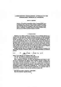
deterministic inputs, often containing a constant or linear function; Φ is the matrix relating the elements of d to x; and ǫk is a 2-dimensional Gaussian random vector with zero mean and variance Ψ that drives the overall process. Note that the states are numbered in decreasing order, so that xk denotes the log-prices of the assets at the k th stage from the end, as depicted in Figure 1 for the two-stage case. Throughout this paper, we restrict attention to the first-order VAR case, but extensions to higher-order VAR systems follow naturally by augmenting the state space. The model given in Eq. 1 is said to exhibit the cointegration property when the matrix defined as Π = Π1 − I is not of full rank. This occurs when the characteristic equation contains a root at unity, possibly endowing each of the underlying time series of xk with a random walk component. The matrix Π1 has one eigenvalue λ1 = 1 and the other with the property that |λ2 | < 1. Since Π is of rank r < 2 and Π 6= 0, it must be true that r = 1, and therefore Π can be expressed as the outer product of two 2 × 1 vectors, as: Π = αβ T .
(2)
The data generated from this random process has finite variance along the direction given by β, and diverging variance in the orthogonal direction, denoted as β ⊥ . The one-dimensional column space of β is commonly referred to as the cointegrating space, while the column space of α is referred to as the space of disequilibrium adjustment forces. It can be shown that for any b in the span of {β}, bT x is a wide-sense stationary random process [6]. We extend the classical Markowitz mean-variance portfolio optimization approach [7] to a two-period setting, in which the objective is to maximize the total expected return of the portfolio summed across both periods, subject to a single constraint on the variance of the total return at the end, rather than a set of constraints on the per-stage returns. Formally, the optimization problem, P0 , is given by: � � ) w1∗ , w2∗ = arg max E w1T r1 + w2T r2 w1 ,w2� P0 � s.t. var w1T r1 + w2T r2 = σ02 , where the per-period vector of individual asset returns, rk , is defined as the change in the log prices, as: rk = ∆xk = xk−1 − xk . The expectation and variance operators are taken with respect to the information available at the starting time, denoted as t2 . The inner product represented by wkT rk denotes the return of the portfolio for stage k. The stages, like the states, are numbered in reverse order, so that wk denotes the relative asset holdings in the k th stage from the end. The portfolio weight vector represents the relative percentage of wealth to allocate to each asset, where a positive weight indicates a long position and negative weight denotes a short position. We allow the portfolio at any stage to be leveraged, i.e. the market value of the
2
x2
1
x1
x0
w2
w1
Stage 2
Stage 1
Initial State
Rebalance Point
Terminal State
t2
t1
t0
Fig. 1. State sequence for two-stage portfolio optimization problem, with rebalancing. The states (log-prices), times, and stages are numbered in decreasing order, so that the subscript indicates the distance from the terminal point.
portfolio may exceed the available wealth, and therefore a budget constraint of the form 1T wk = 1 is not required. The degree of leverage is limited by the allowable risk parameter, σ0 . By introducing a Lagrange multiplier, λ, problem P0 can be rewritten as: � � � � w1∗ , w2∗ , λ∗ = arg max E w1T r1 + E w2T r2 ′ � T � � � w1 ,w�2 ,λT � P0 var w1�r1 + var w�2 r2 . −λ T T 2 +2cov w1 r1 , w2 r2 − σ0 ′
At first glance, it appears that an exact solution to P0 should be easy to compute. However, the portfolio over the last stage, w1 , is itself a random variable, as it depends on the observed value of the state at time t1 , i.e. w1 = f (x1 ). As the nature of this dependence is unknown, it is not possible ′ to immediately compute the terms in P0 that depend on w1 , whether in closed form or by numerical methods. Furthermore, the problem does not map directly into a dynamic programming context [8], as the mean-variance ′ cost function given in P0 is not additive over time due to the non-zero correlation of the per-stage portfolio returns. Additionally, the problem cannot be expressed as the expected utility of the total return due to the presence of the variance operator, which introduces a squared expectation term into the objective function. To address these limitations, ′ we consider a relaxation of problem P0 based on the concept of backwards induction from the DP algorithm. First, the optimal portfolio for the last stage is determined to within a scale factor. Once this direction is established, it is possible to solve for both the direction of the second stage from the end and the optimal variance scheduling scheme, resulting in a suboptimal, but computable solution. III. P ORTFOLIO C ONSTRUCTION Here we solve the two-stage portfolio selection problem by applying the dynamic programming backward recursion. We
4281
47th IEEE CDC, Cancun, Mexico, Dec. 9-11, 2008
ThTA15.3
first consider the tail subproblem consisting of only the last stage, denoted as stage 1 in Figure 1. Looking forward from this time, there is a single decision interval with a holding period of one time step, and therefore we can apply the solution presented in [5] for N = 1, yielding: = a1 Ψ−1 Πx1 = a1 W1 x1 ,
5.6
⊥
x2
5.5
5.4
(3)
Asset 2
w1∗
Simulated VAR(1) Cointegrated System
where a1 is a scale factor or degree of leverage to be determined via enforcement of the total variance constraint. Note that the portfolio direction is a linear function of the state, x1 , and thus by applying the backwards recursion we have determined a particular form for the function w1 = f (x1 ).
x1 5.3
x0 5.2
5.1
3.6
We now seek the optimal portfolio for the second to last stage, given our expression for the portfolio for the last stage. For notational simplicity, let: � � � � w2T (x1 − x2 ) 1 z= , a= . a1 xT1 W1T (x0 − x1 ) The portfolio for the second stage is computed as: � o w2∗ = arg max aT µz − λ aT Σz a − σ02 , P1 w 2
where µz and Σz are the mean vector and covariance matrix of z, respectively, exact expressions for which are derived in Appendix A. The solution to problem P1 is given by: � � � 1 −1 T T ∗ Ψ Π − a1 Π W1 + W1 Π Π1 x2 . (4) w2 = 2λ
This expression for w2 has many interesting properties. First, we observe that Eq. 4 is also a linear function of the current state, and therefore can be rewritten as w2 = W2 x2 . Next, we note that the first term is proportional to Ψ−1 Πx2 , which has identical structure to Eq. 3. This component corresponds to a scaled version of the optimal solution for a single stage problem beginning at time t2 , and thus can be thought of as the “myopic” component. In this light, the second term can be viewed as a correction factor that modifies the myopic solution to account for the uncertainty of the new log-price information, x1 , which becomes available at the rebalance time, t1 . This modification depends both on the direction and scaling of w1 , as is evidenced by the explicit presence of both a1 and W1 factors in Eq. 4. As shown in Appendix A, this correction factor results from the non-zero covariance between the components of the random vector z. In Section IV, we show that this direction modification has the effect of increasing the negative correlation between the returns for stages 1 and 2, enabling an increase in the amount of leverage realized for each period, while maintaining a constant level of total risk. All that remains is to determine the precise variance scheduling scheme, or per-stage leverage amounts that must be exercised in order to meet the total variance constraint. We seek values for the scale factors a1 and λ that maximize
3.7
3.8
3.9
4
4.1
4.2
4.3
4.4
Asset 1 Fig. 2. Geometric view of cointegrated vector autoregressive system in xk space. The three points represent a single path of the random process defined by Eq. 5, beginning from x2 . The data generated according to this model has infinite variance along the β⊥ direction, and finite variance in the β direction. The α vector indicates the direction disequilibrium readjustment forces.
the objective function given in problem P1 . As derived in Appendix A, we find that: � � E[z1 ] − xT2 ΠT Ψ−1 W1,2 x2 1 ∗ a1 = T Ψ−1 W 2λ var [z1 ] − xT2 W1,2 1,2 x2 1 σ0 =q � 2λ T 2 x Ax + A var [z ] − xT WT Ψ−1 W x 2
2
1
1
2
1,2
1,2 2
where A and W1,2 are defined in Equations 6 and 7. While we have chosen to focus here on the two-stage case for simplicity and clarity, extending to the N stage case follows naturally by augmenting the z and a vectors, and continuing to apply the DP backwards recursion. IV. S IMULATION R ESULTS In order to better understand the portfolio directions and variance scheduling scheme derived in Section III, we consider a representative example using data generated from a synthetic model. We compare the portfolios computed using the DP approach to a set of three existing techniques, given by: • The ‘beta’ portfolio: Here the assets are allocated in the direction given by the β vector from the cointegrated VAR model, defined according to Eq. 2, irrespective of the observed state variables. Rebalancing is prohibited, and the portfolio is scaled in order to meet the variance constraint. This scheme is commonly used by practitioners, and is the basis for a wide variety of statistical arbitrage techniques. For additional details, see [2]. • The ‘Markowitz, without rebalancing’ portfolio: The asset allocation rule is formed by considering a single decision interval of length N = 2, and applying the result from [5] for the optimal mean-variance portfolio in a cointegrated VAR system. • A ‘semi-myopic’ portfolio: The result from [5] is independently applied over two consecutive intervals, in
4282
47th IEEE CDC, Cancun, Mexico, Dec. 9-11, 2008
ThTA15.3
order to determine the portfolio directions for each stage. Next, these vectors are appropriately scaled so that the total variance constraint is maintained. The name highlights the fact that the directions are chosen myopically, while the scale factors are not. Additional details are provided in Appendix B. We first contrast the behavior of each trading strategy by examining the second-order statistics of the per-stage and total returns, computed via Monte Carlo simulations. This is followed by a comparison of the four asset allocation schemes using a single, representative sample path.
Beta
Markowitz, without rebalancing
β⊥
5.6
5.5
5.5
5.4
5.4
5.3
5.3
5.2
5.2
5.1
5.1
3.6
3.7
3.8
3.9
4
4.1
4.2
4.3
4.4
3.6
where ǫk ∼ N (0, Ψ) and Ψ = 0.001I. In this system, �T �T α = −0.28 −0.77 and β = −0.66 0.5 , as depicted in Figure 2. The initial log-price pair for �T all of the simulations was chosen to be x2 = 3.9 5.5 , and we are interested in determining the optimal portfolio weights in all four trading scenarios for the case where the total level of the allowed risk is given by σ0 = 0.05, or 5%. The system in Eq. 5 is simulated M =104 times, and the resulting per-stage and total return statistics are given in Table I. The table also displays the correlation coefficient of the inter-stage returns, and it is here that we begin to gain some intuition for the DP solution. As compared to the other approaches, the weights derived via the DP approach achieve a higher negative correlation between the per-period returns, which enables the per-stage variances to be greater in magnitude in contrast to alternative algorithms. In fact, the per-stage variances are each greater than σ02 , while the negative correlation among per-stage returns enables the total variance constraint to still be met, resulting in a higher expected return. Figure 2 illustrates one sample path generated from Eq. 5. The resulting portfolio directions are illustrated in Figure 3, while the exact leverage amounts are presented in Table II. The table also displays the total return achieved by each strategy for this particular sample path. We find that the degree of leverage utilized in the DP approach is greater than all other strategies, which is the main source of the increased realized return. V. E XPERIMENTAL R ESULTS Here we compare the performance of the dynamic programming trading strategy of Section III with the three strategies described in Section IV, using historical price data. The selected dataset from [4] consists of the British Oil (symbol BP.L) stock from the STOXX 50 index, and a replicating portfolio, or tracking index, constructed from the remaining 49 assets, so that the two series exhibit the cointegration property, with no structural breaks or regime
3.7
3.8
3.9
Semi-Myopic
β⊥
5.6
5.5
5.3
4.1
4.2
4.3
4.4
β⊥
5.6
Stage 2 Direction
5.5
Stage 2 Direction
5.4
Stage 1 Direction
5.2
5.1
5.1
3.7
3.8
Stage 1 Direction
5.3
5.2
3.6
4
DP
5.4
Consider the following synthetic VAR(1) model, with no deterministic inputs: � � 1.18 −0.14 xk−1 = xk + ǫk , (5) 0.51 0.62
β⊥
5.6
3.9
4
4.1
4.2
4.3
4.4
3.6
3.7
3.8
3.9
4
4.1
4.2
4.3
4.4
Fig. 3. Comparison of portfolio directions in the xk space for all four trading strategies. Since rebalancing is prohibited in the beta and Markowitz schemes, only a single arrow is shown.
0.05 0.04
1.5σ
0.03 0.02 0.01 0 -0.01 -0.02 -0.03
−1.5σ
-0.04 -0.05
0
10
20
30
40
50
60
70
80
90
100
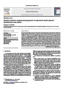
Test Day Fig. 4. Stationary trading indicator signal, z = βT x, used to determine when to enter into test portfolios. Portfolios are bought when |z| > 1.5σz and are sold two periods later.
shifts [3]. Given the BP.L and tracking index datasets, two consecutive 100-day data segments, denoted as xtrain and xtest , were identified in which the parameters of the VAR model remained relatively constant. The closing log prices from November 8, 1999 to March 24, 2000 were used to train the cointegrated VAR model, while the log prices from March 27, 2000 to August 11, 2000 were used to test the trading strategy. A VAR(1) cointegration model with a constant drift term was fit to the training data using the ML estimators described in [6]. A significant decrease in correlation coefficient of the residuals was not achieved by considering higher-order VAR models.
4283
47th IEEE CDC, Cancun, Mexico, Dec. 9-11, 2008 Trading Strategy Beta Markowitz, without rebalancing Semi-Myopic DP
ThTA15.3
Stage 2 Mean Var 0.045 0.0015 0.14 0.0015 0.18 0.002 0.18 0.0045
Stage 1 Mean Var 0.036 0.0016 0.11 0.0021 0.06 0.0009 0.12 0.0039
Correlation -0.19 -0.31 -0.24 -0.70
Total Mean Var 0.081 0.0025 0.25 0.0025 0.24 0.0025 0.30 0.0025
TABLE I S ECOND ORDER STATISTICS OF RETURNS FROM M ONTE C ARLO SIMULATIONS .
Trading Strategy Beta Markowitz, without rebalancing Semi-Myopic DP
Stage 2 Leverage Asset 1 Asset 2 0.99 -0.74 -0.04 -1.22 -0.50 -1.41 0.91 -1.90
Stage 1 Leverage Asset 1 Asset 2 0.99 -0.74 -0.04 -1.22 -0.16 -0.46 -0.33 -0.93
Total Return 0.10 0.29 0.30 0.34
TABLE II ACTUAL P ORTFOLIO L EVERAGE (%
OF INITIAL WEALTH )
Trading Strategy Beta Markowitz, without rebalancing Semi-Myopic DP
VALUES FOR S INGLE S AMPLE PATH ,
Stage 2 Mean Var 0.0207 0.0009 0.0252 0.0014 0.0278 0.0020 0.0275 0.0016
Stage 1 Mean Var 0.0190 0.0006 0.0208 0.0011 0.0346 0.0027 0.0357 0.0028
WITH
σ0 = 0.05.
Total Mean Var 0.0397 0.0018 0.0460 0.0030 0.0624 0.0056 0.0631 0.0054
TABLE III S ECOND ORDER STATISTICS OF RETURNS FROM REAL DATA EXAMPLE .
The trading strategy implemented using this dataset works as follows. For each data point in the test set, we compute a test statistic, z = β T x, as shown in Figure 4. When |z| > 1.5σz , a decision is made to “enter the market”, here resulting in 8 entry points. The portfolio weights for the next two days (stages) are computed according to each strategy using σ0 = 0.05. The per-stage and total return statistics are displayed in Table III. We note that the total variances reported in Table III are not equal to σ02 , which is due not only to the small sample size but also the fact that we are averaging over initial values of x2 . We observe that all of the approaches achieved an average return in the second stage from the end between two and three percent. However, in the last stage from the end, the DP and semimyopic strategies beat the two non-rebalancing strategies by over one percent, due to the fact that they take advantage of the new log-price information that becomes available at the rebalance point. As a result of this truly dynamic trading methodology, these strategies achieve a higher total return for each initial condition, while maintaining a constant level of total risk. As we saw in the Monte Carlo simulations of Section IV, it is the DP strategy that is able to achieve the highest expected return, due to the increase in the negative correlation of the inter-stage returns.
beginning of the second to last stage, time t2 . Let � � � � z2 w2T (x1 − x2 ) z= = , z1 xT1 W1T (x0 − x1 ) and we have: E[z2 ]
= w2T E [Πx2 + ǫ2 ] = w2T Πx2 , � � E[z1 ] = E xT1 W1T (x0 − x1 ) � � = E xT1 W1T Πx1 + xT1 W1T ǫ1 � � = E xT1 W1T Πx1 � � = xT2 ΠT1 W1T ΠΠ1 x2 + trace W1T ΠΨ ,
where W1 = Ψ−1 Π. We now compute each of the terms in Σz . The variance of z2 is easily computed as: � � var [z2 ] = var w2T (x1 − x2 ) = w2T Ψw2 .
In order to compute the variance of z1 , we invoke the law of total variance, as: var [z1 ]
A PPENDIX A In this Appendix we derive expressions for µz , Σz , w2 , a1 , and λ. We begin with µz , and recall that all expectations are computed with respect to the information available at the
� � = E w2T (x1 − x2 )
= var [ E [z1 | x1 ]] + E [ var [z1 | x1 ]] � � � � = var xT1 W1T Πx1 + E xT1 W1T ΨW1 x1 .
We now define the symmetric matrix A as:
4284
A , W1T Π = ΠT Ψ−1 Π = W1T ΨW1 ,
(6)
47th IEEE CDC, Cancun, Mexico, Dec. 9-11, 2008
ThTA15.3
Accordingly, we can express the variance of z1 as: var [z1 ]
A PPENDIX B
� � � � = var xT1 Ax1 + E xT1 Ax1
= 4xT2 ΠT1 AΨAΠ1 x2 + 2trace [AΨAΨ] +xT2 ΠT1 AΠ1 x2 + 2trace [AΨ] Lastly, the covariance is computed as: cov [z1 , z2 ] = E [z2 z1 ] − E [z2 ] E [z1 ] � � = E w2T (Πx2 + ǫ2 ) z1 − E [z2 ] E [z1 ]
= w2T E [ǫ2 z1 ] � � = w2T E ǫ2 xT1 W1T (Πx1 + ǫ1 ) � � = w2T E ǫ2 xT1 W1T Πx1 h i T = w2T E ǫ2 (Π1 x2 + ǫ2 ) W1T Π (Π1 x2 + ǫ2 ) � = w2T Ψ ΠT W1 + W1T Π Π1 x2
= w2T W1,2 x2 .
(7)
Here we present the problem formulation and solution for the semi-myopic approach. The two stage problem is solved as two consecutive one stage problems, in which the direction of the portfolio for each stage is selected to be equal to the optimal action for a single stage problem, with no consideration given to past or future stages. Once these directions are computed, the degree of leverage is determined so that the total expected return is maximized while ensuring that the variance constraint is met. Applying the approach in [5] independently for each period, we have: w2∗ w1∗
= a2 Ψ−1 Πx2 , = a1 Ψ−1 Πx1 ,
where the ak ’s are scale factors that determine the degree of leverage of the portfolio at stage k. These factors are determined by solving problem P2 , as: � o a∗1 , a∗2 = arg max a′T µz′ − λ a′T Σz′ a′ = σ02 , P2 a1 ,a2
Now that we have all of the terms in µz and Σz , we can compute w2∗ by differentiating the objective function in Problem P1 with respect to w2 , as: 0 w2∗
= Πx2 − λ2Ψw2 − 2λa1 W1,2 x2 1 −1 = Ψ (Πx2 − 2λa1 W1,2 x2 ) 2λ � � � 1 −1 T T Ψ Π − a1 Π W1 + W1 Π Π1 x2 . = 2λ
where:
z′ a′
The scale factor applied to the last stage can be found by differentiating the objective function in Problem P1 with respect to a1 , as:
� xT2 ΠT Ψ−1 (x1 − x2 ) , xT1 ΠT Ψ−1 (x0 − x1 ) � � a2 , = a1 =
�
and µz′ and Σz′ refer to the mean vector and covariance matrix of z′ , respectively. The optimal scale factors are: � ∗� 1 −1 a2 Σ ′ µ ′ = a∗1 2λ z z σ0 1 = q . 2λ µT Σ−1 µ z′
0 = E[z1 ] − 2λa1 var [z1 ] − 2λcov [z1 , z2 ] = E[z1 ] − 2λa1 var [z1 ] − 2λw2T W1,2 x2 = E[z1 ] − 2λa1 var [z1 ] − xT2 ΠT Ψ−1 W1,2 x2 � +2λa1 xT2 ΠT1 ΠT W1 + W1T Π W1,2 x2 � � E[z1 ] − xT2 ΠT Ψ−1 W1,2 x2 1 a∗1 = T Ψ−1 W 2λ var [z1 ] − xT2 W1,2 1,2 x2 1 A1 = 2λ
z′
z′
R EFERENCES
[1] J. Stock and M. Watson, “Testing for common trends,” Journal of the American Statistical Association, vol. 83, no. 404, pp. 1097–1107, 1988. [2] Y. Kawasaki, S. Tachiki, H. Udaka, and T. Hirano, “A characterization of long-short trading strategies based on cointegration,” Proceedings of the 2003 International Conference on Computational Intelligence for Financial Engineering (CIFEr2003), pp. 411–416, 2003. 1 Finally, the value of the quantity 2λ is found to be: [3] C. Alexander and A. Dimitriu, “Index and statistical arbitrage,” Journal of Portfolio Management, vol. 31, no. 2, pp. 50–63, 2005. [4] A. N. Burgess, Applied Quantitative Methods for Trading and Investσ02 = w2T Ψw2 + a21 var [z1 ] + 2a1 w2T W1,2 x2 ment, chapter Using Cointegration to Hedge and Trade International � �2 h Equities, Wiley, 2003. 1 T xT2 (Π − A1 W1,2 ) Ψ−1 (Π − A1 W1,2 ) x2 [5] M. Rudoy and C. Rohrs, “Optimal portfolio construction in cointegrated = 2λ vector autoregressive systems,” Proceedings of the 2008 American i Control Conference (ACC), 2008. T 2 T −1 +A1 var [z1 ] + 2A1 x2 (Π − A1 W1,2 ) Ψ W1,2 x2 [6] S. Johansen, Likelihood-Based Inference in Cointegrated Vector Autoregressive Models, Oxford University Press, New York, 1995. [7] H. Markowitz, “Portfolio selection,” Journal of Finance, vol. 7, no. 1, pp. 77–91, 1952. 1 σ0 [8] D. Bertsekas, Dynamic Programming and Optimal Control, Athena , =q � Scientific, Belmont, MA, 2000. 2λ T T T 2 −1
x2 Ax2 + A1 var [z1 ] − x2 W1,2 Ψ
W1,2 x2
where A is defined according to Eq. 6.
4285