A Dynamic Programming Approach to. Reconstructing Building Interiors. Alex Flint, Christopher Mei, David Murray, and Ian Reid. Dept. Engineering Science.
A Dynamic Programming Approach to Reconstructing Building Interiors Alex Flint, Christopher Mei, David Murray, and Ian Reid Dept. Engineering Science University of Oxford Parks Road, Oxford, UK {alexf,cmei,dwm,ian}@robots.ox.ac.uk
Abstract. A number of recent papers have investigated reconstruction under Manhattan world assumption, in which surfaces in the world are assumed to be aligned with one of three dominant directions [1–4]. In this paper we present a dynamic programming solution to the reconstruction problem for “indoor” Manhattan worlds (a sub–class of Manhattan worlds). Our algorithm deterministically finds the global optimum and exhibits computational complexity linear in both model complexity and image size. This is an important improvement over previous methods that were either approximate [3] or exponential in model complexity [4]. We present results for a new dataset containing several hundred manually annotated images, which are released in conjunction with this paper.
1
Introduction
In this paper we investigate the problem of reconstructing simple geometric models from single images of indoor scenes. These scene models can be used to distinguish objects from background in recognition tasks, or provide strong global contextual cues about the observed scene (e.g. office spaces, bedrooms, corridors, etc.). Point clouds provided by structure–from–motion algorithms are often sparse and do not provide such strong indicators. Compared to a full dense reconstruction, the approach is computationally more efficient and is less sensitive to large texture–less regions typically encountered in indoor environments. The past few years have seen considerable interest in the Manhattan world assumption [1, 2, 4, 3, 5], in which each surface is assumed to have one of three possible orientations. Making this assumption introduces regularities that can improve the quality of the final reconstruction [3]. Several papers have also investigated indoor Manhattan models [4–6] (a sub–class of Manhattan models), which consist of vertical walls extending between the floor and ceiling planes. A surprisingly broad set of interesting environments can be modelled exactly or approximately as indoor Manhattan scenes [5]. It is with this class of scenes that this paper is concerned. The present work describes a novel and highly efficient algorithm to obtain models of indoor Manhattan scenes from single images using dynamic programming. In contrast to point cloud reconstructions, our algorithm assigns semantic
2
Alex Flint, Christopher Mei, David Murray, and Ian Reid
labels such as “floor”, “wall”, or “ceiling”. We show that our method produces superior results when compared to previous approaches. Furthermore, our algorithm exhibits running time linear in both image size and model complexity (number of corners), whereas all previous methods that we are aware of [4, 5] are exponential in model complexity. The remainder of the paper is organised as follows. Section 2 describes previous work in this area and section 3 outlines our approach. In section 4 we pose the indoor Manhattan problem formally, then in section 5 we develop the dynamic programming solution. We present experimental results in section 6, including a comparison with previous methods. Concluding remarks are given in the final section.
2
Background
Many researchers have investigated the problem of recovering polyhedral models from line drawings. Huffman [7] detected impossible objects by discriminating concave, convex, and occluding lines. Waltz [8] investigated a more general problem involving incomplete line drawings and spurious measurements. Sugihara [9] proposed an algebraic approach to interpreting line drawings, while the “origami world” of Kanade [10] utilised heuristics to reconstruct composites of shells and sheets. Hoiem et al. [11] and Saxena et al. [12] have investigated the single image reconstruction problem from a machine learning perspective. Their approaches assign pixel–wise orientation labels using appearance characteristics of outdoor scenes. Hedau et al. [6] extend this to indoor scenes, though their work is limited to rectangular box environments. The work most closely related to our own is that of Lee et al. [4], which showed that line segments can be combined to generate indoor Manhattan models. In place of their branch–and–bound algorithm, our system uses dynamic programming to efficiently search all feasible indoor Manhattan models (rather than just those generated by line segments). As a result we obtain more accurate models, can reconstruct more complex environments, and obtain computation times several orders of magnitude faster than their approach, as will be detailed in Section 6. Furukawa et al. [3] used the Manhattan world assumption for stereo reconstruction. They make use of multiple calibrated views, and they search a different class of models, so their approach is not comparable to ours. Barinova et al. [13] suggested modelling outdoor scenes as a series of vertical planes. Their models bear some similarity to ours but they cannot handle occluding boundaries, and their EM inference algorithm is less efficient that our dynamic programming approach. Felzenszwalb and Veksler [14] applied dynamic programming to a class of pixel labelling problems. Because they optimise directly in terms of pixel labels their approach is unable to capture the geometric feasibility constraints that our system utilises.
A Dynamic Programming Approach to Reconstructing Building Interiors
3
(b)
(a)
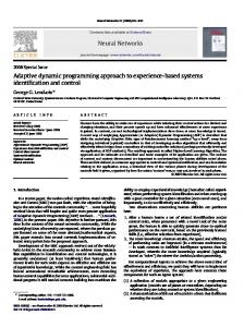
Fig. 1: (a) Three input images and the indoor Manhattan models we seek. Notice how each image column intersects exactly one wall. (b) The mapping Hc→f transfers points between the ceiling and floor.
3
Outline of Proposed Approach
Our goal is to reconstruct an indoor Manhattan model from a single image. Three example images and the models we seek for them are shown in Figure 1a. A perfectly uncluttered environment such as that shown in the third column of Figure 1a could be represented exactly by an indoor Manhattan model, though in general we expect to encounter clutter and our goal in such cases is to recover the boundaries of the environment in spite of this distraction. That is, we aim to completely ignore all objects within the room and reconstruct the bare room boundaries, in contrast to most previous approaches that aim to reconstruct the entire scene. This choice is due to our intention of using the models as input for further reasoning. The Manhattan world assumption states that world surfaces are oriented in one of three mutually orthogonal directions [1]. The indoor Manhattan assumption further states that the environment consists of a floor plane, a ceiling plane, and a set of walls extending vertically between them [4]. Each wall therefore has one of two possible orientations (ignoring sign), and each corner1 is either concave, convex, or occluding, as depicted in Figure 3. Indoor Manhattan models are interesting because they can represent many indoor environments approximately or exactly, yet they introduce regularities to the reconstruction problem that makes possible a left–to–right decomposition of the scene, on which the dynamic programming algorithm developed in this paper rests. Our approach to reconstructing indoor Manhattan environments consists of the following five steps: 1. Identify three dominant surface orientations. (Section 3.1) 2. Identify the floor and ceiling planes. (Section 3.2) 1
we use “corner” throughout this paper to refer to the intersection of two walls, which appears as a line segment in the image
4
Alex Flint, Christopher Mei, David Murray, and Ian Reid
3. Rectify vertical lines. (Section 3.3) 4. Obtain weak orientation estimates. (Section 3.4) 5. Estimate the final model. (Sections 4 and 5)
3.1
Identifying dominant directions
We identify three dominant directions by estimating mutually orthogonal vanishing points in the image. Our approach is similar to Koseck`a and Zhang [2], in which k–means clustering provides an initial estimate that is refined using EM. We assume that the vertical direction in the world corresponds to the vanishing point with largest absolute y–coordinate, which we label vv . The other two vanishing points are denoted vl and vr . If the camera intrinsics are unknown then we construct the camera matrix K from the detected vanishing points by assuming that the camera centre is at the image centre and choosing a focal length and aspect ratio such that the calibrated vanishing points are mutually orthogonal.
3.2
Identifying the floor and ceiling planes.
An indoor Manhattan scene has exactly one floor and one ceiling plane, both with normal direction vv . It will be useful in the following sections to have available the mapping Hc→f between the image locations of ceiling points and the image locations of the floor points that are vertically below them (see Figure 1b). Hc→f is a planar homology with axis h = vl ×vr and vertex vv [15] and can be recovered given the image location of any pair of corresponding floor/ceiling points (xf , xc ) as Hc→f = I + µ
vv hT , vv · h
(1)
where µ =< vv , xc , xf , xc × xf × h > is the characteristic cross ratio of Hc→f . Although we do not have a priori any such pair (xf , xc ), we can recover Hc→f using the following RANSAC algorithm. First, we sample one point x ˆc from the region above the horizon in the Canny edge map, then we sample a second point x ˆf collinear with the first and vv from the region below the horizon. ˆ c→f as described above, which we then score We compute the hypothesis map H ˆ c→f maps onto other edge pixels (according by the number of edge pixels that H to the Canny edge map). After repeating this for a fixed number of iterations we return the hypothesis with greatest score. Many images contain either no view of the floor or no view of the ceiling. In such cases Hc→f is unimportant since there are no corresponding points in the image. If the best Hc→f output from the RANSAC process has a score below a threshold kt then we set µ to a large value that will transfer all pixels outside the image bounds. Hc→f will then have no impact on the estimated model.
A Dynamic Programming Approach to Reconstructing Building Interiors
3.3
5
Rectifying vertical lines
The algorithms presented in the remainder of this paper will be simplified if vertical lines in the world appear vertical in the image. We therefore warp images according to the homography vv × e3 , vv H= e3 = [0, 0, 1]T . (2) vv × e3 × vv 3.4
Obtaining weak orientation estimates
Our algorithm requires a pixel–wise surface orientation estimate to bootstrap the search. Obtaining such estimates has been explored by several authors [4, 11, 12]. We adopt the simple and efficient line–sweep approach of Lee et al. [4], which produces a partial labelling of the image in terms of the three Manhattan surface orientation labels (corresponding to the three Manhattan orientations in the image). We denote this orientation map o : Z2 → {l, r, v, ∅} where ∅ represents the case in which no label is assigned and l, r, and v correspond to the three vanishing points {vl , vr , vv }. Note that our algorithm is is not dependent on the manner in which o is obtained; any method capable of estimating surface orientations from a single image, including the work of Hoiem [11] or Saxena [12], could be used instead. We generate three binary images Ba , a ∈ {l, r, v} such that Ba (x) = 1 if and only if o(x) = a. We then compute the integral image for each Ba , which allows us to count the number of pixels of a given orientation within any rectangular sub–image in O(1) time. This representation expedites evaluation of the cost function described later.
4
Formulation of reconstruction problem
Consider the indoor Manhattan scenes shown in Figure 1a. Despite the complexity of the original images, the basic structure of the scene as depicted in the bottom row is simple. In each case there is exactly one wall between any two adjacent corners1 , so any vertical line intersects at most one wall. This turns out to be a general property of indoor Manhattan environments that arises because the camera must be between the floor and ceiling planes. Any indoor Manhattan scene can therefore be represented as a series of one or more wall segments in order from left to right. Given the warp performed in the Section 3.3, corners are guaranteed to appear vertical in the image, so can be specified simply by an image column. Furthermore, given the mapping Hc→f from Section 3.2 the image location of either the top or bottom end–point of a corner (i.e. the intersection of the wall with the ceiling or floor respectively) is sufficient to specify both and thereby the line segment representing that corner. Without loss of generality we choose to represent corners by their upper end–point. A wall segment can then be specified
6
Alex Flint, Christopher Mei, David Murray, and Ian Reid
? l
(a)
r
(b)
r
l
(c)
Fig. 2: (a) The row/column indices ci , ci+1 , ri , together with the vanishing point index ai ∈ {l, r} are sufficient via the homology Hc→f to determine the four vertices defining a wall. (b) An illustration of the model M = {c1 , (r1 , a1 ), ..., c4 , (r4 , a4 ), c5 }. (c) A partial model covering columns to c1 to c4 with several feasible (green dashed) and infeasible (red dashed) wall segments.
by its left and right corners, together with its associated vanishing point (which must be either vl or vr ), as illustrated in Figure 2a. This leads to a simple and general parametrisation under which we represent an indoor Manhattan model M as an alternating sequence of corners and walls (c1 , W1 , c2 , W2 , ..., Wn−1 , cn ), ci < ci+1 . Each corner ci is the column index at which two walls meet, and each wall Wi = (ri , ai ) comprises an orientation ai ∈ {l, r}, which determines whether its vanishing point is vl or vr , and a row index ri , at which its upper edge meets the corner to its left (see Figure 2b). Hence the upper–left corner of the ith wall is (ci , ri ), which, together with its vanishing point vai , fully specifies its location in the image. Clockwise from top–left the vertices of the ith wall are pi = [ci , ri , 1]T , qi = pi×vai×[1, 0, −ci+1 ]T , ri = Hc→f qi , si = Hc→f pi . (3) A model M generates for each pixel x a predicted surface orientation gM (x) ∈ {l, r, v} corresponding to one of the three vanishing points {vl , vr , vv }. We compute gM by filling quads corresponding to each wall segment, then filling the remaining area with the floor/ceiling label v. Not all models M are physically realisable, but those that are not can be discarded using simple tests on the locations of walls and vanishing points as enumerated by Lee et al. [4]. The reader is referred to their paper for details; the key result for our purposes is that a model is feasible if all of its corners are feasible, and the feasibility of a corner is dependent only on the immediately adjoining walls. 4.1
Formalisation
We are now ready to formalise the minimisation problem. Given an input image of size W × H and an initial orientation estimate o, the pixel–wise cost Cd (x, a)
A Dynamic Programming Approach to Reconstructing Building Interiors
7
measures the cost of assigning the label a ∈ {l, r, v} to pixel x. We adopt the simple model, ( 0, if o(x) = a or o(x) = ∅ . (4) Cd (x, a) = 1, otherwise The cost for a model M consisting of n corners is then the sum over pixel– wise costs, X C(M) = nλ + Cd (x, M(x)) (5) x∈I
where λ is a constant and nλ is a regularisation term penalising over–complex models. We seek the model with least–cost M∗ = argmin C(M) .
(6)
M
where implicit in (5) is the restriction to labellings representing indoor Manhattan models, since only such labellings can be represented as models M. Figure 1a shows optimal models M∗ for three input images.
5
Proposed algorithm
In this section we present a dynamic programming solution to the minimisation problem posed in the previous section. We develop the algorithm conceptually first, then formalise it later. We have already seen that every indoor Manhattan scene can be represented as a left–to–right sequence of wall segments, and every image column intersects exactly one wall segment. As a result, the placement of each wall is “conditionally independent” of the other walls given its left and right neighbours. For example, Figure 2c shows a partial model as well as several wall segments that could be appended to it. Some of the candidates are feasible (green dashes) and some are not (red dashes); however, note that once the wall segment from c3 to c4 is fixed, the feasibility of wall segments following c4 is independent of choices made for wall segments prior to c3 . This leads to a decomposition of the problem into a series of sub–problems of the form “find the minimum–cost partial model that terminates2 at x = (c, r)”. To solve this we enumerate over all possible walls W that have top–right corner at x, then for each we recursively solve the sub–problems for the partial model terminating at each x0 , where x0 ranges along the left edge of W . This recursive process eventually reaches the left boundary of the image since x0 is always strictly to the left of x, at which point the recursion terminates. As is standard in dynamic programming approaches, the solution to each sub–problem is cached to avoid redundant computation. To solve the complete minimisation (6) we simply solve the sub–problems corresponding to each point on the right boundary of the image. 2
A model “terminates” at the top–right corner of its right–most wall.
8
Alex Flint, Christopher Mei, David Murray, and Ian Reid
Fig. 3: Three models satisfying constraints 1–3 for the sub–problem fin (x, y, a, k). Only one will satisfy the least–cost constraint.
We now formalise the dynamic programming algorithm. Let fin (x, y, a, k) be the cost of a model M+ = {c1 , W1 , ..., Wk−1 , ck } such that 1. 2. 3. 4.
ck = x (i.e. the model terminates at column x), Wk−1 = (y, a) (i.e. the model terminates at row y with orientation a), M+ is feasible, and M+ has minimal cost among all such models. We show in the additional material that if a model M = {c1 , W1 , ..., Wk−1 , ck }
(7)
is a solution to the sub–problem fin (ck , rk , ak , k), then the the truncated model M0 = {c1 , W1 , ..., Wk−2 , ck−1 }
(8)
is a solution to the sub–problem fin (ck−1 , rk−1 , ak−1 , k − 1). In light of this we introduce the following recurrence relation: � � fin (x, y, a, k) = 0 min0 0 fin (x0 , y 0 , a0 , k − 1) + Cw , (9) x