1
ACCV2002: The 5th Asian Conference on Computer Vision, 23--25 January 2002, Melbourne, Australia. (oral)
A Face Recognition Method Based on Local Feature Analysis Feng Jiao 1, Wen Gao1 ,2, Xilin Chen2, Guoqin Cui1, Shiguang Shan1 1 ICT-YCNC FRTJDL, Institute of Computing Technology, CAS, Beijing 100080,China 2 Department of Computer Science, Harbin Institute of Technology, Harbin, 150001, China E-Mail:{fjiao, wgao}@ict.ac.cn;
[email protected];{ cgq, sgshan}@ict.ac.cn
Abstract Elastic Bunch Graph Matching has been proved effective for face recognition. But the recognition procedure needs large computation. Here we present an automatic face recognition method based on local feature analysis. The local features are firstly located by the face structure knowledge and gray level distribution information, rather than searching on the whole image as it does in Elastic Bunch Graph Matching. Thus the whole computation is greatly decreased. Then the features are adjusted using a data structure named Face Bunch Gra ph. The face is represented by Gabor jets of the features and their spatial distances. Several distance metrics are tested and the results are given.
1. Introduction Face recognition technology can be used in wide range of applications such as identity authentication, access control, and surveillance. Interests and research activities in face recognition have increased significantly over the past twenty years [1][2]. It has been widely recognized that human being recognize people mainly based on local features such as eyes, nose, and mouth, and their spatial arrangement. In this paper, an automatic face recognition system based on local features analysis is presented. In Geometric Feature-based methods [1][3], facial features such as eyes, nose, month, and chin are detected. Properties and relations such as areas, distances, and angles, between the features are used as the descriptors of faces. Although being economical and efficient in achieving data reduction and
insensitive to variation in illumination and viewpoint, this class of methods relies heavily on the extraction and measurement of facial features. Unfortunately, feature extraction and measurement techniques and algorithms developed to date have not been reliable enough to cater to this need [4]. In our system, features are firstly detected using some geometric and gray level distribution information. But it is not accurate enough for face recognition. So we use a data structure named Face Bunch Graph to calibrate it. These features are mainly focused on the internal area, for the internal features are more important for recognition than external features. And we ignore the hairstyle and the background of an image, although sometimes it is used for recognition. After the feature is accurately calibrated, a set of complex vectors is obtained by calculating the complex coefficients in the feature points. The face is represented by these vectors. The similarity expression is given and the result is calculated.
2. Facial features detection and extraction 2.1 Location of the irises In our system, the detecting of the features is based on the location of the two irises. That is mainly because the irises are most obvious in the face image and their accuracy can be guaranteed. In a given face area, the image is two-binary, and some pair of connected areas are founded. By using the face structural knowledge, we can find a particular pair of connected area L and R where the two eyes locate. In the binary image B and binary edge image E of the area L and R, we can get the description of two eyes area
2
Rng = ( x, y ) | B( x, y ) = 0, ∑ E (i , j ) > θ ( i , j )∈Ω Ω is the eight pixels set around the point (x,y).
(1)
Then we get the cursory sets of the two eyes. The center of the points set is calculated and we get some candidates of the irises. For each candidate, we calculate the following support function in the edge image E
Sp =
1 N
A is the annulus area with
∑E
( x, y )∈ A
(2)
( x ,y )
R1 ≤ r ≤ R2
And the one, which has maximum support function, is chosen as the iris.
PLeftIris = arg( Max S p ) p∈ Rngleft
(3)
According to the experiments results, we will get a similar curve unless there is much noise or very heave bear. Gauss smoothing is used and the minimum point of the curve is calculated. Gauss smoothing is done as follow: h (i ) = f ( i ) * g ( i ) = ∑ f (i ) g ( i − j ) (5) j : g ( x ) = exp( − x 2 /( 2 s 2 )) and the minimum point of the curve is got by calculating the first derive and the second derive. h ′ ( i ) = ( h ( i + 1 ) − h ( i − 1)) / 2 (6) h ′′ ( i ) = h ( i + 1 ) + h ( i − 1) − 2 h ( i) then we get the minimum point set (7) S = {i | h ′(i + 1) h ′ (i + 1) = 0} and we can get the mouth center point
m = arg min { f ( i ), ∀ i ∈ S } i
PLeftIris = arg( Max S p ) p∈Rngright
(4)
(8)
Other feature points are located as the process above. The detailed method can be found in [5].
After the two irises are located, we need to rotate the image in order to make it easier to locate the others features. We rotate the image based on the center of the face rather than the image. The center of the face is calculated by using the position of the two irises center position and the face structural knowledge.
2.2 Location of the other Features
Figure 2. samples of results of feature location
After the location of the irises, we can get the rough location area of the other features based on the statistic knowledge of the face. After the integral projection of the face, there is some particular characteristic in the feature point. We can use this to search in the area and find the position. As to the location of the mouth center, first we get the area
Here we totally use 26 points, these points are mainly focus on the internal face area, for the internal features are more important for recognition than external features. And more features are focused on the upper part of the face, for it has been founded that the upper part of the face is more useful for face recognition than the lower part of the face [2].
3. Facial feature adjusting average gray value
The features got from the above algorithm are not accurate enough for recognition. So we use a data structure named Face bunch graph to adjust it. coordinate
a)
3.1 Gabor convolution and Gabor jets
b)
Figure 1. Integral Project Curve and Result of Mouth Locating (a) Region for Integral and Corresponding Result (b) Integral Project Curve of the mouth, then we do integral projection to this area and get an integral project curve as showed in the Figure 1.
The using of the 2D Gabor wavelet representation in computer vision was pioneered by Daugman in 1980’s [8]. The Gabor wavelet representation allows description of spatial frequency structure in the image while preserving information about spatial relations. A complex-valued 2D Gabor function is a plane wave restricted by a Gaussian envelope:
3
k 2j x 2 r ϕ j (x ) = k 2j exp − 2σ 2
r kj =
( )=( k jx k jy
r r σ2 exp i k x − exp − j 2
)
kv cosφu kv sinφu
kv = 2
−
v+2 π 2
(9)
here 5 frequencies and 8 orientations are used
φu = u
π , j = u + 8v , v = 0,...,4 , u = 0 ,..., 7 8
can estimate the displacement between two jets up to 8 pixels [6]. By comparing the jet bunch of each feature, we can get the best fitting jet at a new position. These new positions are used for recognition. This representation is chosen for its biological relevance and technical properties. The Gabor kernels resemble the receptive field profiles of simple cells in the visual pathway. They are localized in both space and frequency domains and achieve the lower bound of the space-bandwidth product as specified by the uncertainty principle [7].
3.2 Elastic bunch graph
r
r
By maximizing the similarity S φ in its Taylor expansion, we
In an image a given pixel x with gray level L x , the convolution can be defined as
r r r r r J j (x ) = ∫ L(x ' )ϕj (x − x ' )d 2 x '
(10)
When all 40 kernels are used, 40 complex coefficients are provided. We called it as a jet, which is used to represent the local features.
( )
In order to make the facial feature accurately located, a data structure face bunch graph is used. To represent all wide ranges of local features, we store different jets of the local features. Such as for left eye center jets, we collect many left eyes center jets from different people, and different shaped with widely opened or closed, and also with different illumination. The graph nodes are these jets, and the edges are labeled with the averages of distance vectors.
3.3 Features adjusting
magnitudes a j ( x ) vary slowly with position, and phases
r φ j ( x ) rotate at a rate approximately determined by the
The features we get in the section 2 are not accurate enough for recognition and need to be adjusted. First we adjust the local features individually. In the each point of the feature, the Gabor complex i coefficients J k are calculated and its displacement is also
frequency of the kernel.
estimated by using the similarity function
J j = a j exp iφ j , where
A jet can be expressed as
r
Two Similarity functions are phase-insensitive similarity function:
∑a a
S a (J , J ) =
j
applied.
2 j
Sφ (J , J ' ) =
j
j
' j
'2 j
j
j
is the Gabor jet of the i image in the FBG. In i'
(11)
rr cosφ j − φ 'j − d k j 2 '2 ∑ aj ∑ aj
)
the new position we get above, the Gabor jet J k and it
It varies smoothly with the change of the position and we use it for recognition. Another is phase-sensitive similarity function:
∑a a
where J
(
th
FBGi
∑ a ∑a j
is
' j
j
'
One
FBGi K
Sφ J ki , J KFBGi ,
(12)
j
It changed quickly with location and it is used for feature adjusting.
similarity with J K
(
i'
FBGi
of S a J k , J K
) is also calculated.
The best fitting point is chosen as the feature point.
3.4 Addition adjusting Here we assume that most of the points located above are near the 8 pixels to the accurate position. And in our experiment it is true that most often it do so. But it happens that some of them will be out of the 8 pixels and this feature is sure to located wrong. Then we need additional adjusting. Normally it happens in the mouth and chin. Here we use the knowledge of the facial structure as described in the above to tell whether a facial feature is localized correctly or not. If the feature is not correctly lo calized, we
4
search the area where the feature may locate and use the follow similarity function:
S φ (I , FBG −
λ E
E
∑ e =1
)=
(∆ X
I e
L
1 L
Max ∑ k =1
− ∆X
(∆ X
FBG e 2 FBG e
)
S m ( J kI , J
FBG K
i
)
i
)2
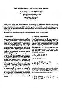
Figure 3. samples of our face database.
(13) where L is the number of the nodes of FBG and E is the number of edges of FBG. λ is an experimental value that determines the relative importance of facial feature similarities and the topography term. In [6][9], a coarse to fine approach method is applied to find the fiducial points. It searches the whole image and adjusting for several times. One of its drawbacks is the large computation. In our system, the fiducial points are first estimated, and normally their distance to the accurate position is not more than 8 pixels , and thus the adjusting procedure is quick.
Another experiment is tested on the Olivetti Research Ltd. Database (400 images of 40 individuals, 10 Images per individual). When one image is tested, the other 9 images are chosen as the train images. Each of the images is tested once in our experiments.
Table 1 result of the experiment 1(De is the result using Euclidian metric, Dabc is the method using angle between vectors, Dcbd is the method using city block distance metric, Eigen+ NN is the method using EigenFace and NN)
4. Recognition and experimental results Local feature method After the features are accurately located, the face is represented by the Gabor jets on these feature points and their spatial distances. For the measure of distance in feature space, we use some metrics. A natural choice is the geometric metric.
r r de ( x, y) =
∑ (x − y )
De 92.3%
Dabc 92.7%
Dcbd 93.3%
EigenFace+NN
86.7%
2
i
(14)
i
i
Another metric is angle between vectors.
r r d abc ( x, y) = cos−1
r r x⋅y r r x y
(15)
And the city block distance metric (CBD)
r r dcbd (x , y ) = ∑ xi − yi
(16)
The first experiment was tested for recognizing people from single frontal view picture. For in most cases, we normally have only one picture for training. The database we use has 300 people, each person have 2 pictures, one for training and the other for test. The two pictures differ slightly in face expression and light. For comparison, we also use EigenFace+NN method.
Figure 4. samples of ORL face database.
Table 2 result of the experiment 2 Local feature method EigenFace+KNN
De
Dabc
Dcbd
93.75%
93.5%
94.5%
91.5%
5
We can see that this method is better than the Eigenface method in our experiments.
5. Conclusion and discussion In the traditional EGM method, the large computation is mainly focus on the extraction of the model graphs from the probe images. In order to search the feature points, it uses a coarse to fine method. It needs translation, scale, aspect ratio, and local distortions [6]. In our method, the features are located using the face structure knowledge and gray level distribution information. And then in the adjusting procedure, the computation is very small. And most feature points are well located and only a few need further adjusting. In our system, about average 2.8 points out of 26 points need further adjusting. (mainly locate in the lower part of the face). So the third procedure also requires little time. In this paper, an automatic face recognition me thod based on local feature analysis is presented. The face in an image is detected first and the local features are located using the face structure knowledge and gray level distribution information. Then the features are further adjusted using a data structure Face Bunch Graph. The face is represented by the Gabor jets of the features and their spatial distances. Several distance metrics are tested and the results are given. This system relies on the accurate detection of the face and location of the features, although we can adjust it later. But if the quality of the image is too bad and the face can’t be found, the system will fail. And we solve this problem by manual locating these features.
6. Acknowledgments This research is sponsored partly by Natural Science Foundation of China (No.69789301), National Hi-Tech Program of China (No.863-306-ZD03-01-2), 100 Talents Foundation of Chinese Academy of Sciences, and SiChuan Chengdu Yinchen Net. Co.
References [1] R.Chellappa, C.L. Wilson, and S. Sirohey. Hunam and machine recogniton of faces: A servey. Proc. IEEE, 83:705-741, May 1995 [2] W. Zhao, R. Chellappa, A. Rosenfeld, P.J. Phillips Face Recognition: A Literature Survey. url="citeseer.nj.nec.com/374297.html"
[3] R. Brunelli and T. Poggio. Face recogniton: Features versus templates. IEEE Transactions on Pattern Analysis and Machine Intelligence, 15:1042-1052,1993. [4] I.J.Cox, J.Ghosn, and P.Yianilos. Feature-based face recognition using mixture-distance. CVPR, pages 209-216,1996. [5] Shan Shiguang, Gao wen, Chen Xilin. Facial Feature Extraction Based on Facial Texture Distribution and Deformable Template. Journal of Software, Vol. 12 No.4 April 2001, 571-577. [6] Laurenz Wiskott, jean-Marc Fellous, Norbert Kruger, and Christoph von der Malsburg, Face Recognition by Elastic Graph Matching, IEEE Transations on Pattern Analysis and Machine Intelligence, Vol. 19, no, 7,July 1997. [7] R.N.Bracewell, The Fourier Transform and Its Application, New York, McGraw-Hill, 1978 [8] Daugman, J. G. (1998). Complete discrete 2-D Gabor transform by neural network for image analysis and compression. IEEE Trans. On Acoustics, Speech and Signal Processing, 36(7):1169-1179 [9] R.Liao and S.Li Face. Recgnition Based on Multiple Facial Features. Proceedings of the Fou rth International conference on Automatic Face and Gesture Recognition:239-244