Face Recognition with Decision Tree-based Local ... - Semantic Scholar

Face Recognition with Decision Tree-based Local Binary Patterns ´ Daniel Maturana, Domingo Mery and Alvaro Soto Department of Computer Science, Pontificia Universidad Cat´ olica de Chile

Abstract. Many state-of-the-art face recognition algorithms use image descriptors based on features known as Local Binary Patterns (LBPs). While many variations of LBP exist, so far none of them can automatically adapt to the training data. We introduce and analyze a novel generalization of LBP that learns the most discriminative LBP-like features for each facial region in a supervised manner. Since the proposed method is based on Decision Trees, we call it Decision Tree Local Binary Patterns or DT-LBPs. Tests on standard face recognition datasets show the superiority of DT-LBP with respect of several state-of-the-art feature descriptors regularly used in face recognition applications.

1

Introduction

While face recognition algorithms commonly assume that face images are well aligned and have a similar pose, in many practical applications it is impossible to meet these conditions. Therefore extending face recognition to less constrained face images has become an active area of research. To this end, face recognition algorithms based on properties of small regions of face images – often known as local appearance descriptors or simply local descriptors – have shown excellent performance on standard face recognition datasets. Examples include the use Gabor features [30, 31, 27], SURF [4, 9], SIFT [15, 5], HOG [8, 3], and histograms of Local Binary Patterns (LBPs) [19, 2]. A comparison of various local descriptors for matching may be found in Mikolajczyk and Schmid [17], and a comparison local descriptor-based face recognition algorithms may be found in Ruiz del Solar et al [22]. Among the different local descriptors in the literature, histograms of LBPs have become popular for face recognition tasks due to their simplicity, computational efficiency, and robustness to changes in illumination. The success of LBPs has inspired several variations. These include local ternary patterns [24], elongated local binary patterns [13], multi-scale LBPs [14], patch-based LBPs [25], center symmetric LBPs [11] and LBPs on Gabor-filtered images [30, 27], to cite a few. However, these are specified a priori without any input from the data itself, except in the form of cross-validation to set parameters. In this paper, our main contribution is to propose a new method that explicitly learns discriminative descriptors from the training data. This method is based on a connection between LBPs and decision trees. As a testing scenario,

2

´ Daniel Maturana, Domingo Mery and Alvaro Soto

we consider the traditional task of closed set face identification. Under this task, we are given a gallery of identified face images, such that, for any unidentified probe image, the goal is to return one of the identities from the gallery. This paper is organized as follows. Section 2 presents general background information about the operation of traditional LBPs and also about the pipeline used by our approach to achieve face recognition. Section 3 presents the main details of our approach. Section 4 discusses relevant previous work. Section 5 shows the main experiments and results of applying our approach to two standard benchmark datasets. Finally, Section 6 presents the main conclusions of this work.

2 2.1

Background Information Local Binary Patterns

Local binary patterns were introduced by Ojala et al [19] as a fine scale texture descriptor. In its simplest form, an LBP description of a pixel is created by thresholding the values of a 3 × 3 neighborhood with respect its central pixel and interpreting the result as a binary number. In a more general setting, a LBP operator assigns a decimal number to a pair (c, n), S X b= 2i−1 I(c, ni ) i=1

where c represents a center pixels, n = (n1 , . . . nS ) corresponds to a set of pixels sampled from the neighborhood of c according to a given pattern, and ( 1 if c < ni I(c, ni ) = 0 otherwise This can be seen as assigning a 0 to each neighbor pixel in n that is larger than the center pixel c, a 1 to each neighbor smaller than c, and interpreting the result as a number in base 2. In this way, for the case of a neighborhood of S pixels, there are 2S possible LBP values. 2.2

Face recognition pipeline

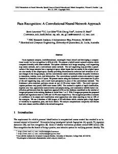
Our face recognition pipeline is similar to the one proposed in [2], but we incorporate a more sophisticated illumination normalization step [24]. Figure (1) summarizes its operation, given by the following main steps: 1. Crop the face region and align the face by mapping the eyes to a canonical location with a similarity transform. 2. Normalize illumination with Tan and Triggs’ [24] Difference of Gaussians (DoG) filter.

Face Recognition with Decision Tree-based Local Binary Patterns 1. Input

2. Crop & Align

3. Normalize

4. Extract features

3

5. Nearest Neighbor match

... Probe

DTLBP

...

Gallery

Fig. 1. Our face recognition pipeline.

3. Partition the face image in a grid with equally sized cells, the size of which is a parameter. 4. For each grid cell, apply a feature extraction operator (such as LBPs) to each pixel in the grid cell. Afterward, create a histogram of the feature values and concatenate these histograms into a single vector, usually known as “spatial histogram”. 5. Classify a probe face with the identity of the nearest neighbor in the gallery, where the nearest neighbor distance is calculated with the (possibly weighted) L1 distance between the histograms of the corresponding face images.

3

Our Approach: Decision Tree Local Binary Patterns

The simple observation behind DT-LBP is that the operation of a LBP over a given neighborhood is equivalent to the application of a fixed binary decision tree. In effect, the aforementioned histograms of LBPs may be seen as quantizing each pair (c, n) with a specially constructed binary decision tree, where each possible branch of the tree encodes a particular LBP. The tree has S levels, where all the nodes at a generic level l compare the center pixel c with a given neighbor nl ∈ n. In this way, at each level l − 1, the decision is such that, if c < nl the vector is assigned to the left node; otherwise, it is assigned to the right node. Since the tree is complete, at level 0 we have 2S leaf nodes. Each of these nodes corresponds to one of the 2S possible LBPs. In fact, seen as a binary number, each LBP encodes the path taken by (c, n) through the tree; for example, in a LBP with S = 8, 11111101 corresponds to a (c, n) pair which has taken the left path at level l = 1 and taken the right path at all other levels. The previous equivalence suggests the possibility of using standard decision tree induction algorithms in place of a fixed tree to learn discriminative LBPlike descriptors from training data. We call this approach Decision Tree Local Binary Patterns or DT-LBP. As a major advantage, by using training data to learn the structure of the tree, DT-LBP can effectively build an adaptive tree, whose main branches are specially tuned to encode discriminative patterns for

4

´ Daniel Maturana, Domingo Mery and Alvaro Soto

Fig. 2. The LBP operator versus the DT-LBP operator.

the relevant target classes. Furthermore, the existence of efficient algorithms to train a decision tree allows DT-LBP to explore larger neighborhoods, such that, at the end of the process the resulting structure of the tree and corresponding pixel comparisons at each node provide more discriminative spatial histograms. Figure 2 compares the operation of regular LBPs with respect to DT-LBPs. After a decision tree is trained, DT-LBP assigns to each leaf node a code given by the path or branch that leads to that node in the tree. In this way, for any input pixel c and the corresponding neighborhood n used to build the tree, the pair (c, n) moves down the tree according to the c < nl comparisons. Once it reaches a leaf node, the respective code is assigned to the center pixel c (code number 1 in Figure 2). As with ordinary LBPs, the DT-LBPs obtained for a given image can be used for classification by building histograms. In summary the proposed approach has the following advantages: – We can obtain adaptive and discriminative LBPs by leveraging well known decision tree construction algorithms (e.g. [21]), as well as more recent randomized tree construction algorithms that have been shown to be very effective in computer vision applications (e.g. [18]). – Since we expect different patterns to be discriminative in different face image regions, we can learn a different tree for each region. – Instead of neighborhood of eight or sixteen pixels as in regular LPBs, we can use a much larger neighborhood and let the tree construction algorithm decide which neighbors are more relevant. – Apart from the feature extraction step, DT-LBP can be used with no modification in any of the many applications where LBP is currently applied.

Face Recognition with Decision Tree-based Local Binary Patterns

3.1

5

Tree Learning Details

To maximize the adaptivity of our algorithm we learn a tree for each grid cell. The trees are recursively built top-down with a simple algorithm based on Quinlan’s classic ID3 method [21]. The algorithm takes as input a “dataset” X = {(ci , ni , yi )}N i=1 , a set of tuples where ci is the value of the center pixel, ni = (ni1 , . . . , nis ) is the vector of values of ci ’s neighbors, and yi is the label of the image from which ci is taken. These values are taken from the pixels in each grid cell of the images in the training data. The following pseudocode summarizes the algorithm: build tree(X ) ≡ {Recursively build DT-LBP tree} if terminate then return LeafNode else m ← choose split(X ) left ← build tree({(ci , ni , yi ) ∈ X | ci ≥ nim }) right ← build tree({(ci , ni , yi ) ∈ X | ci < nim }) return SplitNode(m, left, right) end if choose split(X ) ≡ {Choose most informative pixel comparison} for d = 1 to S do XL ← {(ci , ni , yi ) ∈ X | ci ≥ nid } XR ← {(ci , ni , yi ) ∈ X | ci < nid } |XR | L| ∆Hd ← H(X ) − |X |X | H(XL ) − |X | H(XR ) end for return arg maxd ∆Hd P where H(X ) is the class entropy impurity of X , i.e. H(X ) = − ω p(ω) lg p(ω), p(ω) being the fraction of tuples in X with class label yi = ω. Intuitively, choose split chooses a pixel comparison for a node based on how well this comparison separates tuples from different classes. terminate yields true if a maximum depth is reached, |X | is smaller than a size threshold, or there are no informative pixel comparisons available1 . The size threshold for |X | is fixed as 10, and the maximum depth is a parameter. We define the neighborhood n used by DT-LBP somewhat differently than LBPs. We use a square neighborhood centered around c, and instead of samples taken along a circle, as in regular LBPs, we consider all pixels inside the square as part of the neighborhood (fig. (3)). All the pixels within this square are considered as potential split candidates. The idea is to let the tree construction algorithm find the most discriminative pixel comparisons. The main parameters of this algorithm are the size of the neighborhood n to explore, and the maximum depth of the trees. As shown in Figure 3, the 1

Once a pixel comparison is chosen for a tree node, it provides no information for the descendants of the node. In practice this is used to speed up training.

6

´ Daniel Maturana, Domingo Mery and Alvaro Soto

c

r

Fig. 3. Pixel neighborhood used in DT-LBP. The inner square is the center pixel c, and the neighborhood corresponds to all the pixels enclosed in the larger square. The size of the neighborhood is determined by the radius r.

first parameter is determined by a radius r. The second parameter, tree depth, determines the size of the resulting histograms. Smaller histograms are desirable for space and time efficiency, but as we will show in our experiments, there is a trade-off in accuracy with respect to larger histograms. Using trees opens up various possibilities. We have explored some extensions to the basic idea, such as using a forest of randomized trees (as in [23] and [18]), trees splitting based on a linear combinations of the values of the neighborhood (i.e. nodes split on nT w < c, similarly to [7]), or using ternary trees where a middle branch corresponds to pairs for which |c − ni | <  for a small . This last approach can be considered as the tree-based version of the local ternary patterns described in [24]. So far, we have found that a single tree built with an ID3-style algorithm is the best performing solution.

4

Related work

Our algorithm can be seen as a way to quantize (c, n) pairs using a codebook where each code corresponds to a leaf node. This links our algorithm to various other works in vision that use codebooks of image features to describe the images. Forests of randomized trees have become a popular option to construct codebooks for computer vision tasks. Moosmann et al [18] use Extremely Randomized Clustering forests to create codebooks of SIFT descriptors [15]). Shotton et al. [23] use random forests to create codebooks for use as features in image segmentation. While the use of trees in these works is similar to ours, they use the results of the quantization in a very different way; the features are given to classifiers such as SVMs, which are not suitable for use in our problem. Furthermore, we have found that for our problem single trees are more effective than random forests. Wright and Hua [26] use unsupervised random forests to quantize SIFTlike descriptors for face recognition. The main difference with our algorithm, besides the use of forests versus single trees, is that we do not quantize complex descriptors extracted from the image but work directly on the image itself. In addition, their trees use decision planes as opposed to simple pixel comparisons, which are faster.

Face Recognition with Decision Tree-based Local Binary Patterns

7

There are various recent works using K-Means to construct codebooks to be used for face recognition in a framework similar to ours. Ahonen et al [1] proposed to view the difference c − ni of each neighbor pixel ni with the center as the approximate response of a derivative filter centered on c. Under this view, the LBP operator is a coarse way to quantize the joint responses of various filters (one for each neighbor ni ). Likewise, DT-LBP is also a quantizer of these joint responses, but it is built adaptively and discriminatively. Ahonen tested the K-Means algorithm as an adaptive quantizer, but did not find it to be clearly superior to LBPs for a face recognition task. Meng et al [16] use K-Means to directly quantize patches from the grayscale image. Xie et al [27, 28], as well as [12] use it to quantize patches from images convolved with Gabor wavelets at various scales and orientations. These algorithms are the closest in spirit to our work, since they are partly inspired by LBPs. These algorithms differ from ours in the algorithm used to construct the codebook. They use K-Means, which has the drawback of not being supervised and thus unable to take advantage of labeled data. In addition, trees are more efficient; the time required to quantize a patch with K-Means increases linearly with the size of the codebook, whereas with trees it increases logarithmically. Finally, unlike ours, various of the above algorithms use a bank of Gabor wavelet filters. The convolution of each image with the filter bank adds substantial processing time.

5

Experiments

We perform experiments on the FERET [20] and the CAS-PEAL-R1 [10] benchmark datasets. First, we examine the effects of the two main parameters of DTLBP: the radius r and the maximum tree depth d. In this case, we measure the accuracy of the algorithm on a subset of FERET. Afterward, we report the accuracy of our algorithm on various standard subsets of FERET and CAS-PEAL-R1 with a selected set of parameters. In all images we partition the image into an 7 × 7 grid, as in [2]. While in general we have found this partition to provide good results, it is possible that adjusting the grid size to each dataset may yield better results. For each experiment we show our results along with results from similar works in the recent literature: the original LBP algorithm from Ahonen [2]; the Local Gabor Binary Pattern (LGBP) algorithm, which applies LBP to Gabor-filtered images; the Local Visual Primitive (LVP) algorithm of Meng et al [16], which uses K-Means to quantize grayscale patches; the Local Gabor Textons (LGT) algorithm and the Learned Local Gabor Pattern (LLGP) algorithms, which use K-Means to quantize Gabor filtered-images; and the Histogram of Gabor Phase Patterns (HGPP) algorithms, which quantizes Gabor filtered images into histograms that encode not only the magnitude, but also the phase information from the image. The results are not strictly comparable, since there may be differences in preprocessing and other details, but they provide a meaningful reference. It is worth noting that for each of the algorithm we only show non-weighted variants,

8

´ Daniel Maturana, Domingo Mery and Alvaro Soto

radius

100

Accuracy

98

●

●

●

● ●

●

96 94

3

●

4

●

5

●

6

●

7

92 5

6

7

8

9

10

11

12

13

8

Tree depth Fig. 4. Effect on accuracy of radius and maximum tree depth in FERET fb.

since our algorithm does not currently incorporate weights for different facial regions. 5.1

Effect of Tree Depth and Neighborhood Size

Figure 4 shows the accuracy obtained on FERET fb with various combinations of neighborhood sizes and depths. While neighborhood sizes of r = 1 and r = 2 were also tested, as expected these perform poorly with large trees and are not shown. We see that larger trees tend to boost performance, however, for some radii there is a point where larger trees decrease accuracy. This suggests that overfitting may be occurring for these radii sizes. We also see that while larger radii tend to perform better, all radii larger than 6 perform similarly. Therefore we set the radius to 7 pixels in the following two experiments. 5.2

Results on FERET

For FERET, we use fa as gallery and fb, fc, dup1 and dup2 as probe sets. For training, we use the FERET standard training set of 762 images from the training CD provided by the CSU Face Identification Evaluation System package [6]. We can see that our algorithm relies on the Tan-Triggs normalization step to obtain competitive results on the probe sets with heavy illumination variation. When the normalization step is included, our algorithm obtains the best results on all the probe sets. We argue that the DoG filter in the Tan-Triggs normalization plays a similar role to the Gabor filters in the Gabor-based algorithms, but is much more efficient computationally. 5.3

Results on CAS-PEAL-R1

In the Expression probe set, which does not have intense illumination variation, DT-LBP without illumination normalization obtained the best results, and DTLBP with normalization the second best. The algorithm with normalization

Face Recognition with Decision Tree-based Local Binary Patterns

9

Table 1. Accuracy on FERET probe sets. DT-LBPrd corresponds to a tree of maximum depth d and radius r. TT indicates Tan-Triggs DoG normalization. Accuracies for algorithms other than DT-LBP come from the cited papers. Method LBP [2] LGBP [30] LVP [28] LGT [12] HGPP [29] LLGP [28] DT-LBP78 , no TT DT-LBP710 , no TT DT-LBP712 , no TT DT-LBP78 DT-LBP710 DT-LBP712 DT-LBP713

fb

fc dup1 dup2

0.93 0.51 0.94 0.97 0.97 0.70 0.97 0.90 0.98 0.99 0.97 0.97 0.98 0.44 0.98 0.55 0.99 0.63 0.98 0.99 0.99 0.99 0.99 1.00 0.99 1.00

0.61 0.68 0.66 0.71 0.78 0.75 0.63 0.65 0.67 0.79 0.83 0.84 0.84

0.50 0.53 0.50 0.67 0.76 0.71 0.42 0.47 0.48 0.78 0.78 0.79 0.80

obtains the best result, along with HGPP, in the Accessory probe set. On the lighting dataset, the overall performance of all the algorithms is rather poor. In this case, the best results are given by LGBP, HGPP and LLGP. All these algorithms use features based on Gabor wavelets, which suggests that Gabor features provide more robustness against the extreme lighting variations in this dataset than the DoG filter.

5.4

Discussion

The results show that DT-LBPs are highly discriminative features. Their discriminativity increases as the trees grow, but this has an exponential impact in the computational time and storage cost of using these features . For example, a tree of maximum depth 8 corresponds to a maximum of 256 histogram bins, while a tree with maximum depth 14 corresponds to a maximum of 16384 bins. Since we use 7 × 7 = 49 grid cells, the total number of histogram bins in each spatial histogram is around 802,816 bins. In practice, we find that our C++ implementation is fast enough for many applications – converting an image to a DT-LBP spatial histogram and finding its nearest neighbor in a gallery with more than a thousand images takes a couple of seconds. However, the cost in terms of memory and storage becomes an obstacle to the use of larger trees. For example, a gallery of 1196 subjects with 49 grid cells and trees of maximum depth 14 takes about 3.5 GB of storage when stored naively. However, the resulting dataset is very sparse, which can be taken advantage of to compress it. A straightforward solution is not to use in our coding all the branches of the

10

´ Daniel Maturana, Domingo Mery and Alvaro Soto

Table 2. Accuracy on CAS-PEAL-R1 probe sets. DT-LBPrd corresponds to a tree of maximum depth d and radius r. TT indicates Tan-Triggs DoG normalization. Accuracies for algorithms other than DT-LBP come from the cited papers. Method LGBP [30] LVP [16] HGPP [29] LLGP [28] DT-LBP78 , no TT DT-LBP710 , no TT DT-LBP712 , no TT DT-LBP78 DT-LBP710 DT-LBP712 DT-LBP713

Expression Accessory Lighting 0.95 0.96 0.96 0.96 0.96 0.99 0.99 0.95 0.98 0.98 0.98

0.87 0.86 0.92 0.90 0.80 0.87 0.88 0.89 0.91 0.92 0.92

0.51 0.29 0.62 0.52 0.20 0.23 0.25 0.36 0.39 0.40 0.41

resulting trees but only the most popular ones. This is a similar simplification to the one used by traditional LBPs through the so-called uniform patterns.

6

Conclusions and future work

We have proposed a novel method that uses training data to create discriminative LBP-like descriptors by using decision trees. The algorithm obtains encouraging results on standard datasets, and presents better results that several state-of-theart alternative solutions. In particular, with respect to a face recognizer based on the widely used LBPs, our approach presents a significant increase in accuracy, demonstrating the advantages of using an adaptive and discriminative set of local binary patterns. As future work, our current implementation does not assign different weights to different face regions in the nearest neighbor classification phase. Incorporating weights has been shown to be an effective strategy in various similar works, such as [1] and [28], so we plan to incorporate weights. Furthermore, we are currently working on reducing the size of the resulting histograms while maintaining or improving accuracy. To achieve this we are exploring different methods to learn the decision trees as well as other data structures to represent adaptable LBP-like descriptors. Finally, seeing the good performance of algorithms that use features based on Gabor-filtered images (such as [28] and [29]) we are incorporating these type of features into our algorithm. Acknowledgements. This work was partially funded by FONDECYT grant 1095140 and LACCIR Virtual Institute grant No. R1208LAC005 (http://www. laccir.org). The authors thank Pontificia Universidad Cat´olica de Chile for the VRI Grant and Pontificia Universidad Cat´olica’s School of Engineering for

Face Recognition with Decision Tree-based Local Binary Patterns

11

the FIA Grant. Portions of the research in this paper use the FERET database of facial images collected under the FERET program. The research in this paper uses the CAS-PEAL-R1 face database collected under the sponsorship of the Chinese National Hi-Tech Program and ISVISION Tech. Co. Ltd. Finally, the authors thank the anonymous reviewers for their helpful comments.

References 1. Ahonen, T., Pietik¨ ainen, M.: Image description using joint distribution of filter bank responses. Pattern Recognition Letters 30 (2009) 368–376 2. Ahonen, T., Hadid, A., Pietik¨ ainen, M.: Face description with local binary patterns: Application to face recognition. IEEE Transactions on Pattern Analysis and Machine Intelligence 28 (2006) 2037–2041 3. Albiol, A., Monzo, D., Martin, A., Sastre, J., Albiol, A.: Face recognition using HOG-EBGM. Pattern Recognition Letters 29 (2008) 1537–1543 4. Bay, H., Ess, A., Tuytelaars, T., Gool, L.V.: Speeded-Up Robust Features (SURF). Computer Vision and Image Understanding 110 (2008) 346–359 5. Bicego, M., Lagorio, A., Grosso, E., Tistarelli, M.: On the use of SIFT features for face authentication. In: CVPR. (2006) 6. Bolme, D.S., Beveridge, J.R., Teixeira, M., Draper, B.A.: The CSU face identification evaluation system: Its purpose, features and structure. In: ICCV. (2003) 7. Bosch, A., Zisserman, A., Munoz, X.: Image classification using random forests and ferns. In: ICCV. (2007) 8. Dalal, N., Triggs, B.: Histograms of oriented gradients for human detection. In: CVPR. (2005) 9. Dreuw, P., Steingrube, P., Hanselmann, H., Ney, H.: SURF-face: Face recognition under viewpoint consistency constraints. In: BMVC. (2009) 10. Gao, W., Cao, B., Shan, S., Chen, X., Zhou, D., Zhang, X., Zhao, D.: The CASPEAL large-scale chinese face database and baseline evaluations. IEEE Transactions on System Man, and Cybernetics (Part A) 38 (2008) 149–161 11. Heikkil¨ a, M., Pietik¨ ainen, M., Schmid, C.: Description of interest regions with local binary patterns. Pattern Recognition 42 (2009) 425–436 12. Lei, Z., Li, S., Chu, R., Zhu, X.: Face recognition with local Gabor textons. Advances in Biometrics (2007) 49–57 13. Liao, S., Chung, A.C.S.: Face recognition by using elongated local binary patterns with average maximum distance gradient magnitude. In: ACCV. (2007) 672–679 14. Liao, S., Zhu, X., Lei, Z., Zhang, L., Li, S.: Learning multi-scale block local binary patterns for face recognition. In: Advances in Biometrics. (2007) 828–837 15. Lowe, D.G.: Distinctive image features from scale-invariant keypoints. International Journal of Computer Vision 60 (2004) 91–110 16. Meng, X., Shan, S., Chen, X., Gao, W.: Local Visual Primitives (LVP) for face modelling and recognition. In: ICPR. (2006) 17. Mikolajczyk, K., Schmid, C.: Performance evaluation of local descriptors. IEEE Transactions on Pattern Analysis and Machine Intelligence 27 (2005) 1615–1630 18. Moosmann, F., Nowak, E., Jurie, F.: Randomized clustering forests for image classification. IEEE Transactions on Pattern Analysis and Machine Intelligence 30 (2008) 1632–1646 19. Ojala, T., Pietik¨ ainen, M., Harwood, D.: A comparative study of texture measures with classification based on featured distributions. Pattern Recognition 29 (1996) 51–59

12

´ Daniel Maturana, Domingo Mery and Alvaro Soto

20. Phillips, P.J., Moon, H., Rizvi, S.A., Rauss, P.J.: The FERET evaluation methodology for Face-Recognition algorithms. IEEE Transactions on Pattern Analysis and Machine Intelligence 22 (2000) 1090–1104 21. Quinlan, J.R.: Induction of decision trees. Machine Learning 1 (1986) 81–106 22. Ruiz-del-Solar, J., Verschae, R., Correa, M.: Recognition of faces in unconstrained environments: A comparative study. EURASIP Journal on Advances in Signal Processing 2009 (2009) 1–20 23. Shotton, J., Johnson, M., Cipolla, R.: Semantic texton forests for image categorization and segmentation. In: CVPR. (2008) 24. Tan, X., Triggs, B.: Enhanced local texture feature sets for face recognition under difficult lighting conditions. IEEE Transactions on Image Processing 19 (2010) 1635–50 25. Wolf, L., Hassner, T., Taigman, Y.: Descriptor based methods in the wild. In: Real-Life Images Workshop at ECCV. (2008) 26. Wright, J., Hua, G.: Implicit elastic matching with random projections for posevariant face recognition. In: CVPR. (2009) 1502–1509 27. Xie, S., Shan, S., Chen, X., Gao, W.: V-LGBP: Volume based Local Gabor Binary Patterns for face representation and recognition. In: ICPR. (2008) 28. Xie, S., Shan, S., Chen, X., Meng, X., Gao, W.: Learned local Gabor patterns for face representation and recognition. Signal Processing 89 (2009) 2333–2344 29. Zhang, B., Shan, S., Chen, X., Gao, W.: Histogram of Gabor phase patterns (HGPP): A novel object representation approach for face recognition. IEEE Transactions on Image Processing 16 (2007) 57–68 30. Zhang, W., Shan, S., Gao, W., Chen, X., Zhang, H.: Local Gabor Binary Pattern Histogram Sequence (LGBPHS): A novel non-statistical model for face representation and recognition. In: ICCV. (2005) 31. Zou, J., Ji, Q., Nagy, G.: A comparative study of local matching approach for face recognition. IEEE Transactions on Image Processing 16 (2007) 2617–2628