SVD to approximate a matrix that is rank 3 in a noise- ... quence. In [1], the 3D positions of the feature points ... to compute the rank 1 matrix that best matches the ... 3D Shape The shape of the rigid object is a para- ... matrix that determine the orientation of the o.c.s. rel- ..... (the left side vertical face of the box in the frames of.
IEEE Signal Processing Society International Conference on Image Processing October 1999, Kobe, Japan c 1999 IEEE
A Fast Algorithm for Rigid Structure from Image Sequences Pedro M. Q. Aguiar
∗
Jos´e M. F. Moura
Department of Electrical and Computer Engineering Carnegie Mellon University, Pittsburgh PA, USA {aguiar,moura}@ece.cmu.edu Abstract The factorization method [1] is a feature-based approach to recover 3D rigid structure from motion. In [2], we extended their framework to recover a parametric description of the 3D shape. In [1, 2], the 3D shape and 3D motion are computed by using an SVD to approximate a matrix that is rank 3 in a noiseless situation. In this paper, we develop a new algorithm that has two relevant advantages over the algorithms of [1, 2]. First, instead of imposing a common origin for the parametric representation of the 3D surface patches, as in [2], we allow the specification of different origins for different patches. This improves the numerical stability of the image motion estimation algorithm and the accuracy of the 3D structure recovery algorithm. Second, we show how to compute the 3D shape and 3D motion by a simple factorization of a modified matrix that is rank 1 in a noiseless situation, instead of a rank 3 matrix as in [1, 2]. This allows the use of very fast algorithms even when using a large number of features (or regions) and large number of frames.
1
Introduction
The factorization method [1] is an elegant method to recover 3D rigid structure from an image sequence. In [1], the 3D positions of the feature points are expressed in terms of cartesian coordinates in a world-centered coordinate system, and the images are modeled as orthographic projections. The 2D projection of each feature point is tracked along the image sequence. The 3D shape and motion are then estimated by factorizing a measurement matrix whose entries are the set of trajectories of the feature point projections. The factorization of the measurement matrix, which is rank 3 in a noiseless situation, is computed by using the Singular Value Decomposition (SVD). The factorization method was extended to ∗ The
first author is also affiliated with ISR-IST, Lisboa, Portugal. The first author was partially supported by INVOTAN.
the scaled-orthography and the paraperspective projections in [3]. When the goal is the recovery of a dense representation of the 3D shape, the factorization approach of [1, 3] may not solve the problem satisfactorily because of two drawbacks. First, being feature-based, it would be necessary to track a huge number of features to obtain a dense description of the 3D shape. This is usually impossible because only distinguished points, as brightness corners, can by accurately tracked. Second, even if it is possible to track a large number of features, the computational cost of the SVD involved in the factorization of the measurement matrix would be very high. These drawbacks motivated the extension of the factorization approach to recover a parametric description of the 3D shape, as we did in [2]. Instead of tracking pointwise features, we track regions for which the motion induced on the image plane is described by a single set of parameters. In this paper, we reformulate the problem. The reformulation leads to a new algorithm that has two relevant advantages over the algorithms of [1, 2]. First, instead of imposing a common origin for the parametric representation of the 3D surface patches, as in [2], we allow the specification of different origins for different patches. This improves the numerical stability of the image motion estimation algorithm and the accuracy of the 3D structure recovery algorithm, as will become clear later. Second, we show how to compute the 3D shape and 3D motion by a simple factorization of a modified matrix that is rank 1 in a noiseless situation, instead of a rank 3 matrix as in [1, 2]. This simplifies the decomposition and normalization stages involved in the factorization approach. We avoid the computation of the SVD by using a fast iterative method to compute the rank 1 matrix that best matches the data. Reference [4] compares the computational cost of the rank 1 factorization with the computational cost of the original rank 3 factorization method [1] for the feature-based case.
Paper Overview Section 2 describes the scenario. In section 3, we characterize the motion induced in the image plane. Sections 4 and 5 deal with the recovery of the 3D struacture from the image motion. In section 6, we detail a real video experiment. Section 7 concludes the paper.
the coordinates of the origin of the o.c.s. with respect to the c.c.s. (3D translation), and Θf is the rotation matrix that determine the orientation of the o.c.s. relative to the c.c.s. (3D rotation). A point with coordinates [x, y, z]T in the o.c.s. has the following coordinates in the c.c.s., at frame f ,
2
iz f tuf x j z f y + tv f , twf z kz f (3) where the matrix above is the 3D rotation matrix Θf .
Scenario
We consider a rigid body moving in front of the camera. We attach coordinate systems to the object and to the camera. The object coordinate system (o.c.s.) has axes labeled by x, y, and z. The camera coordinate system (c.c.s.) has axes labeled by u, v, and w. We consider that the o.c.s. coincides with the c.c.s. on the first frame. The image plane is defined by the axes u and v. The images are modeled as orthographic projections of the object texture. Our algorithm is easily extended to the scaled-orthography and the paraperspective projections by proceeding as [3] does for the original factorization method. 3D Shape The shape of the rigid object is a parametric description of the object surface. Although our approach is general enough to cope with general parameterizations, we consider in this paper objects whose shape is given by a piecewise planar surface �with K patches. The shape parameter vector is a = ak00 , ak10 , ak01 , 1 ≤ k ≤ K where z = ak00 + ak10 (x − xk0 ) + ak01 (y − y0k )
(1)
describes the shape of the patch k in the o.c.s.. In what respects to the representation of the planar patches, the parameters xk0 and y0k can have any value, for example they can be made zero as we did in [2]. In this paper, we allow the specification of general parameters xk0 , y0k . The relevance of this generalization is obvious: the shape of a small patch k with support region {(x, y)} located far from the the point (xk0 , y0k ) has an high sensibility with respect to the shape parameters ak10 and ak01 . To minimize this sensibility, we choose for (xk0 , y0k ) the centroid of the support region of patch k. With this choice, we improve the numerical stability of the image motion estimation algorithm and the accuracy of the 3D structure recovery algorithm. To simplify the notation, we define the vectors ak = [ak10 , ak01 ]T , s = [x, y]T , and sk0 = [xk0 , y0k ]T , and rewrite the shape of the patch k as z = ak00 + aTk (s − sTk0 ).
(2)
3D Motion We define the 3D motion of the object by specifying the position of the�o.c.s. relative to the c.c.s. � in terms of tuf , tv f , tw f , Θf where tuf , tv f , tw f are
ixf uf vf = j x f wf kxf
3
iy f jy f ky f
Image Motion
In this section we show that the motion induced in the image plane by the body-camera 3D motion is affine with different parameterizations for regions corresponding to different patches. We relate the parameters of the affine motion model to the 3D shape and 3D motion parameters. Under orthography, the point with coordinates (x, y, z) in the o.c.s. projects in frame f to the image point (uf , vf ) given by � � x uf = M f y + tf , (4) vf z where M f collects the first and second rows of the 3D rotation matrix introduced in expression (3) and tf = [tuf , tv f ]T . Consider a generic point in the object surface with coordinates s = [x, y]T and z given by expression (2). We denote by uf (s) = [uf (s), vf (s)]T the trajectory of the projection of the point s in the image plane. Since we have chosen the coordinate systems to coincide on the first frame, we have u1 (s) = s. At frame f , the point s projects according to expression (4), to the image point uf (s) = N f s + nf z + tf ,
(5)
where we have decomposed the matrix M f as M f = [N f , nf ] where N f collects the first and second columns of M f and nf is the third column of M f . Affine Motion Model By inserting expression (2) into expression (5), we express the image displacement between frame 1 and frame f in terms of the 3D shape and 3D motion parameters, for the points s that fall into patch k of the object surface. After simple manipulations, we obtain ukf (s) = (N f + nf aTk )(s − sk0 ) + N f sk0 + nf ak00 + tf . (6)
Denoting the matrix that multiplies (s − sk0 ) and the vector corresponding to the term independent of s by � k D f = N f + nf aTk , (7) dkf = N f sk0 + nf ak00 + tf
To eliminate the dependence of the image motion parameters on the translation, we replace the translation estimates into expression (7) and define a new set ˜ k } related to {dk } by of parameters {d f
K X ˜ k = dk − 1 dlf . d f f K
we rewrite expression (6) as ukf (s)
=
DK f (s
−
sk0 )
+
dkf .
4
Rigid Structure from Motion
The problem of inferring 3D rigid structure from the image motion is formulated as estimating the 3D motion parameters {N f , nf , tf , 2 ≤ f ≤ F } and the 3D shape parameters {ak00 , ak , 1 ≤ k ≤ K} from the image motion parameters {D kf , dkf , 2 ≤ f ≤ F, 1 ≤ k ≤ K} by inverting the overconstrained set of equations of expression (7). We start by estimating the translation. By choosing the coordinate system in such a way P object k a = 0 and the image origin in such that k 00 P k T s a way that k 0 = [0, 0] , we obtain the Least Squares (LS) estimate for the translation vector tf as the mean of the vectors {dkf , 1 ≤ k ≤ K}, K X ˆtf = 1 dkf . K k=1
(9)
(10)
l=1
(8)
Expression (8) shows that the image coordinates at frame f , uf , of the the points belonging to the object surface are affine mappings of their image coordinates frame 1, u1 = s. Expression (7) relates the coefficients of the affine motion models for each patch k to the 3D motion parameters and the 3D shape parameters corresponding to patch k. Image Motion Estimation Except for particular 3D motions, the image motion corresponding to different surface patches is described by different affine parameterizations. The problem of estimating the support regions of the surface patches leads to the segmentation of the image motion field. The segmentation according to image motion has been widely addressed in the past, see for example [5, 6]. We use the simple method of sliding a rectangular window across the image and detect abrupt changes in the affine motion parameters. Another possible way to use our structure from motion approach is to select a priori the support regions of the surface patches. In fact, our framework is general enough to accommodate the feature tracking approach because it corresponds to selecting a priori a set of small (pointwise) support regions with shape described by z = constant in each region. In reference [4] we exploit the feature-based approach.
f
Defining the matrices Rkf and S Tk as � i h I2×2 T ˜k and S = Rkf = D kf d k f aTk
sk0 ak00
�
,
(11) we rewrite the equation system (7) in matrix format as Rkf = M f S Tk .
(12)
Expression (12) relates the image motion parameters at frame f and patch k to the 3D rotation at frame f and the 3D shape parameters for the patch k. To make explicit the entire set of equations that arise from considering every patch 1 ≤ k ≤ K and every frame 2 ≤ f ≤ F , we define the 2(F − 1) × 3K matrix R of image motion parameters, the 2(F −1)×3 matrix M of 3D rotation parameters, and the 3K × 3 matrix S of 3D shape parameters as 1 S1 M2 R2 · · · RK 2 .. , M = .. , S = .. , .. R = ... . . . . R1F
RK F
SK (13) and we write the relation between the image motion parameters and the 3D structure parameters as ···
MF
R = M ST .
(14)
The matrix R of image motion parameters is highly rank deficient. In a noiseless situation, R is rank 3 reflecting the high redundancy in the data, due to the rigidity of the object.
5
Rank 1 Factorization
Estimating the 3D shape and 3D rotation parameters given the observation matrix R is a nonlinear LS problem. The factorization approach [1, 2] finds a suboptimal solution to this problem in two stages. The first stage, decomposition stage, solves R = M S T in the LS sense by computing the SVD of the matrix R and selecting the 3 largest singular values. 1 From R ' U ΣV T , the solution is M = U Σ 2 A and 1 S T = A−1 Σ 2 V T where A is a non-singular 3 × 3 matrix. The second stage, normalization stage, computes A by approximating the constraints imposed by the structure of the matrices M and S.
The formulation we adopt in this paper takes advantage of the fact that the first two rows of S T are known. The problem is then reduced to, given R, compute M and {akmn }. We also perform in sequence the decomposition and normalization stages. These stages are as follows. For more details see [4]. Decomposition Because the first two rows of S T are known (see expressions (11), and (13)), we show that the unconstrained bilinear problem R = M S T is solved by the factorization of a rank 1 matrix, rather than a rank 3 matrix like in [1, 2]. Define M = [M 0 , m3 ] and S = [S 0 , a]. Matrices M 0 and S 0 contain the first two columns of M and S, respectively, m3 is the third column of M , and a is the third column of S. We decompose the shape parameter vector a into the component that belongs to the space spanned by the columns of S 0 and the component orthogonal to this space as a = S 0 b + a1 , with aT1 S 0 = [0, 0]. Using these definitions, we rewrite R as R = M 0 S T0 + m3 bT S T0 + m3 aT1 .
(15)
The decomposition stage is formulated as
min
R − M 0 S T0 − m3 bT S T0 − m3 aT1 , F M 0 ,m3 ,b,a1 (16) where k.kF denotes the Frobenius norm. By solving the linear LS for M 0 in terms of the other variables, we get �−1 � c 0 = RS 0 S T S 0 − m 3 bT , (17) M 0
where we used the orthogonality between a1 and S 0 . c 0 in (16), we get By replacing M
e (18) − m3 aT1 , min R m3 ,a1 F � � �−1 � T e = R I − S0 ST S0 (19) S where R 0 0 .
We see that the decomposition stage does not determine the vector b. This is because the component of a that lives in the space spanned by the columns of S 0 does not affect the space spanned by the columns of the entire matrix S and the decomposition stage restricts only this last space. The solution for m3 and a1 is given by the rank 1 e In a noiseless situamatrix that best approximates R. e e tion, R is rank 1 (we get R = m3 aT1 by replacing (15) e in (19)). By computing the largest singular value of R and the associated singular vectors, we get e ' uσv T , R
c3 = αu, m
ˆ T1 = a
σ T v , α
(20)
where α is a normalizing scalar different from 0. To compute u, σ, and v we use a fast algorithm outlined in [4]. This makes our decomposition stage simpler e in (19) is R multhan the one in [1, 2]. In fact, R tiplied by the orthogonal projector onto the orthogonal complement of the space spanned by the columns of S 0 . This projection reduces the rank of the problem e from 3 (matrix R) to 1 (matrix R). Normalization We compute α and b by imposing the constraints that come from the structure of M . By c3 in (17), we get replacing m � � i h I 0 2×2 2×1 c c0 m , (21) M= M ¯ c3 = N −αbT α where
N=
�
�−1 � RS 0 S T0 S 0
u
�
.
(22)
The constrains imposed by the structure of M are the unit norm of each row and the orthogonality between row 2j and row 2j − 1. In terms of N , α, and b, the constraints are � � I 2×2 −αb T ni = 1 and (23) ni −αbT α2 (1 + bT b) nT2j
�
I 2×2 −αbT
−αb α2 (1 + bT b)
�
n2j−1 = 0,
(24)
where nTi denotes the row i of matrix N . We compute α and b from the linear LS solution of the system above in a similar way to the one described in [1]. The normalization stage is also simpler than the one in [1] because the number of unknowns is 3 T (α and b = [b1 , b2 ] ) as opposed to the 9 entries of a generic 3 × 3 normalization matrix.
6
Experiment
We used a hand hold taped video sequence of 30 frames showing a box over a carpet. Figure 1 shows frames 1 and 10 of the video sequence. The 3D shape of the scene is well described in terms of four planar patches. One corresponds to the floor, and the other three correspond to the three visible faces of the box. The camera motion was approximately a rotation around the box. We processed the box video sequence by using the method described above. We start by estimating the affine motion parameters. The plots in figure 2 represent the time evolution of the affine motion parameters. The 6 affine motion parameters are the entries of the 2 × 2 matrix D kf and the 2 × 1 vector dkf , see expression (8). The top four plots of figure 2 represent the entries of D kf as a function of f for each of the four
the rank 1 factorization method. Figure 3 shows two perspective views of the reconstructed 3D shape with the scene texture mapped on it. We see that the angles between the planar patches are correctly recovered.
Figure 1: Frames 1 and 10 of the box video sequence.
planar patches. The bottom two plots represent dkf . We used four different line types to identify each of the planar patches. The solid line corresponds to patch 1 (the left side vertical face of the box in the frames of figure 1). The dotted line corresponds to patch 2 (the right side vertical face of the box). The dash-dotted line corresponds to patch 3 (the top of the box). The dashed line corresponds to patch 4 (the floor). We see the evolution of the set of affine parameters is distinct for each surface patch, in particular see the evolution of D 11 , D 12 , and d1 . 1−,2:,3−.,4−−
1−,2:,3−.,4−−
1.2
0.1
1.15
0.05
D12
0
−0.05
D11
1.1
1.05
1
−0.1
0.95
−0.15
0.9
−0.2
0.85
0
5
10
15
20
25
30
−0.25
f 1−,2:,3−.,4−−
7
Conclusion
We proposed a fast method to recover 3D rigid structure from motion. Rather than relying on the tracking of pointwise features, the image motion estimation step makes use of the affine motion parameterization for larger regions, leading to robust estimates of the image motion parameters. The 3D structure from motion step is robust because it takes into account the rigidity of scene over a set of frames. This step is accomplished with very low computational cost by factorizing a rank 1 matrix. The experimental results illustrate the performance of the method.
References 0
5
10
15
20
25
30
f 1−,2:,3−.,4−− 1.2
0.05
Figure 3: Two perspective views of the reconstructed 3D shape and texture.
[1] Carlo Tomasi and Takeo Kanade. Shape and motion from image streams under orthography: a factorization method. IJCV, 9(2):137–154, 1992.
0.045
1.15
[2] Pedro M. Q. Aguiar and Jos´e M. F. Moura. Video representation via 3D shaped mosaics. In IEEE ICIP, Chicago, USA, October 1998.
0.04
1.1
0.035
0.03
D21
D22
1.05
0.025
1
0.02
0.015
0.95
0.01
0.9 0.005
0
0
5
10
15
20
25
30
0.85
0
5
10
15
20
25
30
f 1−,2:,3−.,4−−
f 1−,2:,3−.,4−−
0
40
[4] Pedro M. Q. Aguiar and Jos´e M. F. Moura. Factorization as a rank 1 problem. In IEEE CVPR, Fort Collins, USA, June 1999.
−1 30
−2 20
−3
−4
d2
d1
10
−5
0
[5] H. Zheng and S. Blostein. Motion-based object segmentation and estimation using the MDL principle. IEEE Trans. Image Processing, 4(9), 1995.
−6 −10
−7 −20
−8
−30
[3] Conrad J. Poelman and Takeo Kanade. A paraperspective factorization method for shape and motion recovery. IEEE PAMI, 19(3):206–218, 1997.
0
5
10
15
f
20
25
30
−9
0
5
10
15
20
25
30
f
Figure 2: Estimates of the image motion parameters. From the affine motion parameters of figure 2, we have recovered the 3D structure of the scene by using
[6] M. M. Chang, A. M. Tekalp, and M. I. Sezan. Simultaneous motion estimation and segmentation. IEEE Trans. Image Processing, 6(9), 1997.