Computational Linguistics and Chinese Language Processing Vol. 11, No. 1, March 2006, pp. 73-86
73
© The Association for Computational Linguistics and Chinese Language Processing
A Fast Framework for the Constrained Mean Trajectory Segment Model by Avoidance of Redundant Computation on Segment1 Yun Tang∗, Wenju Liu∗, Yiyan Zhang+ and Bo Xu∗
Abstract The segment model (SM) is a family of methods that use the segmental distribution rather than frame-based density (e.g. HMM) to represent the underlying characteristics of the observation sequence. It has been proved to be more precise than HMM. However, their high level of complexity prevents these models from being used in practical systems. In this paper, we propose a framework that can reduce the computational complexity of the Constrained Mean Trajectory Segment Model (CMTSM), one type of SM, by fixing the number of regions in a segment so as to share the intermediate computation results. Our work is twofold. First, we compare the complexity of SM with that of HMM and point out the source of the complexity in SM. Secondly, a fast CMTSM framework is proposed, and two examples are used to illustrate this framework. The fast CMTSM achieves a 95.0% string accurate rate in the speaker-independent test on our mandarin digit string data corpus, which is much higher than the performance obtained with HMM-based system. At the mean time, we successfully keep the computation complexity of SM at the same level as that of HMM. Keywords: Speech Recognition, Segment Model, Mandarin Digit String Recognition
1. Introduction The Hidden Markov Model (HMM) [Rabiner et al. 1993] has been used successfully for
1
This work was supported in part by the China National Nature Science Foundation (No. 60172055) and the Beijing Nature Science Foundation (No.4042025). ∗ Institute of Automation, Chinese Academy of Sciences, P.O.Box 2728, nlpr, Beijing 100080 Tel: +086 01062659279 Fax: +086 01062551993 E-mail:
[email protected] + Institute of Scientific and Technical Information of China [Received Feb. 24, 2005; Revised Oct. 8, 2005; Accepted Oct. 12, 2005]
74
Yun Tang et al.
acoustic modeling in many speech recognition systems. Given the state sequence, feature vectors are assumed to be conditionally independent, and the task of extracting the trajectory can be elegantly achieved by applying the Viterbi algorithm frame by frame. However, the above assumption is far from realistic, which limits the HMM’s ability to capture the relations within a segment. Another weakness of HMM is that it is not accurate enough to represent a non-stationary observation sequence by means of a piecewise constant state [Deng et al. 1994; Hon et al. 1999]. In order to handle these problems, a lot of methods have been proposed, including SM [Ostendorf et al. 1996], which is a family of methods among them. SM is totally different from HMM in terms of its segmental decoding method and potential for accomplishing some tasks effectively that are naturally difficult for an HMM based system, since it integrates more segmental information into the decoding process, produces the n-best list during the decoding process etc. However, the good acoustic modeling of SM is at the cost of high computation, which is much higher than that of HMM. It prevents SM from being applied in practical systems. The high complexity of SM is mainly due to the segment evaluation process. Segment evaluation cannot be decomposed and the intermediate computation information is not shareable between different segments even when two segments only differ by one frame. Previous work accelerated SM using efficient segment pruning algorithms. V. Digalakis et al. [1992] proposed a pruning method to speed up SM. They estimate the score of a segment from part of the segment. Then those hypotheses with low likelihood are pruned before the whole segment is evaluated. The amount of reduction in computation depends on the discrimination ability of the feature vector. S. Lee et al. [1998] and J. Glass [2003] proposed a landmark-based algorithm that reduces the search space by detecting the potential boundaries of phonemes with the aid of special features or HMM decoders, so that the number of the possible hypothesized segments in the search space can be reduced greatly. However, since the detection of boundaries is unreliable and not accurate enough, the efficiency of this algorithm is discounted. The most important point is that the speed of SM based on the above methods is still far slower than that of HMM, since the computations performed by these algorithms are based on segments, while in the case of HMM, they are based on frames. In this paper, we propose a framework to reduce the complexity of the Constrained Mean Trajectory Segment Model (CMTSM) [Ostendorf et al. 1996], one family of SM. In this new framework, CMTSM can divide segment computations into frame computations, which are shared between different segments; thus, the redundant computations of segments can be avoided. Guided by this framework, we have measured the complexity of Stochastic Segment Model (SSM) [Ostendorf et al. 1989] based on the number of Gaussian mixture models evaluated during recognition, and found that the complexity is not proportional to the product of the model’s number and the maximum allowable duration, but is only related to the number of models, or more exactly, to the number of regions in the system.
A Fast Framework for the Constrained Mean Trajectory Segment Model by
75
Avoidance of Redundant Computation on Segment The complexity of SSM is on the same level as that of HMM. The speed of the Parametric Trajectory Model (PTM) [Gish et al. 1992; Deng et al. 1994], another type of CMTSM, can also be greatly enhanced with some minor modifications of the original algorithm, based on our framework. The rest of this paper is organized as follows. SM is introduced in the next section by comparing HMM with SM in terms of modeling and decoding. Then, in Section 3, we present the fast framework for CMTSM and two examples, the fast SSM and the fixed PTM, illustrate it. Section 4 presents experimental results obtained with the fast framework. Finally, conclusions are drawn in Section 5.
2. Segment Model and Decoding 2.1 Introduction to the Segment Model In HMM, the model unit is the state, and the relations among feature vectors are represented by the relations among the states mapping to these features. In SM, the model unit is based on segments, such as phonemes, syllables, and words. Hence, the relations between feature vectors in the same segment are modeled directly. The probability density of a variable length feature sequence x1l = {x1 , x2 ,...xl } measured by SM can be represented as follows: p( x1l | α ) = f ( x1l | α ) g ( x1l | α ) ,
(1)
where α is the label of the acoustic model, f ( x1l | α ) is the output density of SM, and g ( x1l | α ) is a segment level score, such as the duration score.
2.2 Decoding Comparison between HMM and SM The goal of a speech recognizer is to find the most likely word sequence given sentence x1T . Let α1N be the label sequence of acoustic models representing words intended by the speaker, who produces x1T above. That is,
αˆ1N = arg maxN p (α1N | x1T ) = arg maxN p(α1N ) p( x1T | α1N ) , N ,α1
N ,α1
(2)
where p(α1N ) is the probability measured by the language model and p( x1T | α1N ) is the density measured by acoustic models. More exactly, p( x1T | α1N ) is the product of acoustic models' densities in different segments of x1T : p( x1T | α1N ) =
N
N
∑ ∏ p( xS (i −1) +1 | α i ) ≈ max ∏ p ( xS (i −1)+1 | α i ) , S (i )
S∈ΛT , N i =1
S (i − 1) < S (i ) , S (0) = 0 and S ( N ) = T ,
S
i =1
S (i )
(3)
76
Yun Tang et al.
where ΛT , N is the segmentation boundary set dividing a T -length sequence into N parts and S (i ) is the boundary point of segment i .
2.2.1 Decoding in HMM The above decoding process is accomplished by the Viterbi algorithm in HMM. We will take a left-to-right HMM without state skipping as an example to illustrate decoding in HMM: * * Jm (α , i ) = ln p ( xm | α , i ) + max ( J m −1 (α , j )). i ≤ m ≤ T , 1 ≤ α ≤| Ω |, 2 ≤ i ≤ Lα , i −1≤ j ≤i
(4)
* where J m (α , i ) is the maximum accumulated score for the state sequence from the 1-th frame to the m -th frame, given state i and model label α for frame xm ; p( xm | α , i ) is the state score of frame xm ; Ω is the number of models; Lα is the number of states for α .
The above formula can be applied to all internal states of each model (i.e., i ≥ 2 ). At the boundary of the model, i.e., i = 1 , the formula is in the following form: * * * Jm (α ,1) = ln p ( xm | α ,1) + max [ J m −1 ( β , Lβ ) + ln( p (α )), J m −1 (α ,1)]. 1≤ β ≤|Ω|
(5)
The final solution for the best path is J * = max[ JT* (α , Lα ] ,
(6)
1≤α ≤ Ω
and the best path can be obtained by backtracking the best final score. The cost of the Viterbi algorithm is essentially the cost of computing the state scores. According to (4) and (5), the amount of computation required for the state scores is proportional to the number of states in each model and the observation sequence length. If the pruning is not considered, the approximate time complexity for the Viterbi algorithm is O(T ⋅ | Ω | ⋅L ⋅ CS ) , where CS is the time cost of computing p( xm | α , i ) and L is the average number of states in each model.
2.2.2 Decoding in SM SMs have to explore all possible segment boundaries due to the segmental decoding, whereas the problem of obtaining exact acoustic model boundaries can be avoided with HMM, since the frame that the exit state maps to is the boundary of the model. Though the decoding procedure can be performed by means of dynamic programming, the complexity of SM is still much higher than that of HMM. The decoding formula for SM is * Jm = max{ Jτ* + ln[ p ( xτm | α )]( m − τ ) + ln[ P (α )] + C },
τ ,α
(7)
A Fast Framework for the Constrained Mean Trajectory Segment Model by
77
Avoidance of Redundant Computation on Segment * is the accumulated score of the best model sequence ending at time point m and C where J m is the insert factor for each segment. The best segment sequence can be obtained by back-tracking from the best final score JT* .
Given the beginning (or end) point of models, the decoder has to hypothesize segments with different durations, from the minimum to the maximum length, to determine the other boundary point of the segment that may spring from this point. Assuming that the maximum allowed duration is Lmax , we find that the time complexity of SM is O(CSeg ⋅ T ⋅ | Ω | ⋅Lmax ) , where CSeg is the time cost of a segment and is comparable with or even more complex than CS ⋅ L in HMM. Hence, SM is more costly than HMM.
3. Fast Framework for CMTSM As discussed in Section 2.2.2, the high complexity of SM is due to two factors. First, SM explores more hypothesized models than HMM does in each frame; second, in each frame, SM needs to measure the densities of segments that pass this point, whereas HMM only needs to evaluate the densities of states mapping to this point. The second factor is more important for current SM systems, since density evaluation represents the lion’s share in the whole computation. Figure 1 shows the percentage of the time spent on density evaluation against the total time needed for the digit string recognition task with HMM and SSM. The model unit for SSM and HMM is the context independent whole-word. The computation involved in density evaluation is extremely time-consuming in the case of the conventional SSM and 97.6% of the time is spent obtaining segment scores, whereas the corresponding percentage in the case of HMM is only 51.4%. The time cost ratio for density evaluation in SM is much higher than that in HMM. The key advantage of our fast framework is that it changes the computation in SM from segment-based style to frame-based style and the frame-based results can be shared by different segments. Such transformation can be achieved in one family of SM, i.e., CMTSM. In the fast SM, which we will describe below, the time cost ratio for density evaluation is lowered to 64.2%, close to that of HMM. The details of experimental setup and total time used for decoding will be given in Section 4 (Table 5). 97. 6%
100% 80%
64. 2% 60%
51. 4%
40% 20% 0% HMM ( Uni phone, Vi t er bi )
SSM
Fas t SSM
Figure 1. Percentage of the time for density evaluation in the decoding
78
Yun Tang et al.
Those SMs, including SSM and PTM, whose segmental distributions are modeled by means of region distributions while frame-based features are assumed to be conditionally independent given the region sequence, are called CMTSM. The so-called region here is similar to the conception of the state in HMM, which is the basic unit used to measure the probability distribution of a frame. The value of f ( x1l | α ) in (1) is the product of a series of frame-based region scores [Ostendorf et al. 1996]: l
ln f ( x1l | α ) = ∑ ln p ( xi | α , ri , l ) ,
(8)
i =1
where p( xi | α , ri , l ) is the score of region ri in frame xi for model α , given duration l . The mapping of a feature vector to a region is only related to the segment duration and its position in the segment. So the measurement of the frame score for a specific region is unrelated to other frames or other regions. The assumption, frame-based features being assumed to be conditionally independent given the region sequence in CMTSM, guarantees to change the density evaluation from segment-based style to frame-based style, and the segment score can be obtained by recombining the region scores in an efficient way. However, these frame-based results can not be shared among different segments, since region models are conditional on the segment duration, as Equation (8) shows. We relax the modeling condition by assuming that the region model is independent of the segment duration. In order to achieve this, we use linear time resampling to map the variable length segment x1l to a fixed length feature sequence ylL , so all the segment models have the same duration. In other words, the duration can be ignored in region models. In this way, the region scores can be shared by segments with different durations. The resampling function is [Ostendorf et al. 1989] yi = x⎢ i ⎥ , 0 ≤ i < L, ⎢ L ⋅l ⎥ ⎣ ⎦
(9)
where ⎢⎣ z ⎥⎦ is the largest integer n ≤ z . Equation (8) can be simplified as L
ln f ( x1l | α ) = ∑ ln p ( yi | α , ri ) .
(10)
i =1
In short, to speed up CMTSM, we first resample a variable length segment to obtain a fixed length sequence and then measure region models using the fixed length segment model. In our implementation, a memory table is used to store the region scores in different frames. The computation at each feature frame consists of two parts: the computations for all the region models mapping to that frame, and addition operations needed to obtain the scores of segments over that frame; whereas the conventional SMs have to completely measure all the segments that pass that frame. This is the framework we propose to reduce the complexity of
A Fast Framework for the Constrained Mean Trajectory Segment Model by
79
Avoidance of Redundant Computation on Segment CMTSM. In the following, two examples will be given to illustrate the framework.
3.1 Complexity of SSM SSM represents a variable length observation sequence by means of a fixed length region sequence. A resampling function is used to map the variable length segment x1l to the fixed length model region sequence y1L . Two kinds of resampling can be adopted to map a variable length sequences to a fixed L-length sequence. One is space-based resampling, and the other is linear time resampling [Ostendorf et al. 1989]. Space resampling chooses L sampling points, which are equidistant (Euclidean distance) along the segment trajectory, by means of interpolation. The linear time resampling is similar to (9). The two resampling functions have similar performances as reported by M. Ostendorf. Given model α , the log conditional probability of a segment x1l is L
log[ P ( x1l | a )] = ∑ log[ p( yi | a, ri )] + λ log[ P(l | α )] , i =1
(11)
where P (l | α ) is the duration distribution of the segment, given α . According to (11), CSeg is proportional to the number of regions in the model and can be represented as CR ⋅ L , where CR is the time cost of region model p( yi | a, ri ) and L is the average number of region models. The complexity of SSM is O(T ⋅ | Ω | ⋅L ⋅ CR ⋅ Lmax ) , according to the conclusion drawn in Section 2.2. Based on the discussion of the fast CMTSM, SSM can be greatly accelerated by choosing the linear time resampling, and the computation of region scores in (11) can be shared by segments with different durations. The total cost of the SSM algorithm is essentially the cost of computing the region scores. Thus, the time complexity, measured based on the number of evaluated region models, is O(T ⋅ | Ω | ⋅L ⋅ CR ) .
3.2 Fast PTM In PTM, the features in a segment are modeled by means of parameterization through constant, linear, or higher order polynomial regression instead of by using a sequence of regions to represent the curve of the trajectory. Given model α , a speech segment x1l can be modeled as p
P ⎛ i −1 ⎞ , xi = ∑ Bα ( p ) ⎜ ⎟ + Ei (Σα ) ⎝ l −1 ⎠ p =0
(12)
where Bα ( p) is the polynomial regression coefficient of order P and Ei is a residual error with covariance matrix Σα after fitting data using the first term in (12). The frame score with duration l is,
80
Yun Tang et al.
p ( x i | α , ri ) =
1 ( 2π )
d /2
,
| ∑ α |1 / 2
p
p
P P 1 ⎛ i −1 ⎞ ⎛ i −1 ⎞ ex p { − ( x i − ∑ Bα ( p ) ⎜ ) ′ ∑ α− 1 ( x i − ∑ Bα ( p ) ⎜ ⎟ ⎟ )} . l 2 1 − ⎝ ⎠ ⎝ l −1⎠ p=0 p=0
(13)
In the conventional method, the region models are conditional on the segment duration. The durations of segments are different and so are the P -order polynomials in (12). As a result, the frame score p( xi | α , ri ) calculated using (13) can not be shared among different segments, even when two segments only differ from each other by one frame. For example, assume that two segments for the same model both begin at the 1-st frame and that the first one ends at the 10-th frame and the other at the 15-th frame. The polynomial coefficients of these two segments are listed in Table 1.
Table 1. The polynomial coefficients of the segments with different durations Rate
No.i
1
2
3
4
5
6
7
8
9
10
11 12 13 14 15
1
- - - - -
i/10
0.1 0.2 0.3 0.4 0.5 0.6 0.7 0.8 0.9
i/15
0.07 0.13 0.20 0.27 0.33 0.40 0.47 0.53 0.60 0.67 0.73 0.80 0.87 0.93 1.00
In fast PTM, we also fix the number of regions in the model and use the linear time resampling to map a variable length segment to the region sequence with a fixed duration, so the region model is independent of the segment duration. In this way, the speed of PTM can be greatly enhanced. There are two main factors that limit errors introduced by resampling of the original feature on an acceptable scale, and these errors do little harm to the accuracy of the system. The first is the slowly time varying nature of speech signals [Rabiner et al. 1993], which can be seen as a quasi-stationary process. The speech feature vector is similar to the nearby feature vectors. Usually, the length of a region sequence in our system is longer than the average length of an observation sequence, so the region model can well approximate the feature that would appear in the corresponding position of a segment. The second factor is that resampled features are used in both the training phase and recognition phase, which guarantees the compatibility of resampled features with models. Figure 2 shows the trajectories of a speech data sequence and two man-made data sequences produced by 5-order polynomial regression. One polynomial fit the original observation sequence, and the other one fit the fixed length observation sequence resampled from the original features. The fixed length was 56. All the trajectories are shown in normalized time axes in Figure 2. It can be seen that the two regression trajectories are almost tiled together and that the linear time resampling does little harm to the model.
A Fast Framework for the Constrained Mean Trajectory Segment Model by
81
Avoidance of Redundant Computation on Segment
0. 05
Or i gi nal speech dat a Tr aj et or y f or or i gi nal t r aj ect or y speech dat a sequence
0
energy
- 0. 05
0
0. 2
0. 4
0. 6
1
Tr aj ect or y pr oduced by Fi t t i ng t r aj ect or y f or f i t t i ng t he or i gi nal dat a or i gi nal speech dat a sequence
- 0. 1 - 0. 15 - 0. 2 - 0. 25 - 0. 3
0. 8
normalize time
Tr aj ect or y pr oduced by Fi t t i ng t r aj ect or y f or f i t t i ng t he r esampl i ng dat a 56 f i xed r e- sampl e speech dat a sequence
Figure 2. Trajectories for an original data sequence and two man-made data sequences produced by polynomial regression.
4. Experiments and Results Our methods were verified on a mandarin digit string recognition system. Digit string recognition has achieved a satisfied performance in English [Rabiner et al. 1989]. However, due to the serious confusion among mandarin digits, the state-of-the-art of mandarin digital string recognition systems does not match that of the English counterpart. The performance of a recognition system depends not only on the size of the vocabulary but also on the degree of confusability among words in the vocabulary. Mandarin is a monosyllabic and tonal language, in which a syllable is composed of a syllable initial, syllable final, and tone. Insertion or deletion errors mainly exist in non-syllable initial words, e.g., “1,” “2,” and “5.” If a digit’s syllable final is similar to that of non-syllable initial words, it is difficult to segment the non-syllable initial words and segmentation errors tend to occur, such as the confusability between “5” and “55.” Substitution errors mainly occur among “6,” “9,” and “yiao” (“yiao” is the variation of “1”), or between “2” and “8” because of the similarity of their syllable finals.
4.1 Experimental Setup Data Corpus: the mandarin digit string database includes the speech of 55 males, each of which made 80 utterances. The length of each utterance varies from 1 to 7 digits with an average length of 4. The vocabulary is “0” to “9”and “yiao1.” Statistical results show that all digits have the same probability of being uttered, and that the connections among digits are considered and balanced. At the same time, the positions (start/middle/end) of the digits in strings are also balanced [Deng et al. 2000]. We took the speech of the first 40 speakers (ordered by the name of speakers) as the training set and the data from the remaining 15 speakers as the test set. The frame size of acoustic features was 25.6 ms and the frame shift
82
Yun Tang et al.
was 10ms. For each frame, a 39-dimension vector, composed of 12 MFCC and 1 normalized energy, 13 first order deviations and 13 secondary deviations, was calculated. Baseline Systems: three systems were studied, HMM, SSM, and PTM. The state in HMM (or region in SSM) was modeled by the Gaussian Mixture Model (GMM). In all the experiments, a diagonal covariance matrix was assumed for each GMM. Table 2 compares the baselines’ configures. Sts is the number of states, Res is the number of regions, MCs is the number of mixture components, “ID” means the acoustic unit is modeled by the whole-word (context independent), and “D” means the acoustic unit is tri-word based (context dependent) in Table 2.
Table 2. The settings of the models in the experiments Model
Sts (Res)
MCs
Type
HMMI
8
16
ID
HMMII
8
16
D
SSMI
25
5
ID
SSMII
40
10
ID
15
ID
PTM
The HMMs in the experiments were structured left to right with 8 states, 6 emitting distributions, and no state skipping, except for the "silence" model, which had 3 states and 1 emitting distribution. HMMI was decoded with the conventional Viterbi algorithm, and HMMII adopted a two-pass search strategy: the first pass was implemented using the forward Viterbi algorithm, and the second pass using the backward A* decoding to integrate the duration distribution [Deng et al. 2000]. HMMII was modeled using the tri-word model, while the other systems were modeled by the whole-word model. SSMI and SSMII were two SSM systems. SSMI had Gaussian densities comparable with those of HMMI so that a comparison of the performance between SSM and HMM would be meaningful. SSMII, which had more region models and mixture components than SSMI, achieved the best performance in the digit string recognition task. The baseline PTM was consisted of three sub-segments [Deng et al. 1994] and the polynomial regression order was 2.
4.2 Experimental Results Table 3 compares the modeling ability of HMM and SSM. It can be seen that SSM achieved better performance than HMM. SSMI performed better than not only HMMI but also HMMII. When the number of regions and mixture components increased, SSMII achieved 95% string accuracy for mandarin digit strings. “S Cor,” “W err,” ” Ins err,” “Del err” and “Sub err” are the string correction rate, word error rate, insertion error rate, deletion error rate and the
A Fast Framework for the Constrained Mean Trajectory Segment Model by
83
Avoidance of Redundant Computation on Segment substitution error rate respectively.
Table 3. Comparison of digit string recognition performance achieved with SSM and HMM S Corr.
W err
Ins err
Del err
Sub err
HMMI
87.10%
3.88%
0.64%
2.14%
1.10%
HMMII
91.80%
2.53%
0.19%
0.87%
1.47%
SSMI
92.52%
2.58%
0.23%
0.72%
1.63%
SSMII
95.00%
1.64%
0.35%
0.27%
1.02%
For the purpose of comparison, the number of regions in a sub-region sequence was fixed at 20 and the total number of region models was 60 (20 × 3) in each fast PTM. The feature frames in a segment were mapping to these 60 region models using the time linear resampling. The other parameters were the same as those for the baseline PTM system. Table 4 presents the recognition results obtained with the fixed PTM and the original PTM. It shows that the performance of the PTM system was slightly downgraded following the modifications but still acceptable (0.6% string accuracy loss).
Table 4. Recognition results obtained with PTM and fixed PTM Methods
S Corr.
W err
Ins err
Del err
Sub err
PTM
95.10%
1.53%
0.30%
0.24%
0.99%
Fixed PTM
94.50%
1.82%
0.14%
0.68%
1.00%
The efficiency of the different recognition systems, including the conventional SSM, fast SSM, PTM, fixed PTM, and HMM, is compared in Table 5. We used the utterances of one person (80 strings) in the test set. As shown in Table 5, the fast algorithm boosted SMs and reduced the complexity of SM to the same level of that of HMM. The most noticeable achievement was made by the fixed PTM system, which was 90 times faster than the original one.
Table 5. Time comparison of SM, Fast SM, and HMM T (s) HMMI
35
HMMII
87
Conventional SSMI
1816
Fast SSMI
101
Fast SSMII
162
PTM Fixed PTM
23854 271
84
Yun Tang et al.
5. Conclusions In this paper, a fast framework has been proposed to boost the speed of CMTSM based on the assumption that the region model of SM is independent from the segment duration, so that intermediate results are shared during the computation of segment scores. Two examples, SSM and PTM, have been used to illustrate this framework. The improved systems are far more effective than the original models. Based on this framework, it is potential to implement SM to LVCSR [Tang et al. 2005] in current computation condition and this will be our focus of future work.
Acknowledgements The authors would like to thank the anonymous reviewers and Mr. Ludwig for their useful comments.
References Deng, L., M. Aksmanovic, X. Sun, and C. Wu, “Speech Recognition Using Hidden Markov Models with Polynomial Regression Functions as Non-stationary States,” IEEE Trans. Speech Audio Processing, 2, 1994, pp. 507-520 Deng, Y., T. Huang, and B. Xu, “Towards high performance continuous mandarin digit string recognition,” In Proceeding of Int. Conf. on Spoken Language Processing, 2000, Beijing, China, vol.3, 642-645. Digalakis, V., M. Ostendorf, and J. Rohlicek, “Fast Algorithms for phone classification and recognition using Segment-based Models,” IEEE Trans. Speech Audio Processing, 40(12), 1992, pp 2885-2896. Gish, H., K.Ng, and J. Rohlicek, “Secondary Processing using Speech Segments for an HMM Word Spotting System,” In Proceeding of Int. Conf. on Spoken Language Processing, 1992, Banff, Canada, pp. 17-20. Glass, J., "A probabilistic framework for segment-based speech recognition," Computer Speech and Language, 17, 2003, pp. 137-152. Hon, H.W., and K. Wang. “Combining Frame and Segment Based Models for Large Vocabulary Continuous Speech Recognition”, In IEEE Workshop on Automatic Speech Recognition and Understanding. 1999, Keystone, USA, pp. 221-224. Lee S., and J. Glass, “Real-Time Probabilistic Segmentation for Segment-Based Speech Recognition,” In Proceeding of Int. Conf. on Spoken Language Processing, 1998, Sydney, Australia, pp. 1803-1806. Ostendorf, M., and S. Roucos, "A Stochastic Segment Model for Phoneme--Based Continuous Speech Recognition," IEEE Transactions on Acoustics, Speech and Signal Processing, 4(12), 1989, pp. 1857-1869.
A Fast Framework for the Constrained Mean Trajectory Segment Model by
85
Avoidance of Redundant Computation on Segment Ostendorf, M., V. Digalakis, and O. Kimball, “From HMM’s to Segment Models: A Unified View of Stochastic Modeling for Speech Recognition.” IEEE Trans. Speech Audio Processing, 4(5), 1996, pp. 360-378. Rabiner, L., and B. H. Juang, Fundamentals of speech recognition, Prentice Hall, 1993. Rabiner, L., J. Wilpon, and F. Soong, “High Performance Connected Digit Recognition Using Hidden Markov Models,” IEEE Transactions on Acoustics, Speech, and Signal Processing, 37(8), 1989, pp. 1214-1225. Tang, Y., H. Zhang, W. Liu, and B. Xu, "Coloring the Speech Utterance to Accelerate the SM based LVCSR Decoding", in IEEE International Conference on Natural Language Processing and Knowledge Engineering, 2005, Wuhan, China, pp. 121-126.
86
Yun Tang et al.