A Fast Model-Free MorphologyBased Object Tracking Algorithm Jonathan Owensa & Andrew Hunterb a School of Computing & Technology University of Sunderland, UK
[email protected] b
Department of Computer Science Durham University, UK
[email protected]
Abstract This paper describes the multiple object tracking component of an automated CCTV surveillance system. The system tracks objects, and alerts the operator if unusual trajectories are discovered. Objects are detected by background differencing. Low contrast levels can present problems, leading to poor object segmentation and fragmentation, particularly on older analogue surveillance networks. The model-free tracking algorithm described in this paper addresses object fragmentation, and the object merging that occurs when proximate objects segment to the same connected component. 1
Introduction
Automated visual surveillance aims to provide an attention-focussing filter to enable an operator to make an optimum decision whenever an unusual event occurs [1]. This is achieved by directing the operator’s attention only to those events classified as unusual. The backbone of such systems typically comprises something like the processing pipeline shown in figure 1.
Image Acquisition
Object Segmentation
Object Tracking
Object Classification
Behaviour Classification
Scene Description
Figure 1. Typical image processing pipeline for automated video surveillance
The blocks outlined in bold are dealt with in this paper, focussing on the object tracking module, which must deal with the uncertainty of object segmentation. This uncertainty is manifest when moving objects are segmented by background differencing, where it is common for the segmented object to fragment due to parts of the object matching the greyscale of the background. This problem is exacerbated when CCTV system managers wish to implement modern automated surveillance techniques on top of the existing surveillance infrastructure. Older cameras are typically low
1
resolution, monochrome, analogue devices with CCD arrays of low dynamic range, producing images of low contrast. Even complex multimodal background representations cannot successfully segment objects if these closely match the background. Typical object tracking algorithms employ the Kalman filter or some other predictor-corrector iterative algorithm for dealing with uncertainty in the tracking plane [2], [3], [4], [5], [6]. When the uncertainty of object segmentation is too great, the tracking algorithm relies on the predictor step, and the state of the tracked object is updated using the internal model, rather than the observed measurements. It is an implicit assumption in typical background differencing and tracking algorithms that segmentation is successful at maintaining objects holistically, without fragmentation. When objects merge in the binary difference image, predictor-corrector algorithms may use partial image evidence to update an object state, but rely more heavily on the internal model of object parameters, and do so until such time as the objects separate and can be tracked individually. This problem can be overcome, together with other phenomena such as occlusion, with an explicit model fit to tracked objects [5], [7], [8]. In this paper, a simple, fast object tracking algorithm is described which attempts to maintain the morphology of tracked objects, given the evidence provided by the segmentation block of the pipeline. This algorithm is part of a hybrid novelty detection system [9], [10]. The overall philosophy of the system is that it should be selforganising, requiring no user defined models of scene elements, object forms or object motion. A self-organising map is used to measure the novelty of a vector describing local motion, while a hierarchical network classifies the global pattern of object motion.
2 Summary of Algorithm The method of choice for moving object segmentation in most tracking algorithms is background differencing. Methods based on the calculation of optic flow are computationally intensive and use a raw image feature match to maintain a track if the object stops moving [11], [12]. The multiple gaussian per pixel representation used in [2] is robust, but entails a huge computational cost. To keep the background generator computable in real-time on non-specialised hardware, we employ a simple low-pass filter [13], [14]. The CCTV images are obtained from an analogue, monochrome camera at a resolution of 640x480 pixels, with a colour range of 256 grey values. The low-pass filter method is able to cope with slow changes in luminance, such as the movement of shadows cast by static objects. At time t, the difference and background images are calculated as follows: ì1 I ( r , c) − B (r , c) > T δ( r , c ) = í î0 otherwise B(t ) = β × I (t ) + (1 − β ) × B (t − 1) if
δ( r , c ) = 0
(1) (2)
Where r and c are the row and column subscripts of a single pixel, δ is the difference image, I is the input image, and B is the background image. If the difference δ(r,c) is greater than the threshold, T = 12, the pixel is labelled as foreground, while background pixels are modified by expression 2, where β=0.1 and controls the rate of the background update. Sufficiently rapid luminance changes cause background differencing to fail. To guard against this eventuality, the system counts the total
2
number of pixels assigned to the foreground and if this is greater than 60% of the image, the entire background image is reset and tracking is restarted. Noise is removed by applying a morphological “opening” operator to the difference image. The pixels that remain classified as foreground are collected into 4-connected components and assigned unique identities. Examples of pedestrians and their segmented silhouettes are shown in figure 2. Along with an identity, each object has an associated feature vector, the elements of which are area, width, height and a histogram of the greyscale distribution of object pixels. This feature vector is used to match objects from frame to frame, as described in detail in the following section. (In this paper, the term ‘silhouette’ describes a single connected component, as shown in the two images in the central column in figure 2).
Figure 2 Examples of partially segmented silhouettes and the objects they delineate.
3 Object Tracking The object tracker described here is a purely measurement based object-to-silhouette matching algorithm with morphological manipulation that deals with uncertainty in the segmentation algorithm. The philosophy of the tracking algorithm is motivated by general top-down assumptions of the types of unusual behaviour and normal activity that the system will have to deal with. Based on a typical car park scene, shown in figure 2, the following assumptions are made: 1. Activity of pedestrians is of primary interest; vehicles are tracked but their activity will not be passed to the “behaviour” classifier modules. 2. Vehicle crime, the main form of novel behaviour that is of interest given the monitored scene, is most likely to be carried out by independent pedestrians. 3. Pedestrians entering the scene in a group, i.e. with very similar temporal and spatial origins with respect to the tracking plane, are likely to have a common origin and destination. Hence, tracking the centroid of the group will give a reasonable approximation to individual trajectories within the group. 4. Pedestrians with differing spatial and temporal origins may also have differing intended destinations. A distinct history for each object should be maintained, even if the silhouettes of such objects merge. Based on the above assumptions, the tracker attempts to track objects in the form in which they are initially segmented. Therefore, the system will try to maintain the tracking of distinct objects, even if their segmented silhouettes merge with those of other objects. This entails the use of a silhouette-partitioning function to separate merged silhouettes prior to the best-match process. The algorithm will also try to maintain the overall morphology of a group, which entails the use of a silhouette-combiner which attempts to maintain the track of a group
3
as a single entity. This function serves a two-fold purpose. If a group of pedestrians is being tracked, a global track on the whole group will be maintained by merging any group members who temporarily separate from the group silhouette. On the other hand, if the segmentation of an object fails and it becomes fragmented into distinct components, the silhouette-combiner will attempt to gather the fragments together until the best match with the object is achieved (see figure 2). After the background differencing step, the binary image consists of silhouettes, where a number of silhouettes may correspond to a single object (fragmentation), or a single silhouette may “cover” more than one object (merging). Associated with each object and silhouette is a feature vector, fi = [a,w,h,g] where g is a 16 element vector of the greyscale histogram covered by silhouette i (fig. 3c,d), a is the area, or number of pixels making up the silhouette and w and h are the width and height of the minimum bounding rectangle (fig.3a).
(a)
(b)
(c)
(d)
Figure 3 (a) Object delineated by minimum bounding rectangle. (b) Area, height and width calculated from binary silhouette. (c) Segmented object used to calculate greyscale histogram (d).
Central to the algorithm described below is the concept of “difference” between object and silhouette feature vectors. The difference between the feature vectors of object Q and silhouette S is defined as
[
d (Q, S ) = aQ − a S , hQ − hS , wQ − wS ,
(g
Q
]
− g S ) • (g Q − g S )
(3)
which is a four element vector comprised of the absolute differences of the area, height and width of the object and silhouette and the scalar length of the greyscale histogram difference vector. When tracking begins (or after the scene has been empty), there will be no objects to which the newly segmented silhouettes can be compared; in this case, the algorithm will jump to step 8, where sufficiently large silhouettes that are unmatched to tracked objects instantiate new entries in the object list. Otherwise, the algorithm proceeds by trying to match silhouettes conservatively to existing objects, by preferentially matching silhouettes to established objects, new objects, handling fragmentation and merging. Step 1 – Naïve Match: The “cost” of every object to silhouette assignment is calculated, and is given by the scalar value c(Qi , S j ) = åk
d k (Qi , S j ) f k (Qi )
(4)
where dk(Q,S) is the kth element of the difference vector calculated between object Q and S, and fk(Q) is the feature vector of object Q. The histogram element in the feature vector in the denominator of expression (2) is transformed into a scalar value by taking the Euclidean length of the vector. The elements of the object feature vector in the denominator have the effect of scaling the values of the difference vector, assuming that
4
the within population coefficients of variation are roughly equal for the separate feature vector elements. The match matrix is initialised by assigning silhouettes to objects, on a per object basis, where a single silhouette may be matched to more than one object. The elements of match matrix M are set where expression 6 is satisfied: Q0 M = Q1 M Qn
S0 0
S1 L S m 1 L 0
1 M 0
0 M 0
L O L
(5)
0 M 1
M ji = 1 where i = arg min k {c(Q j , S k )}
(6)
where a non-zero entry indicates a match between object Q and silhouette S, and there are n objects and m silhouettes. At the same time the initial match matrix is being constructed, a valid-match matrix is calculated based on an object’s location and search radius around that position. A valid search radius, r (80 pixels) establishes a limit on the matches that can be evaluated later on in the algorithm, i.e. the merging function will only consider merging silhouettes within radius r. Hence we have a matrix V, the same size as M which has non-zero elements corresponding to possible matches. After the initial unconstrained, naïve match, inappropriate matches are easily removed by the logical AND of the validmatch and match matrices, thus (7)
M := M ∧ V
In an ideal situation, the naïve match would be enough to match objects to the segmented silhouettes. The remaining steps of the algorithm are designed to address the errors that may arise from object fragmentation and merging. Step 2 – Remove Duplicate Matches: As the naïve match is allocated by choosing the lowest cost match per object, there exists the potential for match conflicts, where a silhouette is initially matched with more than one object. At this stage, objects are allocated to one of two classes, transient or non-transient. Transient objects have only been instantiated for one frame – an object must find a silhouette match over two frames before it is classified as non-transient. If there are match conflicts, silhouette matches to transient object are removed if these overlap with matches to non-transient objects. This step makes it less likely that false object will interfere with the tracking of real objects. False objects may be attributed to noise or interaction of the object with the environment, such as reflections on vehicles. Step 3 – Evaluate Possible Merges: Where match conflicts arise between nontransient objects, the objects are combined by treating the separate objects as a single macro-object, Θ, and calculating a single feature vector accordingly. The differences of the objects assigned to the disputed silhouette are combined as follows, d SUM = å k d(Qk , S )
(8)
which is an element-wise summation over the k objects matched to silhouette S. The cost of the macro-object-to-silhouette match is compared to dSUM in the following expression
c(Θ, S ) = å j
d j (Θ, S ) − d j dj
SUM
SUM
(9)
5
where the summation is across the i elements of the difference vectors. The denominator has the property of scaling the elements so the sum is not dominated by the larger elements, as discussed above, and the scalar value c(Θ,S) will be greater than zero if the macro-object match increases the feature difference, and below zero if the match is improved. If c(Θ,S) is less than zero, the conflicting matches are retained and will be dealt with at a later stage. Otherwise, the match with the lowest cost is retained and the other objects are reallocated to the next best matches available, i.e. to those silhouettes not already assigned to non-transient objects, in a greedy incremental search. Step 4 – Remove Duplicate Matches: Non-transient object matches modified in the last part of step 3 may have been allocated to silhouettes matched to transient objects. This is permitted because established objects take priority over transient objects as it is possible these may simply be a product of a patch of noise in the last frame. Transient object matches that conflict with the relocated non-transient objects are removed. Each silhouette allocated to a non-transient object is labelled as “securely matched”, and the difference vectors, d(Q,S), recalculated ready for the next step. Step 5 – Partition Merged Silhouettes: Here we apply the first of the morphological refinement algorithms; the silhouette-partitioning function is applied to resolve silhouettes matched to more than one non-transient object. If a duplicated match got past step 3, it is likely that the silhouettes of the objects have merged and require separating to allow the tracker to maintain a separate track of each object. Silhouette Partition Function: Given the (x,y) co-ordinates of each pixel in the silhouette, the sum of least squares linear regression line, y=a+bx can be calculated directly from the following expressions:
(å y )(å x ) − (å x )(å xy ) nå x − (å x ) n xy − (å x )(å y ) b= å nå x − (å x ) 2
a=
2
2
2
2
(10) (11)
where the summation is applied to all pixels in the silhouette. Each pixel is projected onto the linear regression line giving a histogram of the silhouette’s distribution of mass along the line. The silhouette is divided by placing partition lines at intervals along the regression line, lr. To calculate the partition points, the sizes of the objects (at t-1) participating in the split are listed in according to their relative positions along the x-axis. Given n objects, there will be n-1 partitions p, based on their distribution of “mass” among the n objects. If the left-most extent of the silhouette along the regression line is the origin, and the right-most extent is unity, the partitions pm will lie in the range {0,1}, m
pm =
åa
j
j =1 n
åa
(1 ≤ m ≤ n − 1)
(12)
k
k =1
where pm is partition m, aj is the area of object j and n is the total number of objects participating in the split. Moving from left to right along the silhouette regression line histogram, the pm ratios are used to place the partition points relative to the total mass of the merged silhouette. Each pixel can now be labelled according to its projection onto the regression line (figure 4). Calculating the partition intervals with expression (12) assumes that the overlap between the participating objects is not significant. Large overlaps will mean the partitions are offset with an error that increases as we progress from right to left along lr, as illustrated in figure 5.
6
Figure 4 Example of silhouette partitioning. The linear regression line is shown in white, and the resulting partition is illustrated by the three grey levels mapping the partitioned objects.
Figure 5 If the objects to be partitioned are heavily overlapping, the partitioning function may have trouble making the split; here the figure on the right is distorted.
Based on the pixel labels, a feature vector is calculated for each sub-silhouette. The differences between the feature vectors of the participating objects and the new partitioned silhouettes are calculated and the cost evaluated with the following expression c(Q, Φ ) = å j
d j (Q, Φ ) − d j (Q, S ) d j (Q, S )
(13)
Where the sum is across the j elements of the difference vectors, d(Q,S) is the difference between the feature vectors of object Q and un-partitioned silhouette S and d(Q,Φ) is the feature difference between object Q and one of the partitioned sub-silhouettes, Φ. The partition is accepted if at least one object has a c(Q ,Φ) value below zero, indicating that it’s match has been improved. Between the participating objects and sub-silhouettes, the new matches are assigned on a lowest difference basis, as in the naïve match performed in step 1. The object match matrix M is adjusted to accommodate the new silhouettes and revised match assignments, and these can take part in the subsequent steps in exactly the same way as unmodified silhouettes. Step 6 – Merge Fragmented Silhouettes: Here, the possibility of object fragmentation is addressed, in which an object may appear as several separate silhouettes in the binary difference image. Non-transient objects already matched to a single silhouette combine this with any other silhouettes lacking a secure match within the valid search radius, the feature vector of the combined silhouette, Ψ, treating the separate silhouettes as a single entity. By recalculating a single feature vector for separate silhouettes, a fragmented silhouette may be recombined provided the combination improves the match to the tracked object. The cost of a new match is evaluation with the expression
7
c(Q, Ψ ) = å j
d j (Q, Ψ ) − d j (Q, S )
(14)
d j (Q, S )
As with expressions 6 and 10, if c(Q,Ψ) is below zero the combination is accepted and the silhouettes are merged into a single entry in the silhouette list. This process continues until all unallocated silhouette fragments within the valid match radius have been considered. Step 7 – Refine Transient Matches: The so-called transient objects may have been instantiated over a patch of noise in the previous frame, or they may be genuinely new object entering the field of view. A cost-reducing feature combination step is performed across these objects as in step 6, i.e. at this stage only transient objects are examined and may only be combined with other transient objects. This priority given to persistent objects is one way to reduce the susceptibility of the overall system to short-lived noise and temporary object fragmentation. Step 8 – Update Objects: Given the match matrix M, the object lists are updated. Objects without a match are removed and each unassigned silhouette of sufficient size instantiates a new object in the list. The size criterion helps to prevent persistent noise, which is usually comprised of small image patches, from instantiating an object list entry.
5 Object Based Reference Update The stationarity of non-pedestrian objects is determined to assist in maintaining a valid reference image. When a object is stationary for >16 frames (i.e. 4 seconds at the 4Hz sampling interval) the object is inserted into the background image, pedestrians typically sway even when standing, so inserted objects are typically parked vehicles. The previously determined minimum bounding rectangle of the silhouette is used to define the region of the input that is copied to the background. Once an object has been inserted into the background, its object list entry is transferred to a “recently-inserted-object” list, and foreground objects, i.e. pedestrians, can now be tracked as they pass in front of or exit the vehicle. If the event was a “dropoff”, rather than a parking event, the vehicle will subsequently move away from its previously stationary position, leaving a “hole” in the background. The negative object will be detected as being stationary, and the centroid can be compared to those in the “recently-inserted-object” list. If the distance between the stationary object centroid and a list entry is below a threshold, the object is inserted immediately into the background, thereby patching the “hole” as quickly as possible. This stationary object reference update is useful because of the assumption that the system will only submit pedestrian activity to the novelty detection components, thereby dictating that tracking localises pedestrians at the expense of tracking other objects.
6 Performance of the Object Tracker The object tracking algorithm was evaluated with respect to the monitored scene as interpreted by a human observer, the overall description of which could be called the ‘operator perceived activity’ (OPA). The operator looked for discrepancies between actual activity and that “perceived” by the tracker. The system was evaluated on 3 days of live video from 8:00am to 10:00am, comprising a total of 6 hours, spanning a range of activity levels, from peak activity to relatively quiescent periods. The tracker performance is shown in table 1. The left side
8
of the table summarises results for pedestrian events, and the right shows the vehicle events. There were a total of 311 separate events, 264 of which were tracked perfectly, i.e. 84.9% correct. Three examples of poorly segmented objects successfully tracked are shown in figure 6. The instances where there was a discrepancy between the tracker and the OPA are discussed below. Table 1 Performance of the object tracker, comparing the number of vehicles and pedestrians detected by the object tracker (columns) with the actual events as defined by an operator (rows).
OPA
0 1 2 3
Number of Pedestrians Tracker 0 1 2 9 1 3 120 27 0 3 4 0 0 1
3 0 2 0 1
0 1 2 3
Number of Vehicles Tracker 0 1 2 0 0 0 139 1 0 0 0 0 0 0
3 0 0 0 0
Figure 6 Examples of fragmented objects that were successfully tracked.
Correctly tracked events lie down the main diagonal of both sections of the table; e.g. there were 120 instances where a single pedestrian was correctly tracked. The 27 entries where one pedestrian was present but two pedestrians were tracked refers to the situation where a pedestrian fragmented and one segment was momentarily tracked as a separate pedestrian – this situation was temporary and the extra transient track did not interfere with the tracking of the true object. The 3 instances where a pedestrian was present but was not tracked (cell {1,0} in the left of table 1) was due to excessively poor segmentation, which meant there were no fragments large enough to instantiate an object. The 9 instances of pedestrians being tracked when in fact there were none (cell {0,1} in the left of table 1) was due temporary regions generated by phenomena such as reflections of pedestrians on vehicle windows, detached shadows from vehicles or elongated fragments of vehicles. The single instance where a vehicle was incorrectly tracked (cell {1,2} in the right of table 1) was due to a neatly segmented vehicle giving rise to two vehicle sized objects which were tracked separately. It should be noted that pedestrian activity is not submitted to the novelty detection networks until the pedestrian has been tracked coherently for approximately 3 seconds, so the entries in the left side of table 1 lying above the main diagonal, showing tracking false pedestrians, were not passed on to the novelty detectors. From the point of view of activity classification, significant tracking errors were those lying below the main diagonal in the left side of table 1. These were instances where the tracker “lost” the track on one or more pedestrians, thereby rendering them “invisible” to the novelty detectors. Therefore, considering only those table entries lying on or below the main diagonal, out of 132 separate pedestrian events, 125 were successfully passed to the classifier stages of the surveillance system, a success rate of 94.6%.
9
7 Discussion The tracking algorithm described in section 4 is able to combine object fragments to allow tracking when segmentation is poor. The tracking algorithm attempts to maintain objects in the form in which they were first instantiated, which is achieved by means of two morphological operators. As shown in table 1, sometimes the fragmentation of objects is so bad that a perfect track cannot be maintained. However, this can be dealt with by the next highest module in the processing pipeline. Indeed, by accepting the motion data only from objects that have been in existence for over a given period, the novelty detection modules [9], [10], can prevent transient false object tracking from generating false alarms. The algorithm is able to track poorly segmented objects on the basis of form only, and no prior models of size, shape or texture are needed. This is consistent with the overall strategy of a self-organising system, were objects are tracked and their behaviour is classified without a priori knowledge built into the system. The algorithm is extremely fast, as the elements used during the match process are simple macroscopic features such as silhouette size, width, height and the greyscale histogram.
References 1. 2. 3. 4. 5. 6. 7. 8. 9. 10. 11. 12. 13. 14.
Foresti, G.L., Mähönen, P., Regazzoni, C.S. (eds): Multimedia Video-Based Surveillance Systems – Requirements, Issues and Solutions. Kluwer Academic Publishers Stauffer, C., Grimson, W.E.L.: Learning Patterns of Activity Using Real-Time Tracking. IEEE Trans. PAMI, Vol. 22, No. 8 (2000) Foresti, G.L.: A Real-Time System for Video Surveillance of Unattended Outdoor Environments. IEEE Trans. Circuits and Systems for Vid Tech, Vol. 8, No. 6 (1998) Foresti, G.L., Roli, F.: Learning and Classification of Suspicious Events for Advanced Visual-Based Surveillance. In: Foresti, G.L., Mähönen, P., Regazzoni, C.S. (eds): Multimedia Video-Based Surveillance Systems: Requirements. Kluwer Academic Publishers Remagnino, P., Baumberg, A., Grove, T., Hogg, D., Tan, T., Worral, A., Baker, K.: An Integrated Traffic and Pedestrian Model-Based Vision System. Proc. BMVC, Vol. 2 (1997) Rasmussen, C., Hager, G.D.: Probabilistic Data Association Methods for Tracking Complex Visual Objects. IEEE Trans. PAMI, Vol. 23, No. 6 (2001) Ferryman, J.M., Worral, A.D., Sullivan, G.D., Baker, K.D.: Visual Surveillance Using Deformable Models of Vehicles. Robotics and Autonomous Sys., Vol. 19, No. 3-4 (1997) Pece, A., Worral, A.: A Statistically-based Newton Method for Pose Refinement. Image and Vision Computing, Vol. 16, No. 8 (1998) Owens, J., Hunter, A.: Application of the Self-Organising Map to Trajectory Classification. IEEE Third International Workshop on Visual Surveillance (2000) Owens, J., Hunter, A., Fletcher, E.: Novelty Detection in Video Surveillance Using Hierarchical Neural Networks. Proc. ICANN (to appear) (2000) Boghossian, B.A., Velastin, S.A.: Image Processing System for Pedestrian Monitoring Using Neural Classification of Normal Motion Patterns. Meas. and Control, Vol. 32, No. 9 (1999) Medioni, G., Cohen, I., Bremond, F., Hongeng, S., Nevatia, R.: Event Detection and Analysis from Video Streams. IEEE Trans. PAMI, Vol. 23, No. 8 (2001) Makarov, A.: Comparison of Background Extraction Based Intrusion Detection Algorithms. IEEE Int. Conf. Image Processing (1996) Kehtarnavaz, N., Rajkotwala, F.: Real-Time Vision-Based Detection of Waiting Pedestrians. Real-Time Imaging, Vol. 3 (1997)
10