A Finite Element Study of Chip Formation Process

A Finite Element Study of Chip Formation Process in Orthogonal Machining Amrita Priyadarshini, Surjya K. Pal*, Arun K. Samantaray Department of Mechanical Engineering, Indian Institute of Technology, Kharagpur Kharagpur- 721 302, West Bengal, India

ABSTRACT This paper deals with the plane strain 2D Finite Element (FE) modeling of segmented, as well as continuous chip formation while machining AISI 4340 with a negative rake carbide tool. The

main objective is to simulate both the continuous and segmented chips from the same FE model based on FE code ABAQUS/Explicit. Both the adiabatic and coupled temperature displacement analysis have been performed to simulate the right kind of chip formation. It is observed that adiabatic hypothesis plays a critical role in the simulation of segmented chip formation based on adiabatic shearing. The numerical results dealing with distribution of stress, strain and temperature for segmented and continuous chip formations were compared and found to vary considerably from each other. The simulation results were also compared with other published results; thus validating the developed model. Keywords: Segmented chip, Adiabatic shearing, Finite element simulation, ALE

*

Corresponding author e-mail: [email protected] Phone: +91-3222-282996 Fax: +91-3222-255303

INTRODUCTION Machining is a term that covers a large collection of manufacturing processes designed to remove material from a workpiece. This is one of the most important mechanical processes in industry because almost all the products get their final shape and size by material removal either directly or indirectly. Although metal cutting process is commonplace, the underlying physical phenomena are highly complex. Therefore, this area has always been of great interest to the researchers. During the cutting process, the unwanted material is removed from the workpiece with the aid of a machine tool and a cutting tool by straining a local region of the workpiece by the relative motion of the tool and the workpiece. As the tool advances, the material ahead of it is sheared continuously along a narrow zone called the shear plane; thus, removing the excess material in the form of chip that flows along the rake surface of the tool. Chip formation and its morphology are the key areas in the study of machining process that provide significant information on the cutting process itself. The chip morphology depends upon the workpiece material properties and the cutting conditions. The main chip morphologies observed in cutting process are the continuous and the cyclic or serrated chips. Many parameters, namely, cutting force, temperature, tool wear, machining power, friction between tool-chip interface and surface finish are affected by the chip formation process and chip morphology. Thus, for determining the optimum cutting conditions, it is very essential to simulate the real machining operation by using various analytical and numerical models. Availability of an accurate model aids in the selection of optimal process parameters so that the metal removal process can be carried out more efficiently and economically. With the advent of powerful computers and efficient commercial software packages, Finite Element Method (FEM) has become one of the most powerful tools for the simulation and analysis of cutting process. This not only allows studying the cutting process in greater detail than possible in experiments, but also takes into account the material properties and non-linearity better than analytical models. Pioneering work in the analysis of metal cutting by using FEM has been carried out by Klamecki (1973) and Tay et al. (1974). Generally, application of finite element modeling to cutting process involves Eulerian, Lagarangian or Arbitary Lagrangian Eulerian (ALE) formulations. Tay et al. (1974) used the Eulerian formulation technique that is often being used till date. In Eulerian

approach, the reference frame is fixed in space that allows for the material to flow through the grid (Raczy et al., 2004). As the mesh is fixed in space, the numerical difficulties associated with the distortion of elements are eliminated. In one of the recent works, an Eulerian finite element model has been applied to the simulation of machining which showed good overall correlation with the experimental results (Akarca et al., 2008). This approach permits simulation of machining process without the use of any mesh separation criterion. The main drawback of Eulerian formulation is that it is unable to model the unconstrained flow of material or free boundaries and may only be used when boundaries of the deformed material are known a priori. Hence, in this case, dimension of the chip must be specified in advance to produce a predictive model for chip formation (Mackerle, 1962). While in Lagrangian approach, no a priori assumption is needed about the shape of the chip. In Lagrangian approach, the reference frame is set by fixing the grid to the material of interest such that as the material deforms the grid also deforms. Lagrangian formulation is easy to implement and is computationally efficient. Difficulties arise when elements get highly distorted during the deformation of the material in front of the tool tip. Therefore, many chip separation criteria have been used in the literature to simulate the cutting action at the cutting zone (Strenkowski & Moon, 1990). These criteria are grouped as geometrical and physical types. A geometrical criterion is based on a specified small distance from the tool tip, beyond which the separation of nodes is allowed along the predefined parting line. Komvopoulos and Erpenbeck (1991) used a distance tolerance of half of the length of the side length of the element in front of the tool tip. According to the physical criteria, the nodes get separated when the value of a predefined physical parameter, such as stress, strain or strain energy density, at nodes reaches a critical value that has been selected depending upon the work material properties and the cutting condition (Iwata et al., 1984). Strenkowski and Carrol (1985) introduced the chip separation criterion based on the effective plastic strain at the node nearest to the cutting edge, the typical limit ranging from 0.25 to 1.00. Many researchers have used this criterion to model the cutting process by considering various limit values. Even if the criterion is chosen properly, there is no physical indication as to what limit value should be used; thus making the chip separation model more of arbitrary nature. Consequently, this limits the application of Lagrangian formulation in modeling the metal cutting process. Both the approaches, Eulerian and Lagrangian, have their own advantages and disadvantages. The strong point of one is the weakness of the other. Keeping this in view, a more general approach,

Arbitrary Lagrangian Eulerian (ALE) approach was introduced by the end of the last decade which takes the best part of both the formulations and combines them in one (Obikawa et al., 1997). ALE reduces to a Lagrangian form on free boundaries while maintains an Eulerian form at locations where significant deformations occur, as found during the deformation of material in front of the tool tip; thus avoiding the need of remeshing (Rakotomalala et al., 1993). Olovsson et al. (1999) stated that implementation of ALE into the special purpose computer code Exhale2D allowed flow boundary conditions whereby a small part of the workpiece in the vicinity of the tool tip needs to be modeled. Movaheddy et al. (Movahhedy et al., 2008) presented the ALE model for continuous chip to study the effect of tool edge preparation. Attanasio et al. (2008) predicted flank wear and crater wear evolution by utilizing a diffusion wear model implemented in an ALE numerical simulation of turning operation on AISI 1045 by uncoated WC tool. Ng and Aspinwall (1999) pointed out in a review that majority of the works concerned with the numerical modeling deals with the 2D FEM of continuous chip formation. The continuous chip is an ideal type of chip for analysis because the shear deformation imposed by the cutting tool on the workpiece is uniformly distributed throughout the chip which makes it stable. Shi and Liu (2004) performed a fully coupled thermal stress analysis using ABAQUS/Explicit v6.2 to compare the results obtained from four different material models for simulating the formation of continuous chips. Li et al. (2002) employed Johnson–Cook’s model as constitutive equation of the workpiece material for qualitative understanding of crater-wear from the calculated temperature distribution by using Abaqus and other commercially available FE codes. Ozel (2006) has simulated continuous chip formation process by using DEFORM-2D software to study the effect of tool-chip interfacial friction models on the FE simulations. But in actual practice, transition from continuous to segmented chip formation occurs at higher cutting speeds, especially in case of tools with negative rake angles while machining numerous metals such as, titanium, hardened steel and nickel iron super alloys. In segmented chips, however, deformation is not uniform where the shear zones appear aperiodically and the chip thickness varies with time. This non-uniformity may result from the dynamic response of the machine-tool structures at certain cutting speeds that may lead to rapid tool wear and poor surface finish (Elbastwani et al., 1996). But, it is also reported that machining under such conditions produces the chips that are easier to break as compared to the long continuous chips; thus saving the additional requirements for cleaning and chip disposal (Konig et al., 1990). Moreover, it is also

found that continuous chips formed under identical conditions would need a larger cutting force than the segmented chips (Baker, 2005). Although predicting the cutting conditions that lead to serrated chips is important, not much work is found in the literature till the year 1999. Recently, there are many significant papers that explain the segmented chip formation by considering negative rake angle (Ohbuchi & Obikawa, 2005). Basically, two different mechanisms are proposed, namely adiabatic shear banding and propagation of cracks for the chip segmentation. Baker et al. (2002) studied the chip segmentation in detail based on adiabatic shearing while machining Ti6Al4V by using ABAQUS/Standard by considering simple isotropic plastic flow law as the material model. Similarly, Mabrouki et al. (2006) focused on adiabatic shearing using Johnson cook material model for AISI 4340 steel and compared the results obtained from ABAQUS/Explicit and Thirdwave Systems’ AdvantEdge with those obtained experimentally. Calamaz et al. (2008) proposed a new material model that takes into account not only the strain hardening and the thermal softening phenomenon, as in case of JohnsonCook model, but also strain softening phenomenon by using the finite element solver FORGE 2005. Vyas and Shaw (1999) have argued that the root cause of saw tooth chip formation is cyclic cracking. Baker et al. (2002) focused on the effects that a growing crack has on the plastic deformation of the material. In one of the recent papers (Lorentzon & Jarvstrat, 2009), the effect of different fracture criteria on the segmented chip formation has been investigated for the alloy 718. A conclusion from that study is that both thermal softening and material damage cause the transition from continuous chip to segmented chip formation. The importance of predicting the right kind of chip accurately under various cutting conditions motivates the authors to develop finite element models that should have the capability to satisfactorily analyze both the continuous and the segmented chip formation. Several efforts are being constantly made by the researchers worldwide to come up with significant results in this area. The main objective of this work is to simulate the chip formation process by incorporating ALE along with appropriate material and damage model by following both the adiabatic and coupled temperature displacement analysis. This work mainly focuses on the segmentation of chip due to adiabatic shearing while hard turning with a cutting tool having negative rake angle. Both continuous and segmented chip formation processes are simulated by using the same FE model under same cutting conditions and the variation in stress, strain, temperature distribution and forces for both the cases are analyzed in details.

FINITE ELEMENT METHOD A finite element model of the machining process was developed from two-dimensional orthogonal analysis. Although two-dimensional analysis is a restrictive approach from practical point of view, it reduces the computational time considerably and provides satisfactory results regarding the details of the chip formation. A commercially available general purpose finite element package, ABAQUS/Explicit version 6.7-4 along with ALE technique was employed to conduct the simulation. In the cutting operation, heat transfer largely depends on the cutting velocity. It is often assumed that at high cutting speeds, there is nearly no time for conduction to occur and adiabatic conditions may exist with high local temperatures in the chip. In the present work, firstly an adiabatic analysis was performed to obtain much clear shear bands on the chip surface. This helps in explaining the phenomena that leads to the formation of the saw-teeth chips. However, in real machining, ignoring the heat transfer is unacceptable and also it is not possible to determine the temperature field over the tool surface with adiabatic analysis module. This motivated us to exploit the fully coupled temperature-displacement module of the Abaqus/Explicit. A very simple approach was followed to demonstrate the formation of both the continuous and segmented chip, namely in one case thermal conductivity of the workpiece was considered while in the other, it was neglected. Although neglecting the thermal conductivity makes the approach hypothetical to some extent, it aids in proper understanding of the chip segmentation process as seen in the case of adiabatic analysis as well as to understand the temperature field over the tool surface.

Geometrical details of the model and, modeling assumptions The 2 D FE model for the analysis of chip formation consists of a portion of the cutting tool and a block representing the workpiece. Since the cutting width is much larger than the undeformed chip thickness, plane strain condition was assumed. The cutting tool was assumed to be perfectly sharp. Both the cutting tool and the workpiece were considered as the deformable bodies. A chamfer (gap DFL) was incorporated in the workpiece to form the initial chip without termination of program that may occur due to heavy distortion of elements at the starting part of the workpiece due to the negative rake of the cutting tool. Though in actual practice chamfer does not exist, it hardly matters in the simulation because the study is based on the steady state machining conditions. An intermediate layer of elements known as damage zone has been considered in the workpiece block

that defines the path of separation of chip from the workpiece material which is going to take place as the tool progresses. It is noted that width of the chip surface is the thickness of the material to be cut or the undeformed chip thickness which is actually equal to the feed in the orthogonal cutting conditions. Details of the geometric model and the working parameters have been shown in Figure 1 and Table 1, respectively.

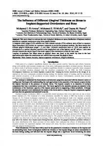
Figure 1. Geometric details and initial mesh configuration The Figure 1 shows the desired chip separation surface and desired machined surface separated by a narrow line of sacrificial layer of elements called damage zone, width of which has been mentioned as ε . It is noted that in reality these two surfaces should be same but such assumption has been taken only for the modeling purpose as a chip separation criterion where in ε → 0 . Consequently, a very small value of ε (0.04 mm) which is computationally acceptable has been taken as the width of the damage zone. The choice of the height of the designated damage zone is purely based on computational efficiency. It could be reduced further if faster computing facilities are available. The material model is defined for the entire workpiece while the damage model is defined specifically in the damage zone such that when the accumulated damage in an element in the sacrificial layer immediately ahead of the tool exceeds one, the element is supposed to fail. It is then removed from the mesh and consequently the tool moves further into the workpiece. Note that the fracture as such is not modeled. Table 1. Details of the geometric model and cutting parameters Description Cutting tool

Workpiece model geometry

Cutting parameters

Parameter Rake angle, γ

Value

−6o

Clearance angle, α

5o

Length (mm)

8

Width (mm)

0.4

Damage zone width (mm)

0.04

Feed, f (mm)

0.2

Cutting Velocity, Vc (m/min)

100

Element formulation Four-node plane strain bilinear quadrilateral (CPE4RT) elements with reduced integration scheme and hourglass control are used for the discretization for both the workpiece and the cutting tool. The workpiece is meshed with 2331 CPE4RT type elements by unstructured grid generation which utilizes advancing front algorithm in ABAQUS/Explicit. Since the elements produced by this method follow the boundary nodes, the resulting mesh may involve some skew in the element as observed in certain regions. Finite element formulation of this type of element is based on the isoparametric procedure i.e., the element geometry and the displacements are interpolated in the same way. The nodal degrees of freedom (DOF) of the quadrilateral element are shown in Figure 2.

Figure 2. Description of 2D quadrilateral element

The element geometry and displacement field are defined in terms of nodal coordinates and DOFs by the following functions: 4 ⎧ x = N i (ξ ,η ) xi ∑ ⎪ ⎪ i =1 ⎨ 4 ⎪ y = N (ξ ,η ) y ∑ i i ⎪⎩ i =1

4 ⎧ u = N i (ξ ,η ) ui ∑ ⎪ ⎪ i =1 ⎨ 4 ⎪v = N (ξ ,η ) v ∑ i i ⎪⎩ i =1

⇒ u =Nq

(1)

where xi , yi = global x-y coordinates at i-th node ui , v i = displacements at i-th node along global X, Y axes, respectively N i (ξ ,η ) = interpolation or shape function for i-th node defined in the natural coordinates

ξi ,ηi = natural coordinates of the i-th element node The nodal interpolation function N i (ξ ,η ) for quadrilateral elements is of the form (Liu & Quek, 2003): N i (ξ ,η ) =

1 (1 + ξiξ )(1 + ηiη ) for i = 1, 2,3, 4 4

(2)

The strains at any point within element can be expressed as follows: ⎡ ∂u ⎤ ⎡∂ ⎢ ⎥ ⎢ ⎡ε x ⎤ ⎢ ∂x ⎥ ⎢ ∂x ⎢ ⎥ ⎢ ∂v ⎥ ⎢ ⎢ε y ⎥ = ⎢ ⎥ = ⎢0 ⎢γ ⎥ ⎢ ∂y ⎥ ⎢ ⎣ xy ⎦ ⎢ ∂v ∂u ⎥ ⎢ ∂ ⎢ + ⎥ ⎢ ⎣ ∂y ∂x ⎦ ⎣ ∂y

0 ∂v ∂y ∂ ∂x

⎤ ⎡∂ ⎥ ⎢ ⎥ ⎢ ∂x ⎥ ⎡u ⎤ ⎢ ⎥ ⎢v ⎥ = ⎢0 ⎥⎣ ⎦ ⎢ ⎥ ⎢∂ ⎥ ⎢ ⎦ ⎣ ∂y

0 ∂v ∂y ∂ ∂x

⎤ ⎡u1 ⎤ ⎥ ⎢ ⎥ v1 ⎥⎥ ⎢ ⎥ ⎡ N1 0 N 2 0 N 3 0 ⎤ ⎥ ⎢0 N 0 N 0 N ⎥ ⎢ ⎥ ⎥ 1 2 4 ⎦⎢ ⎥⎣ u2 ⎥ ⎢ ⎥ ⎢v ⎥ ⎥ ⎣ 3⎦ ⎦

∴ ε = du = dNq = Bq

(3)

(4)

where B = strain-displacement matrix and q =vector of nodal displacements. Finally the stress- strain relationship becomes

σ = Dε = DBq

(5)

where D is the elasticity matrix defining the mechanical properties of the material in terms of the Young’s modulus and the Poisson’s ratio.

Boundary conditions For the simulation of cutting operation, proper type of boundary conditions should be imposed. The kinematic boundary conditions are as follows: For the workpiece:

u y = 0 on AB, u x = 0 on BC, vx = Vc on ABEF

(6)

where vx is the velocity in X-direction, Vc is the cutting velocity, and AB, BC and ABEF refer to edges in Figure1. For the cutting tool, boundary conditions on sides ON and MN in Figure1 are: u x = 0 on ON, u y = 0 on MN

(7)

The thermal boundary conditions are as follows: In case of adiabatic analysis, no heat transfer is allowed from the top surface of the workpiece, exposed surface of the chip and the machined surface to the cutting tool and to the atmosphere, i.e.,

∂T = 0 . While for the coupled temperature displacement analysis, boundaries CDF ∂n

and LM in Figure1 have convective heat transfer boundary conditions, with the overall heat transfer coefficient ( h ) , thermal conductivity ( k ) and ambient temperature (To ) given as input: −k

∂T = h (To − T ) ∂n

(8)

Rest of the surfaces for both tool and work piece were initially kept at (To ) . It is noted that the heat transfer coefficient h , being the ratio of average heat flow across the interface to the temperature drop, is a function of several variables such as, contact pressure, temperature, contacting materials, etc. Due to difficulties in measuring temperatures at tool-chip interface, there is hardly any data available for heat transfer coefficient for chip formation process. In the present work, simulations at a particular speed-feed combination were done for h varying within a range of 100-1000 kW/m 2 K. Since the difference in temperature was found to be very less with the change in heat transfer coefficient, h = 500 kW/m 2 K was considered as a fair compromise. Moreover, this value has also been used by Coelho (2006) for machining AISI 4340 and thus, taken as the reference value for the entire set of simulations.

Governing Equations The governing equations of a body undergoing deformation consists of two sets of equations, namely, the conservations laws of physics and the constitutive equations. The conservation laws can be applied to body of any material. But to distinguish between different materials undergoing deformation of varied degrees, one needs the constitutive equations.

Conservation laws Proper implementation of kinematics is important while developing a FE model for chip formation process. These kinematics refer to the mass, momentum and energy equations governing the continuum, which are given as follows:

ρ + ρ div v = 0

(9)

ρ v = f + div σ ρ e = σ : D − div q + r

(10) (11)

where ρ is the mass density, v material velocity, f body forces, σ Cauchy stress tensor, e specific internal energy, D strain rate tensor, q heat flux vector and r is body heat generation rate. The

superposed ‘ • ’ denotes material derivative in a Lagrangian description and ‘:’ denotes contraction of a pair of repeated indices which appear in the same order such as, A:B = Aij Bij . The basic idea of using FEM is to discretize the above equations and then to seek a solution to the momentum equation.

Work piece material constitutive equations Constitutive equations are a set of equations which describe the thermo-mechanical properties of a material undergoing deformation. Based on the simplicity or complexity of the material behaviour, there could be one constitutive equation or a set of constitutive equations that relate the deformation in the body to the stresses. It is assumed that elastic and inelastic responses are separable based on the fact that there is an additive relationship between the strain rates such that:

ε = ε e + ε pl

(12)

where ε is the total strain rate, ε e the rate of change of elastic strain and ε pl rate of change of plastic strain. This indicates initially the material responds elastically (recoverable) and when the stress is beyond the elastic limit, plastic deformation (non-recoverable) takes place. The elastic response can be described by simple linear elastic relationship given by:

σ = Del : ε el

(13)

where Del is the elasticity stress tensor and ε el is the elastic strain. The constitutive equations of plasticity usually contain yield criterion, flow rule and strain hardening rule. The yield criterion describes the stress state when yielding occurs, the flow rule defines increment of plastic strain when yielding occurs, and the hardening rule describes how the material is strain hardened as the plastic strain increases. For large deformation problems, as in case of machining, plasticity models based on von Mises yield criterion and Prandtl–Reuss flow rule are generally used to define the isotropic yielding and hardening (Wu, 2004). In case of machining process, isotropic yielding occurs when plastic deformation or straining occurs. The energy consumed here because of plastic deformation and tool-chip friction is converted largely into heat which raises the temperature in the cutting zone. Hence, realistic constitutive equations of plasticity (plasticity models) are an indispensable input in any FE simulations that are

efficient enough to describe stress-strain response as well as its dependence on strain rate, temperature and work hardening. The Johnson–Cook constitutive equation is one such model that is widely used to characterize the material behaviour of the workpiece satisfactorily (Johnson & Cook, 1983). This has been developed with data obtained from a series of Hopkinson bar tests at high strain rates and temperatures. The SHPB method enables to perform material tests at strain rates up to 104 s−1 by exposing the sample to stress waves. Furthermore, it can be used up to reasonable strains and can be tailored for tests at an elevated temperature (Jaspers & Dautzenberg, 2002). So far, this method has been found to be the most suitable one for the determination of mechanical behaviour of materials under conditions similar to those found in machining and thus, widely used in modeling of machining process (Shi and Liu, 2004; Umbrello et al., 2007; Davim & Maranhao, 2009; Vaziri et al., 2010). This model is also considered numerically robust as most of the variables are readily acceptable to the computer codes. The formulation of Johnson–Cook constitutive equation is based upon second deviatoric stress invariant flow theory with isotropic hardening which is defined as follows (Johnson & Cook, 1983; Johnson & Cook, 1985):

σ ′ = 2G(ε ′ − ε p ) εp =∫

2 p p ε : ε dt 3

(14) (15)

3 (16) σ ′ :σ ′ 2 where σ ′ is the deviatoric Cauchy stress, ε ′ is the deviatoric strain rate, ε p is the plastic strain rate,

σ=

ε p is the equivalent plastic strain, σ is the equivalent flow stress and G is the shear modulus. In this work, the following equivalent flow stress formulation has been used:

(

σ = A + B (ε ε∗ =

)

p n

)

m ⎛ ⎛ T −T ⎞ ⎞ room (1 + C lnε ) ⎜⎜1 − ⎜ T − T ⎟ ⎟⎟ ⎝ ⎝ m room ⎠ ⎠

εp for ε 0 p = 1 s-1 p ε0

p∗

(17) (18)

where Troom is the room temperature taken as 25 ºC, Tmelt is the melting temperature of the workpiece taken as 1520 ºC, A is the initial yield stress (MPa), B the hardening modulus, n the work-hardening exponent, C the strain rate dependency coefficient (MPa), and m the thermal softening coefficient.

These material parameters are fitted to the data obtained from a series of Hopkinson bar tests at high strain rates and temperatures. A ductile failure model is also incorporated, as a chip separation criterion, along with the material model in the damage zone in order to simulate the movement of the cutting tool into workpiece without any mesh distortion near the tool tip. Material failure refers to the complete loss of load carrying capacity which results from progressive degradation of material stiffness. Specification of damage model includes a material response (undamaged), damage initiation criterion, damage evolution and choice of element deletion. Damage initiation criterion is referred to as the material state at the onset of damage. In the present case, the damage model or failure model is based on Johnson-Cook damage initiation criterion. This model makes use of the damage parameter ωD defined as the sum of the ratio of the increments in the equivalent plastic strain Δε p to the fracture strain ε f (ABAQUS Theory manual), given as follows.

ωD = ∑

Δε p

(19)

εf

The fracture strain ε f is of the form as follows: ⎡

⎛ T − Troom ⎞ ⎤ ⎟⎥ ⎝ melt − Troom ⎠ ⎦

ε f = ⎣⎡ D1 + D2 exp ( D3σ ∗ ) ⎦⎤ × ⎣⎡1 + D4lnε p∗ ⎦⎤ × ⎢1 + D5 ⎜ T ⎣

σ∗ =

−P

σ

(20) (21)

where P is the hydrostatic pressure and D1 to D5 are failure parameters determined experimentally. The expression in the first set of brackets of Eq. (20) indicates the decrease in fracture strain as the hydrostatic pressure increases and the yield stress decreases. The damage initiation criterion is met when ωD reaches one. In machining, it is known that the maximum stress and strain occur in front of the cutting tool. With the advancement of tool the plastic strain increases within the workpiece material near the tool tip. Since damage model is defined, particularly, in the damage zone, as the plastic strain increases ωD of the elements in damage zone gradually reaches a value of one indicating that damage initiation criterion is met. Once the element satisfies the damage initiation criterion, Abaqus/Explicit assumes that progressive degradation of the material stiffness occurs, leading to

material failure based on the damage evolution. At any given time during the analysis, the stress tensor in the material is given by:

σ = (1 − D ) σ

(22)

where σ is the effective (undamaged) stress tensor computed in the current increment. When D reaches a value 1, it indicates that the material has lost its load carrying capacity completely. At this point, failure occurs and the concerned elements are removed from the computation. The ELEMENT DELETION = YES module along with the Johnson Cook damage model of the software enables to delete the elements that fail. This produces the chip separation and allows the cutting tool to penetrate further into the workpiece through a predefined path (damage zone). The Johnson–Cook material and damage constants for AISI 4340 standard alloy steel are given in Table 2 (Johnson & Cook, 1983; Johnson & Cook, 1985).

Table 2. Johnson-Cook parameters for AISI 4340 (Johnson & Cook, 1983; Johnson & Cook, 1985) A (MPa) B (MPa) 792

510

D1

n

C

m

0.26

0.014

1.03

0.05

D2

D3

D4

D5

3.44

−2.12

0.002

0.61

Thermo-mechanical properties of workpiece and cutting tool The physical properties of the AISI 4340 workpiece and the tungsten carbide cutting tool such as, density ( ρ ), Elastic modulus (E), Poisson’s ratio (ν ), specific heat ( C p ), thermal conductivity (k) and thermal expansion coefficient ( α ) are mentioned in Table 3 (Ozel & Zeren, 2006).

Table 3. Workpiece and cutting tool properties (Ozel & Zeren, 2006)

Material AISI 4340 Carbide tool

ρ 3

(kg/m )

E (GPa)

ν

Cp (J kg−1 K−1)

k (W m−1 K−1)

7850

205

0.30

475

44.5

11900

534

0.22

400

50

α (μm m−1K−1) 13.7 -

Interfacial contact and heat generation A kinematic contact algorithm has been used to enforce contact constraints in master-slave contact pair, where rake surface of the cutting tool is defined as the master surface and chip as the slave (node based) surface. This method conserves momentum between the contacting bodies. The kinematic contact algorithm works in two steps. Firstly, it determines which slave nodes in the predicted configuration penetrate in the surface and then calculates the resisting force required to oppose the penetration based on depth of each slave node’s penetration, mass associated with it and the time increment. Secondly, the contact algorithm determines the total internal mass of the contacting interfaces and calculates the acceleration correction for the master surface nodes. Acceleration correction for the slave nodes are then determined using the predicted penetration of each node, the time increment and the acceleration correction for the master surface nodes. This is required to obtain a corrected configuration in which the contact constraints are enforced. Both the frictional forces and the friction-generated heat are included in the kinematic contact algorithm through TANGENTIAL BEHAVIOUR and GAP HEAT GENERATION modules of the software. In actual practice, the stress distribution is not uniform over the rake face of the cutting tool, as shown in the Figure 3 (Zorev, 1963). It is assumed that no relative motion occurs between the tool and the chip when the normal stress is very large and the frictional stress is equal to the equivalent shear stress τ max . This region is called sticking zone ( Lstick ). On the contrary, in the sliding zone

( Lslip ), normal stress is small and frictional stress is proportional to the normal pressure, σ n , through a constant coefficient of friction, μ . Relative sliding of chip on the rake surface occurs and thus, Coulomb’s law holds good for this phenomenon (Ng, 2002). Mathematically, frictional stress τ is given by:

Figure 3. Stress distributions over the rake surface of the tool 0 < x ≤ Lstick (sticking zone) ⎧τ , when μσ n ( x ) ≥ τ max τ ( x ) = ⎨ max ⎩ μσ n ( x ), for μσ n ( x ) ≤ τ max Lstick < x ≤ Ln (slipping zone)

(21)

A and A is the yield stress (MPa). 3 During the machining process, heat is generated in the primary shear deformation zone due

where τ max =

to severe plastic deformation and in the secondary deformation zone due to both plastic deformation

and the friction in the tool-chip interface. The steady state two dimensional form of the energy equation governing the orthogonal machining process is given as: ⎛ ∂ 2T ∂ 2T ⎞ ⎛ ∂ 2T ∂ 2T ⎞ k ⎜ 2 + 2 ⎟ T − ρ Cp ⎜ u x 2 + v y 2 ⎟ + q = 0 ∂y ⎠ ∂y ⎠ ⎝ ∂x ⎝ ∂x q = qp + qf qp = η pσε

p

(24) (25) (26)

qf = ηf Jτγ (27) where q p is the heat generation rate due to plastic deformation, ηp the fraction of the inelastic heat, qf is the volumetric heat flux due to frictional work, γ the slip rate, ηf the frictional work conversion factor considered as 1.0, J the fraction of the thermal energy conducted into the chip, and

τ is defined in Eq. (21). The value of J may vary within a range, say, 0.35-1 for carbide cutting tool and AISI 4340 workpiece material (Mabrouki & Rigal, 2006). In the present work, 0.5 (default value in ABAQUS) has been taken. The fraction of the heat generated due to plastic deformation remaining in the chip, ηp , is taken to be 0.9 (Mabrouki et al., 2004). Thus, partition of heat that actually goes to the chip is taken care by the software during simulation by combining both the heat fractions i.e., J and ηp giving an average value within a range of 70-80% of the total heat.

Solution procedure An ALE approach is incorporated to conduct the FEM simulation. As mentioned earlier, ALE technique combines the features of pure Lagrangian and Eulerian analysis. The adaptive meshing technique in ABAQUS/Explicit implements ALE approach that allows flow boundary technique without altering elements and connectivity of the mesh. The idea is generally to apply features of Eulerian approach for modeling the area around the tool tip, while Lagrangian form can be applied to the free surface of the chip. This avoids severe element distortion and entanglement in the cutting zone without the use of remeshing criterion.

ALE formulation In the ALE approach, the grid points are not constrained to remain fixed in space (as in Eulerian description) or to move with the material points (as in Lagarangian description) and hence have their own motion governing equations. Hence, the Eqs. (9) to (11) can be rewritten according to the ALE description such that:

∼

•

( ) = ( )+ c ∇ ( )

(28)

c = v − vˆ

(29)

where superposed ‘ ∼ ’ is defined in the ALE description, c is the convective velocity, v is the material velocity, vˆ is the grid velocity and ∇ is the gradient operator. Consequently, the conservation laws are as follows:

ρ + c ∇ρ + ρ div v = 0 ρ v + ρ c ∇v = f + div σ ρ e + ρ c ∇e = σ : D − div q + r

(30) (31) (32)

FEM is basically used for discretizing the domain of interest into finite number of elements. The corresponding discretized equations of the above equations are obtained by employing the divergence theorem, the variational forms associated with these equations and finally using the Galerkin approach (Hutton, 2004). As a consequence, this leads to the metrical form of the conservative equations given as follows:

M ρ ρ + Lρ ρ + K ρ ρ = 0 M v v + Lv v + f int = f ext M e e + Le e = r

(33) (34) (35)

where M ρ , M v , M e are the generalized mass matrices for the corresponding variables, Lρ , Lv , Le are the generalized convective matrices, K ρ is the stiffness matrix for density, f int is the internal energy force vector, f ext is the external load vector and r is the generalized energy source vector. These matrices are defined in terms of shape functions of the elements and force vectors are defined in terms of shape functions, body force as well as traction acting on the surface (including contact forces).

Explicit dynamic analysis The explicit dynamic ALE formulation is primarily used to solve highly non-linear problems involving large deformations and changing contact, as observed in the case of machining. The explicit dynamic procedure in ABAQUS/Explicit is based upon the implementation of an explicit integration scheme for time dicretization of Eqs. (33) to (35). This analysis calculates the state of a system at a later time from the state of system at the current time. The explicit formulation advances the solution in time with the central difference method:

(

(i)

v i = M -1 f ext − f int

(i )

)

(36)

Δt ( i +1) − Δt i i (37) =v + v v 2 Δt ( i +1) − Δt i (i +1/ 2) (38) x ( i +1) = xi + v 2 where v is the velocity and v is the acceleration, M is the lumped mass matrix, f ext is the external ( i +1/ 2)

( i −1/ 2)

force vector and f int is the internal force. The subscript (i) refers to the increment number (i–1/2) and (i+1/2) and refer to mid-increment values. Since the kinematic state can be obtained using known values of and from the previous increment, the central difference integration operator is said to be explicit. The explicit procedure integrates through time by using many small time increments. The central difference operator is conditionally stable and the stability limit for the operator is based upon a critical time step. The critical time step for a mesh is considered to be the minimum taken over all the elements which is given by: Δtcrit ≤ min ( Le ce )

(39)

where Le is the characteristic length of the element and ce is the current wave speed of an element. When explicit dynamic ALE formulation is used, it introduces advective terms into the conservation equations to account for independent mesh motion as well as material motion. Advection refers to the process of mapping solution variables from an old mesh to a new mesh. In ALE approach, the solution for a time step advances step-wise. First part is a Lagrangian step which calculates the incremental motion of the material where the displacements are computed using the explicit integration rule and then all the internal variables are updated. Second part is referred to as an Eulerian or advection step where a mesh motion is performed to relocate the nodes such that the element distortion becomes minimum and the grid nodes can be moved according to any one or combination of the three algorithms namely, volumetric, Laplacian and equipotential smoothing. Then the element and the material variables are transferred from the old mesh to the new mesh in each advection step. In the present work, second order momentum advection (ABAQUS Theory manual) is carried out for the ALE mesh domains.

RESULTS AND DISCUSSION The type of chip formed affects the stress field generated in the workpiece which determines the residual stresses, cutting temperatures and cutting forces. Therefore, simulating the right kind of chip is essential for the proper analysis of the metal cutting process. This necessitates that FE simulations

have the capability to develop both continuous and segmented chips. The present work considers the machining of AISI 4340 with a negative rake carbide tool. Experimental studies available in the literature show that segmented chips are produced for such type of tool-workpiece combination, specifically at higher cutting speeds. Thus, the goal of this work is to develop a finite element model that not only simulates the saw-tooth chips but also explains the mechanism governing it. In this section, results dealing with von Mises equivalent stresses, equivalent strains, temperatures and machining forces during adiabatic analysis are presented showing the efficiency of this module to explain the chip formation phenomenon. But, in order to obtain more realistic results, fully coupled temperature displacement analysis was performed by considering the thermal conductivity of the workpiece in one case while neglecting it in the other case. Incorporating such variation in the given module shows the strong dependence of the chip morphology on thermal conductivity. Numerical results dealing with both the cases are presented and compared. The cutting force, thrust force and other related parameters were determined at different cutting speeds for each of the cases in coupled analysis. Feed values and cutting speeds are also varied for the chip formation in adiabatic analysis. Simulated results are then compared with each other as well as with the results available in the literature; thus, proving the validity of the developed FE model. The comparative study of the continuous and the segmented chips developed demonstrates the critical importance of modeling the correct type of chip.

Finite element modeling based on adiabatic analysis As already mentioned, there is very less time for the heat conduction to occur at higher cutting speeds during machining and thus adiabatic hypothesis can possibly be imposed for the modeling of the chip formation process.

Chip morphology and its mechanism Saw teeth or segmented chips are produced under adiabatic conditions with cutting parameters set at

Vc = 100 m/min and f = 0.2 mm . The chip segmentation is the result of a softening state at elevated temperatures during tool-workpiece interaction. Figures 4 (a–c), 5 (a–c) and 6 (a–b) are presented that help in explaining the mentioned phenomenon elaborately, by focusing on the formation of one chip segment only (onset at about 0.182 ms, segmentation at about 0.747 ms and final state at 0.9 ms).

Figure 4. von Mises equivalent stresses (Pa) at (a) 0.182 ms, (b) 0.747 ms and (c) 0.9 ms

Figure 5. von Mises equivalent strains at (a) 0.182 ms, (b) 0.747 ms and (c) 0.9 ms Figure 6. Temperature distribution (°C) at (a) 0.182 ms, (b) 0.747 ms and (c) 0.9 ms Figure 7 shows the cutting force ( Fc ) and thrust force ( Ft ) developed during the process.

Figure 7. Variation of the Fc and Ft at 0.182ms, 0.747 ms and 0.9 ms Chip formation begins with the bulging of the workpiece material in front of the tool as shown in the Figure 3(a). It can be seen that the stresses with the higher values are mainly distributed in the primary shear deformation zone, values ranging between 1.19–1.31 GPa, followed by the secondary shear deformation zone. At a particular instant, the stress along the primary shear zone becomes so high that it causes higher strains, ranging from 2–2.5 as shown in Figure 5 (a), and results in material damage. This causes a plastic deformation and localized heating. Consequently, rapid increase in temperature occurs near the tool tip that extends towards the chip free side causing the shear bands, known as the adiabatic shear bandings, to form. From the Figures 6 (b–c), it is noted that the temperature in the primary shear deformation zone becomes as high as 600–700°C which continues to increase as we move towards the chip free side. The maximum temperature is observed at a highly localized region at the chip free side with a value reaching up to 800–950°C. This induces thermal softening on the back of the chip and decreases the chip thickness. Such high temperatures in the valleys of the saw tooth profile were also reported by Ng and Aspinwall (Ng et al., 1999). Then the repeated occurrence of bulging and the shear banding results in waved irregularities on the chip back in the form of saw-teeth. Temperature rises gradually at the time of bulging of the chip but increases rapidly once the shear banding begins to form. Accordingly, regions of low and high temperatures occur alternately thus, giving a stripped pattern of temperature distribution as illustrated in Figure 8. As the cutting continues, because of the bulging of the chip the chip thickness gradually increases and so also the cutting forces. But the chip thickness decreases suddenly due to rapid increase of temperature and

subsequent thermal softening. As a consequence, cutting force reduces sharply at point B as shown in Figure 7 and then increases as the next bulge starts to build up.

Figure 8. Temperature distribution (°C) for segmented chip at 2 ms during adiabatic analysis The segmented chip produced in the present case closely matches with the experimental results of Belhadi et al. (2005) found under equivalent cutting conditions i.e., Vc = 100 m/min and

f = 0.2 mm . The interval between teeth on the simulated chip is 0.292 mm (see Figure 8) as compared to the value of 0.28 mm obtained by Belhadi et al. (2005). However, the predicted cutting forces are found to be underestimated when compared with the experimental values of Belhadi et al. (2005) and Lima et al. (2005), with the former the deviation being 30% and with later 10% .

Variation of feed and cutting speed In order to validate the developed model, feed (uncut chip thickness) is varied over a range of 0.1– 0.4 mm and its effect on the cutting and thrust forces are studied and compared with the existing results. Figure 9 (a) shows the effect of feed rate on the turning forces Fc and Ft when cutting AISI 4340 steel at Vc = 100 m/min. The cutting force and thrust force, as expected, increase almost linearly with increasing feed rate (Lima et al., 2005); thus confirming the results obtained by the present model. Similarly, cutting speed was varied over a range of 60–180 m/min during the formation of the segmented chip by using adiabatic analysis and its effect on the cutting force and thrust force is shown in the Figure 9 (b).

Figure 9. Effect of the (a) feed and (b) cutting speed on Fc and Ft in adiabatic analysis It is observed that cutting force and thrust force remained almost constant over the varying cutting speeds. Similar observations were reported by Mabrouki et al. (2008) while simulating the segmented chips, considering adiabatic hypothesis, for machining of aluminium alloy. This is, however, not the case for experimental results as found by Lima et al. (2005), where in decrease of about 22% in the cutting force and 30% in the thrust force has been observed as the cutting velocity increases from 60 to 180 m/min for machining AISI 4340 using a carbide tool.

Finite element modeling based on fully coupled temperature-displacement analysis Adiabatic conditions in metal cutting, no doubt, make the study of chip formation simpler but are not completely acceptable as far as real machining conditions are considered. Thus, coupled temperature displacement analysis is considered that not only provides a more practical approach for the simulation of chip formation but also determines the temperature field on the tool surface. This information is very useful in the study of tool wear progress. To demonstrate the ability of the model to simulate both continuous and segmented chips, thermal conductivity of the workpiece is considered in one case while neglected in the other case. The cutting speed was varied in both the cases and its effect on the cutting force was studied. This parametric study, in one way, helps in validating the developed models.

Chip morphology When the thermal conductivity of the workpiece material was considered in the coupled temperature displacement analysis, continuous chips were obtained in contrast to the previous section where segmented chips, as found experimentally (Belhadi et al., 2005), were produced under the same cutting conditions. Figure 10 (a) shows the deformed finite element mesh for the continuous chip formation. Since adiabatic conditions allow maximum amount of heat to be retained on the chip surface, adiabatic shearing was very prominent; thus reproducing saw-teeth due to thermal softening on the back of the chip. While, in the case of coupled temperature analysis with thermal conductivity of the workpiece defined, heat conduction occurred and the heat generated due to plastic deformation was not confined to the primary shear deformation zone only. This produced uniform and continuous chips which in the present case is not the desired type of chip. On one hand, adiabatic hypothesis plays a vital role in simulating the segmented chips while on the other hand, these are unacceptable in real machining. Therefore, to simulate the correct type of chip in a more realistic manner, the simplest way is to combine the relevant features of both the approaches, i.e. to incorporate the adiabatic boundary conditions in the coupled temperature displacement analysis. It is possible by neglecting the thermal conductivity of the workpiece that allows the localized heating due to plastic

deformation to extend from the tool tip towards the chip free side. This induces thermal softening and consequently, the saw tooth profile on the back of the chip. Figure 10 (b) shows the deformed finite element mesh for the segmented chip formation by neglecting the thermal conductivity of the workpiece.

Figure 10. Deformed FE mesh for (a) continuous chip formation and (b) segmented chip formation Figures 11 (a–c) and 11 (a–c) clearly depict the variation in distribution of equivalent von Mises stresses, equivalent strain and the temperature over the chip surface when the chip morphology changes.

Figure 11. (a) von Mises equivalent stresses, (b) von Mises equivalent strains and (c) Temperature distribution (°C) for continuous chip formation

Figure 12. (a) von Mises equivalent stresses (Pa), (b) von Mises equivalent strains and (c) Temperature distribution (°C) for segmented chip formation From Figures 11 (a) and 12 (a), it is observed that the levels of stresses for both the cases were similar but the distribution pattern of the stresses varied significantly for continuous and segmented chips. In the segmented chips highly localized stresses were found in the shear zone with values in the range of 1.19–1.24 GPa; same as those found in the case of adiabatic analysis. While in continuous chips the stresses are distributed over a wider region over the chip surface. Similar comparisons were reported by Ng and Aspinwall (1999) and Wu and Matsumoto (1990), thus confirming the results obtained. Figures 11 (c) and 12 (c) show that the distribution of temperature over the chip surface, again, differs considerably in both the cases. The shear zone temperature for continuous chip was found to be lower, in the range of 250–300°C as compared to the segmented chips. During the formation of segmented chips, shear zone temperature initially falls in this range but then gradually attains a higher value of 430–460°C. This increased temperature in the shear zone of segmented chips is attributed to highly localized stresses and strains as shown in Figures 12 (a–b), respectively. Highest temperatures were observed along the tool-chip interface for the continuous chips, specifically in the sliding zone of the rake surface, the value corresponding to 550–566°C. As one

moves from the tool tip towards the chip free surface, temperature decreases to 400°C. Shih (1996) found the location of maximum temperature in the same region while simulating the continuous chip formation. With segmented chips, higher temperatures are observed in the valleys of the saw tooth along with the tool chip interface region. The temperature at these valleys was found to be around 500°C. The temperature profile obtained in this case is similar with the one obtained in the previous section by adiabatic analysis (See Figure 8) with the difference that higher values of temperatures were obtained in the shear banding region for adiabatic analysis. Besides, the bending of the chip is also highly prominent in the latter case.

Cutting forces Figures 13 (a) and (b) show the evolution of the forces Fc and Ft over time and distribution of the normal stress σ n and frictional stress τ on the rake surface for both continuous and segmented chip formation, respectively.

Figure 13. (a) Evolution of Fc and Ft over time and (b) Distribution of σ n and τ on the rake surface for continuous and segmented chip formation The force signature shows that the cutting force corresponds to the type of chip produced in the cutting process. During continuous chip formation, the cutting force did not show much fluctuation. Whereas, in the case of segmented chip formation, cutting force fluctuates due to change in the deformed chip thickness and thus, shows prominent depletion and accumulation of stresses. It is also noted that the formation of continuous chips exhibited higher value of cutting force. Since the thermal conductivity of the workpiece material was negligible in the case of segmented chips, the material deformed more easily leading to lower value of cutting force. Baker (2003) also found that cutting force is the largest for the case of no segmentation and degree of segmentation decreases as the conductivity is increased. As already mentioned, bending of the chip was also highly prominent when the thermal conductivity of the workpiece was neglected. As a consequence, the tool chip contact length decreased. This is much clear in the Figure 13 (b) which shows the normal stress and frictional stress distribution on the rake surface for continuous as well as segmented chip formation.

It is observed that the normal stress reaches its maximum value at a short distance away from the tool tip because no load acts at this location as the element gets deleted. Then gradually the normal stress decreases to zero at the point where the chip leaves the rake surface; thus indicating the tool-chip contact length (Shi et al., 2002). Since tool chip contact length is smaller for segmented chips, cutting force is lower. Besides, cutting forces are also known to vary with the deformed chip thickness. Thus, this can be attributed to the higher value of cutting force in continuous chip formation because a larger deformed chip thickness was observed with continuous chips.

Variation of cutting speed The cutting speed was varied over a range of 60–180 m/min at a feed of 0.2 mm for both continuous and segmented chip formation. Figures 14 (a) and (b) show the variation of Fc and the Ft

at

different cutting velocities for continuous chips and segmented chips, respectively. It is known that as the cutting velocity increases the cutting force and thrust force decrease. The reason for this can be explained from the expressions of the cutting force and thrust forces which are given as follows: Cutting force, Fc = tsτ s (ζ − tan γ + 1) Thrust force, Ft = tsτ s (ζ − tan γ − 1) ,

(40) (41)

where, t is the depth of cut (mm), s is the feed rate (mm/rev), τ s is the dynamic shear strength of the workpiece, γ is the rake angle and ζ is the chip reduction coefficient, i.e. the ratio of deformed chip thickness to undeformed chip thickness.

Figure 14. Variation of Fc and Ft for (a) continuous chip and (b) segmented chip at different cutting velocities As the cutting velocity increases, temperature of the shear zone increases. This causes softening of the work piece, which means the value of τ s decreases and thereby reduces the value of cutting and thrust force as shown in Figures 15 (a) and (b). In Figure 14 (a), it is observed that cutting force reduced by 11% as the cutting velocity is varied from 60 m/min to 180 m/min. However, not much reduction is observed in the thrust forces. Figure 14(a) shows the corresponding increase of mean temperature in the primary shear deformation zone with cutting velocity, during continuous chip formation for a simulation time of 1 ms.

Figure 15. Temperature history of nodes in primary shear deformation zone at Vc = 60, 100 and 180m/min for (a) continuous chip and (b) segmented chip From Figure 14 (b), it is observed that the cutting force reduced by 10% as the cutting velocity increased from 60 m/min to 100 m/min but remained almost constant even when the cutting velocity was increased to 180 m/min. Such an unexpected behavior can be attributed to the adiabatic hypothesis considered by neglecting the thermal conductivity of the workpiece. When the thermal conductivity is neglected, it possibly does not take into account the softening of the workpiece material which actually occurs near the tool tip due to increased temperature at high cutting speeds; thus showing fairly constant value at higher cutting speeds. The variation of mean shear zone temperature at variable cutting speeds for a simulation time of 1ms, presented in Figure 15 (b), explains this phenomenon fairly well. Although the temperature in the primary shear deformation zone has increased when cutting speed increased from 100 m/min to 180 m/min, there is no change in the corresponding forces. One more reason for the decrease of these forces is that the value of chip reduction ratio ζ decreases by a small amount as the cutting velocity, shown in Figure 16 (a), increases. The reason for such variation can be explained from the expression of ζ which is given as follows (Bhattacharyya, 2006):

ζ = cot β cos γ + sin γ

(42)

As the cutting velocity increases, the shear zone shrinks and results in the increase of shear angle β which in turn decreases the chip reduction ratio, ζ . Consequently the deformed chip thickness decreases as shown in Figure 16 (b). The tool-chip contact length ( Ln ) which in turn affects the cutting force considerably, also changes with variable cutting speed. Figure 16 (c) shows effect of cutting velocity on tool-chip contact length for both continuous and segmented chip formation.

Figure 16. Variation of (a) chip reduction ratio (b) deformed chip thickness and (c) tool-chip contact length with cutting velocity for continuous and segmented chip formation

Chip reduction coefficient, deformed chip thickness and tool-chip contact length showed fairly constant value at higher cutting speeds during the formation of segmented chip formation as observed in the case of forces.

Verification of simulated results Verification of FE model is the final and mandatory stage of the FEM authentication in metal cutting. As far as the authenticity of the present model is concerned, predicted results are compared with the experimental results presented by Lima et al. (2005) for machining AISI 4340 using carbide cutting tool ( γ = −6 º) under similar cutting conditions. Figure 17 shows the deviation between experimental values (Lima et al., 2005) of cutting force and the thrust force with that of the predicted values, as deduced from the simulation of continuous and segmented chip formation. It is found that the simulated results lie well within the acceptable range. In case of continuous chip formation, the cutting force and thrust values closely match with that of the experimental ones, with largest deviation not more than 12-13% observed for low cutting speed (60 m/min). In case of segmented chip formation, both the forces show underestimated values over the considered cutting speed range with maximum deviation not exceeding 20%. It is interesting to note that predicted results, for both continuous and segmented chip formation, showed maximum deviation at the lowest cutting speed, while in higher cutting speeds the values are closer to the experimental ones.

Figure 17. Comparison of predicted forces during simulation of continuous and segmented chip formation with experimental forces

Discussion The present work shows that stress, strain and temperature fields are greatly affected by the chip formation process. Since the goal is to focus on the segmented chip formation, adiabatic analysis module of ABAQUS/Explicit was used at the beginning. Well-defined adiabatic shear bandings are observed in this case as no heat conduction is allowed during the machining process. When feed rate was varied, the cutting force and thrust force increased, as expected. On the other hand, when the cutting speed was varied, the forces remained almost constant. This emphasizes that ignoring the heat conduction completely is impractical, though it produces prominent saw tooth chips based on adiabatic shearing. Hence, coupled temperature displacement analysis was employed to make the

study more realistic. In this study, an attempt was made to simulate both continuous and segmented chip formation. Continuous chips were produced when thermal conductivity of the workpiece was defined in the coupled temperature displacement analysis as compared to the segmented chips produced in the experimental findings of Belhadi et al. (2005) under similar cutting conditions. During continuous chip formation, stress fields are not as localized in primary shear zone as observed in the case of segmented chip. As a consequence, highest equivalent strains and temperature levels are not found in this region, but in the secondary shear deformation zone. The chip which is entering into the secondary shear deformation zone already possesses accumulated plastic strain and heat. The instant it begins to flow over the rake surface, further plastic straining and local heating occurs because of severe contact and friction in the contact zone (Shi et al., 2002). Therefore, the maximum equivalent plastic strain and temperature are found along the tool-chip interface, specifically in the sliding region in contrast to segmented chip formation during adiabatic analysis where maximum temperature is shown at the back of the chip as no heat conduction exists between rake surface and the chip surface. Though the desired chip morphology could not be predicted with this module, the cutting forces were found to match closely with the experimental ones. This motivated to combine the adiabatic hypothesis, as considered in adiabatic analysis (predicting desired chip morphology) with the coupled temperature-displacement analysis (predicting forces satisfactorily). Hence, the thermal conductivity of the workpiece was simply neglected in the coupled analysis to cater to the present need of generating segmented chips. In this case, maximum values of temperature are observed in the secondary shear zone due to high straining along the tool-chip interface as well as at the back of the chip in a highly localized region that induces thermal softening causing the desired saw tooth profile. The present work focuses on predicting the right kind of chip morphology. It is known that type of chip produced depend upon the type of cutting tool and workpiece materials, cutting conditions and so on. Chip morphology is an important index in the study of machining because it affects the stress field generated in the workpiece which determines the residual stresses, the cutting temperatures and the cutting force. Determination of the cutting forces facilitate estimation of power consumption which is required for the design of machine-fixture-tool system, evaluation of role of various machining conditions and condition monitoring of the cutting tools. The variation in the cutting force has been

shown to be related to the chip morphology. A smoother time signature of the cutting force indicates continuous chip formation with good surface finish whereas wavy time signature of the cutting force indicates segmented chip formation. Obviously, magnitude of the waviness (difference between the peak and lower values) relates to surface finish quality. It is also important to consider the regularity of the waviness which indicates the intervals (time interval correlates to space interval at known cutting conditions) at which residual stresses are released. The developed model beautifully exposes these physical understandings. Moreover, the knowledge of the cutting temperature gives idea about the tool wear progress, residual stresses and the surface finish of the machined surface. It is, thus, clear that controlling these variables can lead to higher productivity and accuracy which in case of metal cutting leads to higher tool life and better surface finish. The stresses, strains, temperatures and many other outputs that are obtained from FE simulations greatly help in understanding the basic mechanism of chip formation under different cutting conditions. Note that various aspects of metal cutting like, cutting tool design, optimization of cutting parameters for higher tool life and good surface finish, prediction of tool wear growth, etc. are achievable only when we are able to comprehend the underlying physics of the chip formation process correctly by simulating right kind of chip morphology under different cutting conditions.

CONCLUSIONS A 2D plane strain FE model has been developed by using simulation software ABAQUS/Explicit with appropriate material and damage models. Numerical results showed that adiabatic hypothesis plays a crucial role in the formation of segmented chips due to adiabatic shearing. Adiabatic analysis module proved useful in explaining formation of adiabatic shear banding that consequently lead to thermal softening and thus the formation of saw-tooth chips during machining of AISI 4340 steel. However, this module was unable to satisfactorily show the effect of the cutting speed on the turning forces. In coupled temperature displacement analysis, simulation of continuous and segmented chip formation was demonstrated successfully. Thermal conductivity of the workpiece was neglected to satisfy the adiabatic hypothesis for simulating the formation of segmented chip. Highest temperature levels were observed only along the tool-chip interface during continuous chip formation. But during

the formation of segmented chip formation, temperatures closer to tool-chip interface temperature were found in highly localized regions at the back of the chip. Such variations in temperatures are attributed to the corresponding variation in the stress and strain fields. Prediction of right kind of chip morphology is important as it affects the stress field generated in the workpiece which determines the residual stresses, the cutting temperatures and the cutting force. It has been shown that there exists a correlation between the type of chip produced and the time signature of the cutting force. Knowledge of the cutting forces are useful in estimation of power consumption which is required for the design of machine-fixture-tool system, evaluation of role of various machining conditions and condition monitoring of the cutting tools. It is found that the predicted forces for segmented chips by neglecting the thermal conductivity are underestimated when compared with the experimental values (Lima et al., 2005) and the simulated values for continuous chip formation. This approach can still be considered as a fair compromise because it not only simulates the desired segmented chips and but also, predicts the cutting force and thrust values with maximum deviation not exceeding 20%. Moreover, the difference between the predicted and the experimental values are prominent in low cutting speed. It is observed that as the cutting speed increases the deviation in the predicted values gradually decrease. This can be attributed to the fact that at higher cutting speeds adiabatic hypothesis satisfies well whereas at lower cutting speeds the assumption shows inadequacy.

REFERENCES Akarca, S. S., Song, X., Altenhof, W. J. & Alpas, A. T. (2008). Deformation behaviour of aluminium during machining: Modelling by Eulerian and smoothed-particle hydrodynamics methods. Proceedings of the Institute of Mechanical Engineers –J of Materials: Design and Applications, 222, 209-219 Attanasio, A., Cerretti, E., Rizzuti, S., Umbrello, D. & Micari, F. (2008). 3D finite element analysis of tool wear in machining. CIRP Annals - Manufacturing Technology, 57(1), 61-64 Baker, M. (2005). Does chip formation minimize energy, Computational Materials Science, 33, 407-418 Baker M., Rosler J. & Seimers, C. (2002). A finite element model of high speed metal cutting with adiabatic shearing. Computer and structures, 80, 495-513 Baker, M., Rosler, J. & Seimers, C. (2002). Finite element simulation of segmented chip formation of Ti6Al4V. Journal of Manufacturing Science and Engineering, 124, 485-488 Baker, M. (2003). An investigation of the chip segmentation process using finite elements. Technische Mechanik, 23, 1-9

Bhattacharyya, A. (2006). Metal cutting theory and practice. Central Book Publishers Calamaz, M., Coupard, D. & Girot, F. (2008). A new material model for 2D numerical simulation of serrated chip formation when machining titanium alloy. International Journal of Machine Tools and Manufacture, 48, 275-288 Coelho, R. T., Ng, E. -G. & Elbestawi, M. A. (2006). Tool wear when turning AISI 4340 with coated PCBN tools using finishing cutting conditions. Journal of Machine tools & Manufacture, 47 (1-2), 263-272 Davim, J. P. & Maranhao, C. (2009). A study of plastic strain and plastic strain rate in machining of steel AISI 1045 using FEM analysis. Materials and Design, 30, 160–165 Elbastwani, M. A., Srivatava, A.K. & Wardany, E. l-. (1996). A model for chip formation during machining of hardened steel. Annals of CIRP, 45, 71-76 HKS ABAQUS Theory manual (version 6.7), Hibbit, Karlsson and Sorens Inc., Pawtucket, USA. Hutton, D. V. (2004). Fundamentals of finite element analysis. Mc Graw Hill Iwata, K., Osakada, K. & Terasaka, Y. (1984). Process modeling of orthogonal cutting by the rigid-plastic finite element method. ASME Journal of Engineering Materials and Technology, 106, 132-138 Johnson, G. R. & Cook, W. H. (1983). A constitutive model and data for metals subjected to large strains, high strain rates and high temperatures. Proceedings of 7th International Symposium on Ballistics, the Hague, The Netherlands, 541–547 Johnson, G. R. & Cook, W. H. (1985). Fracture characteristics of three metals subjected to various strains, strains rates, temperatures and pressures. Engineering Fracture Mechanics, 21(1), 31-48 Jaspers, S. P. F. C & Dautzenberg, J. H. (2002). Material behavior in conditions similar to metal cutting: flow stress in the primary shear zone. Journal of Materials Processing Technology, 122, 322-330 Klamecki, B. E. (1973). Incipient chip formation in metal cutting- A three dimensional finite element analysis. Ph.D. thesis, University of Illinois, Urbana Komvopoulous, K. & Erpenbeck, S. A. (1991). Finite element modeling of orthogonal metal cutting. ASME Journal of Engineering for Industry,113, 253-267 Konig, W., Jinge, M. K. & Link, R. (1990). Machining with hardened steels with geometrically defined cutting edges. Annals of CIRP, 39, 61-64 Li, K., Gao, X. -L. & Sutherland, J. W. (2002). Finite element simulation of the orthogonal metal cutting process for qualitative understanding of the effects of crater wear on the chip formation. Journal of Materials Processing Technology, 127, 309-324 Lorentzon, J. & Jarvstrat, N. (2009). Modelling chip formation of alloy 718. Journal of Materials Processing Technology, 209, 4645-4653 Liu, G. R. & Quek, S. S. (2003). The finite element method: A practical course (Butterworth Heinemann,). Lima, J. G., Avila, R. F., Abrao, A. M., Faustino, M. & Davim, J. P. (2005). Hard turning: AISI 4340 high strength alloy steel and AISI D2 cold work tool steel. Journal of Materials Processing Technology, 169, 388-395 Mackerle, J. (1962). Finite element methods and material processing technology, an addendum (1994–1996). Engineering Computations, 15, 616-690

Mabrouki, T. & Rigal, J. -F. (2006). A contribution to a qualitative understanding of thermo-mechanical effects during chip formation in hard turning. Journal of Material Processing Technology, 176, 214-221 Movahhedy, M., Gadala, M. S. & Atlantis, Y. (2000). Simulation of the orthogonal metal cutting process using an Arbitrary Lagrangian Eulerian finite element method. Journal of Materials Processing Technology, 103, 267-275 Mabrouki, T., Deshayes, L., Ivester, R., Regal, J. -F. & Jurrens, K. (2004). Material modeling and experimental study of serrated chip morphology. Proceedings of 7th CIRP International Workshop on Model. Machin, France April 4-5 Mabrouki, T., Girardin, F., Asad, M. & Regal, J. -F. (2008). Numerical and experimental study of dry cutting for an aeronautic aluminium alloy. International Journal of Machine Tools and Manufacture, 48, 1187-1197 Ng, E. G., Tahany, I., Wardany, E-., Dumitrescu, M. & Elbestawi, M. A. (2002). Physics based simulation of high speed machining. Machining Science and Technology, 6, 301-329 Ng, E. G., Aspinwall, D. K. & Monaghan, D. (1999). Modeling of temperature and forces when orthogonally machining hardened steel. International Journal of Machine Tools and Manufacture, 39, 885-903 Ozel, T. & Zeren, E. (2006). A methodology to determine work material flow stress and tool-chip interfacial friction properties by using anaysis of machining. Journal of Manufacturing Science and Engineering, Transactions of the ASME, 128, 119-129 Ozel, T. (2006). The influence of friction models on finite element simulations of machining. International Journal of Machine Tools and Manufacture, 46, 518-530 Ohbuchi, Y. & Obikawa T. (2005). Adiabatic shear in chip formation with negative rake angle. International Journal of Mechanical Sciences, 47, 1377-1392 Olovsson, L., Nilsson, L. & Simonsson, K. (1999). An ALE formulation for the solution of two-dimensional metal cutting problems. Computers and Structures, 72, 497-507 Obikawa, T., Sasahara, H., Shirakashi, T. & Usui, E. (1997). Application of computational machining method to discontinuous chip formation. Journal of Manufacturing Science and Engineering, 119, 667-674 Raczy, A., Elmadagli, M., Altenhof, W. J. & Alpas, A. T. (2004). An Eulerian finite-element model for determination of deformation state of a copper subjected to orthogonal cutting. Metallurgical and Materials Transactions, 35A, 2393-2400 Rakotomalala, R., Joyot, P. & Touratier, M. (1993). Arbitrary Lagrangian-Eulerian thermomechanical finite element model of material cutting. Communications in Numerical Methods in Engineering, 9, 975-987 Strenkowski, J. S. & Moon, K. -J. (1990). Finite element prediction of chip geometry and tool/workpiece temperature distributions in orthogonal metal cutting. ASME Journal of Engineering for Industry, 112, 313-318. Strenkowski, J. S. & Carroll III, J. T. (1985). A finite element model of orthogonal metal cutting. ASME Journal of Engineering for Industry, 107, 349-354 Shi, J. & Liu, C. R. (2004). The influence of material models on finite element simulation of machining. Journal of Manufacturing Science and Engineering, Transactions of the ASME, 126, 849-857 Shih, A. J. (1996). Finite element analysis of orthogonal metal cutting mechanics. Journal of Machine Tools & Manufacture, 36, 255-273 Shi, G., Deng, X. & Shet, C. (2002). A finite element study of the effect of friction in orthogonal metal cutting. Finite Elements in Analysis and Design, 38, 863-883

Tay, A. O., Stevenson, M. G. & de Vahl Davis, G. (1974). Using the finite element method to determine temperature distribution in orthogonal machining, Proceedings of the Institute of Mechanical Engineers, 188(55), 627-638. Umbrello, D. M’Saoubi R. & Outeiro J. C. (2007). The influence of Johnson–Cook material constants on finite element simulation of machining of AISI 316L steel. International Journal of Machine Tools & Manufacture, 47, 462–470 Vyas, A. & Shaw, M. C. (1999). Mechanics of saw tooth chip formation in metal cutting. Journal of Manufacturing Science and Engineering, 121, 163-173 Vaziri, M.R. Salimi, M. & Mashayekhi M. (2010). A new calibration method for ductile fracture models as chip separation criteria in machining. Simulation Modelling Practice and Theory, 18, 1286–1296 Wu, D. W. & Matsumoto, Y. (1990). The effect of hardness on residual stresses in orthogonal machining of AISI 4340 steel. Journal of Engineering for Industry, 112, 245-252 Wu, H. -C. (2004). Continuum Mechanics and Plasticity. Chapman and Hall/CRC Zorev, N. N. (1963). Inter-relationship between shear processesoccuring along tool face and shear plane in metal cutting. International Research in Production Engineering, ASME, 42-49

Figures Figure 1. Geometric details and initial mesh configuration N

M

Desired chip separation surface

ε Tool Desired machined surface

C

D O

E B

L

Y Z

X

A

Figure 2. Description of 2D quadrilateral element

y, v 4 (x4, y4) (u4, v4)

η ξ

2b

3 (x3, y3) (u3, v3)

2a 2 (x2, y2) (u2, v2)

1 (x1, y1) (u1, v1)

x, u

Figure 3. Stress distributions over the rake surface of the tool

σ n ( x)

Workpiece

τ = τ max τ = μσ n ( x )

Lslip

Lstick

Ln

Figure 4. von Mises equivalent stresses (Pa) at (a) 0.182 ms, (b) 0.747 ms and (c) 0.9 ms

S, Mises (Avg: 75%) +1.433e+09 +1.314e+09 +1.194e+09 +1.075e+09 +9.553e+08 +8.359e+08 +7.165e+08 +5.971e+08 +4.777e+08 +3.582e+08 +2.388e+08 +1.194e+08 +0.000e+00

Y Z

X


Step: Step−1 Increment 135661: Step Time = 1.8250E−04 Primary Var: S, Mises Deformed Var: U Deformation Scale Factor: +1.000e+00 Status Var: STATUS


Y Z


X

(a)

Y Z

X


(b)

(c)

Figure 5. von Mises equivalent strains at (a) 0.182 ms, (b) 0.747 ms and (c) 0.9 ms

PEEQ (Avg: 75%) 3.71 3.40 3.09 2.78 2.47 2.16 1.85 1.54 1.24 0.93 0.62 0.31 0.00

PEEQ (Avg: 75%) 4.76 4.36 3.97 3.57 3.17 2.78 2.38 1.98 1.59 1.19 0.79 0.40 0.00

Y Z

X

Step: Step−1 Increment 135661: Step Time = 1.8250E−04 Primary Var: PEEQ Deformed Var: U Deformation Scale Factor: +1.00e+00 Status Var: STATUS

PEEQ (Avg: 75%) 4.26 3.91 3.55 3.20 2.84 2.49 2.13 1.78 1.42 1.07 0.71 0.36 0.00

Y Z

X


(a)

Y Z

X


(b)

(c)

Figure 6. Temperature distribution (°C) at (a) 0.182 ms, (b) 0.747 ms and (c) 0.9 ms

TEMP (Avg: 75%) 939.11 862.93 786.76 710.58 634.41 558.23 482.05 405.88 329.70 253.53 177.35 101.18 25.00

TEMP (Avg: 75%) 965.40 887.03 808.66 730.30 651.93 573.57 495.20 416.83 338.47 260.10 181.73 103.37 25.00

Y Z

X

Step: Step−1 Increment 135661: Step Time = 1.8250E−04 Primary Var: TEMP Deformed Var: U Deformation Scale Factor: +1.00e+00 Status Var: STATUS

(a)

TEMP (Avg: 75%) 939.11 862.93 786.76 710.58 634.41 558.23 482.05 405.88 329.70 253.53 177.35 101.18 25.00

Y

Y Z

X


(b)

Z

X


(c)

Figure 7. Variation of the Fc and Ft at 0.182ms, 0.747 ms and 0.9 ms 500

Force (N)

400

C

A Fc

B

300 200 100

Ft

0O 0.0 0.1 0.2 0.3 0.4 0.5 0.6 0.7 0.8 0.9 0.747ms 0.182ms Time (ms)

Figure 8. Temperature distribution (°C) for segmented chip at 2 ms during adiabatic analysis

TEMP (Avg: 75%) 939.11 862.93 786.76 710.58 634.41 558.23 482.05 405.88 329.70 253.53 177.35 101.18 25.00

Y

Z

X

Figure 9. Effect of the (a) feed and (b) cutting speed on Fc and Ft in adiabatic analysis

700

500

Fc Ft

600

400

Force (N)

Force (N)

500 400 300 200

300 200 100

Fc Ft

100 0

0.10

0.15

0.20

0.25

0.30

0.35

0 40

80

120

160

200

Cutting velocity (m/min)

Feed (mm)

(a)

(b)

Figure 10. Deformed FE mesh for (a) continuous chip formation and (b) segmented chip formation

Y

Y Z

Z

X

X

(a)

(b)

Figure 11. (a) von Mises equivalent stresses, (b) von Mises equivalent strains and (c) Temperature distribution (°C) for continuous chip formation


Y

Z

NT11 563.6 518.7 473.8 428.9 384.1 339.2 294.3 249.4 204.5 159.6 114.8 69.9 25.0

PEEQ (Avg: 75%) 4.96 4.55 4.13 3.72 3.31 2.89 2.48 2.07 1.65 1.24 0.83 0.41 0.00

Y

Y Step: Step−1 Increment 4059380: Step Time = 1.4000E−03 Primary Var: S, Mises Deformed Var: U Deformation Scale Factor: +1.000e+00 Status Var: STATUS

X

Z


X

(a)

Z

X

Step: Step−1 Increment 4059380: Step Time = 1.4000E−03 Primary Var: NT11 Deformed Var: U Deformation Scale Factor: +1.0e+00 Status Var: STATUS

(b)

(c)

Figure 12. (a) von Mises equivalent stresses (Pa), (b) von Mises equivalent strains and (c) Temperature distribution (°C) for segmented chip formation


PEEQ (Avg: 75%) 3.90 3.58 3.25 2.93 2.60 2.28 1.95 1.63 1.30 0.98 0.65 0.33 0.00

Y

Z

NT11 712.20 654.94 597.67 540.40 483.13 425.87 368.60 311.33 254.07 196.80 139.53 82.27 25.00

Y

X


(a)

Z

Y

X


(b)

Z

X

Step: Step−1 Increment 2321100: Step Time = 1.4000E−03 Primary Var: NT11 Deformed Var: U Deformation Scale Factor: +1.00e+00 Status Var: STATUS

(c)

Figure 13. (a) Evolution of Fc and Ft over time and (b) Distribution of σ n and τ on the rake surface for continuous and segmented chip formation 1.8

500 Fc(continuous) Ft(continuous) Fc(segmented) Ft(segmented)

300 200

Stress (GPa)

1.4

400 Force (N)

σn(continuous) τ (continuous) σn(segmented) τ (segmented)

1.6 1.2 1.0 0.8 0.6 0.4

100

0.2

0 0.0 0.2 0.4 0.6 0.8 1.0 1.2 1.4

0.0 0.0

Time (ms) (a)

0.1

0.2

0.3

0.4

0.5

0.6

Distance from the cutting edge (mm) (b)

Figure 14. Variation of Fc and Ft for (a) continuous chip and (b) segmented chip at different cutting velocities 500

500

300 200

Fc Vc=60/min Vc=100/min Vc=180/min

Ft Vc=60/min Vc=100/min Vc=180/min

400 Force (N)

Force (N)

400

300 200

Fc Vc=60m/min Vc=100m/min Vc=180m/min

Ft Vc=60m/min Vc=100m/min Vc=180m/min

100

100 0 0.0 0.2 0.4 0.6 0.8 1.0 1.2 1.4 Time (ms) (a)

0 0.0 0.2 0.4 0.6 0.8 1.0 1.2 1.4 Time (ms) (b)

Vc=60m/min Vc=100m/min Vc=180m/min

0.2

0.4

o

450 400 350 300 250 200 150 100 50 0.0

Temperature ( C)

o

Temperature ( C)

Figure 15. Temperature history of nodes in primary shear deformation zone at Vc = 60, 100 and 180m/min for (a) continuous chip and (b) segmented chip

0.6

0.8

1.0

500 450 400 350 300 250 200 150 100 50 0.0

Vc=60m/min Vc=100m/min Vc=180m/min

0.2

0.4

0.6

0.8

1.0

Time (ms) (b)

Time (ms) (a)

0.6

2.5

0.5

2.0 1.5 1.0 0.5 0.0

continuous chip segmented chip 60 80 100 120 140 160 180 Cutting velocity (m/min)

(a)

0.60

0.4 0.3 0.2 0.1 0.0

continuous chip segmented chip

Tool-chip contact length (mm)

3.0

Deformed chip thickness (mm)

Chip reduction ratio

Figure 16. Variation of (a) chip reduction ratio (b) deformed chip thickness and (c) tool-chip contact length with cutting velocity for continuous and segmented chip formation

0.45 0.30 0.15 0.00

continuous chip segmented chip

60 80 100 120 140 160 180

60 80 100 120 140 160 180



(b)

(c)

Figure 17. Comparison of predicted forces during simulation of continuous and segmented chip formation with experimental forces

600

Fc

500

Force (N)

400 Experimental (Lima et al., 2005) Simulation (continuous chip) Simulation (segmented chip)

300

200

Ft

100

0 60

80

100

120

140


160

180

A Finite Element Study of Chip Formation Process

A Finite Element Study of Chip Formation Process

Suggest Documents

A Finite Element Study of Chip Formation Process

Finite Element Simulation of Chip Formation during ...

A Finite Element Study

A Finite Element Analysis Study

Finite Element Study on Pre-Tightening Process of Threaded

A Finite Element Study On - IOSR Journals

Finite Element Simulation of a Friction Drilling process using Deform ...

Finite Element modeling of hard turning process via a

Finite Element Simulation and Validation of Chip ... - ScienceDirect

a finite element analysis

A Finite Element Analysis

A spectral finite element

a finite element analysis

A finite element analysis

A finite-element study of a piezoelectric/poroelastic sound ... - CiteSeerX

A large scale finite element study of a cementless ...

A Finite Element Model to Simulate Defect Formation during ... - MDPI

Finite-Element Parametric Study of the Consolidation Behavior of a ...

Finite-Element Parametric Study of the Consolidation Behavior of a ...

Tube Drawing Process Modelling By A Finite Element ...

A finite-element study of sapphire anvils for increased ...

A Unified Finite Element Approach for the Study of ...

Finite Element Design Study of a Rotating Disk Under ...

A Comparative Study of Galerkin Finite Element and B ...