A Framework for the Physical Design Problem for Data ... - CiteSeerX

A Framework for the Physical Design Problem for Data Synopses Arnd Christian K¨onig and Gerhard Weikum Department of Computer Science,University of the Saarland, P.O. Box 151150, 66041 Saarbr¨ ucken,Germany {koenig,weikum}@cs.uni-sb.de Abstract. Maintaining statistics on multidimensional data distributions is crucial for predicting the run-time and result size of queries and data analysis tasks with acceptable accuracy. Applications of such predictions include traditional query optimization, priority management and resource scheduling for data mining tasks, as well as querying heterogeneous Web data sources with diverse information quality. To this end a plethora of techniques have been proposed for maintaining a compact data ”synopsis” on a single table, ranging from variants of histograms to methods based on wavelets and other transforms. However, the fundamental question of how to reconcile the synopses for large information sources with many tables has been largely unexplored. This paper develops a general framework for reconciling the synopses on many tables, which may come from different information sources. It shows how to compute the optimal combination of synopses for a given workload and a limited amount of available memory. As the exact solution has large computational complexity, efficient heuristics are presented for limiting the search space of synopses combinations. The practicality of the approach and the accuracy of the proposed heuristics are demonstrated by experiments.

1

Introduction

Maintaining compact and accurate statistics on data distributions is of crucial importance for a number of tasks: (1) traditional query optimization that aims to find a good execution plan for a given query [5, 21], (2) approximate query answering and initial data exploration [13, 1, 18, 4, 12], (3) prediction of run-times and result sizes of complex data extraction and data analysis tasks on data mining platforms, where absolute predictions with decent accuracy are mandatory for prioritization and scheduling of long-running tasks (sometimes including the decision whether a given data analysis task can be expected to provide insight or should not be spawned at all). , and (4) estimation of the “information quality” of Web information sources (e.g., number of reviews per book in an e-commerce site) as a basis for planning global queries in a Web mediator [27] [28]. This broad importance of statistics management has led to a plethora of approximation techniques, for which [15] have coined the general term “data synopses”: advanced forms of histograms [30, 16, 20], spline synopses [22, 23], sampling [6, 17, 14], and parametric curve-fitting techniques [34, 9] all the way to highly sophisticated methods based on kernel estimators [2] or Wavelets and other transforms [26, 25, 4]. However, most of these techniques take the local

viewpoint of optimizing the approximation error for a single data distribution such as one database table with pre-selected relevant attributes. The equally important problem which combination of synopses to maintain on the application’s various datasets and how to divide the available memory between them has received only little attention [1, 8, 23], putting the burden of selecting and tuning appropriate synopses on the database administrator. This creates a physical design problem for data synopses, which can be very difficult in advanced settings such as predicting run-times of data analysis tasks or information wealth of Web sources by a mediator. The state of the art is inadequate for a number of reasons: – Since the accuracy of all approximation techniques depends on the memory size allotted to them, synopses for different data distributions compete for the available memory. In query optimization, for example, a small sized synopsis that does not improve query plan selection might have impact when given more memory. – All proposed techniques are limited in the types of queries they support well. Most techniques aim at range-query selectivity estimation only and are thus unsuitable for complex queries with joins or aggregation/grouping unless additional synopses are maintained that are geared for approximations that cannot be inferred from the base representations (e.g., join synopses [1, 23]). These additional synopses compete for the same memory space, and tuning the memory allocation for the various synopses is very difficult. – Because the choice of an optimal combination of synopses is dependent on the workload (i.e., the query mix for which run-time and result size predictions or approximate answers need to be computed), it needs to be continuously adapted to the evolving workload properties. The physical design problem for data synopses resembles the index selection problem for physical database design, which has been intensively studied [11, 10, 32] However, there are a couple of fundamental differences between these two problems that make the synopses problem much more difficult: (1) a synopsis not only chooses an attribute combination on which it maintains statistics, but its quality is highly dependent on the memory allocated to it (e.g., for a certain number of buckets in a histogram), and (2) a synopsis on a proper subset of attributes over which another synopsis is already maintained can be advantageous because of different approximation accuracies for different query types, whereas with B-tree indexes an index on a subset of an already indexed attribute combination would (to a first approximation) be superfluous. 1.1

Related Work

The reconciliation of different synopses as well as dedicated synopses for join queries (a uniform random sample over a foreign key join) was initially considered in [1]. Our work adapts these ideas and generalizes them, as their realization in the previous paper is limited to samples as base synopses and a data warehouse environment with a central fact table connected (via foreign keys) with

the respective dimension tables. An extension of this approach to incorporate workload information (in the form of access locality) can be found in [12], but it is also limited to the above scenario. The reconciliation problem for spline synopses was first discussed in [23], where a dynamic programming approach is proposed to minimize the error for a given set of synopses. However, this work offers no solution regarding which set of synopses to construct and does not take into account the characteristics of the workload. A similar approach for histograms was proposed in [19], extending [23] by offering heuristics that reduce the overhead of the dynamic programming problem. [8] considers a limited version of the problem: a set of synopses for query optimization are selected, based on whether or not they make a difference in plan selection. However, the approach is limited in a number of ways. Most importantly, synopsis selection is a series of yes-or-no decisions, with no consideration of the effect that variations of the size of a synopsis may have. This also has the consequence that the overall memory allotted to the selected synopses is utilized in a sub-optimal way. Furthermore, there is no consideration of special, dedicated (join-) synopses which do not constitute a (sub-)set of the attributes of a single relation. Otherwise, the approach to select synopses based on their effect on plan selection is orthogonal to the techniques of this paper and both can be combined, for example using the approach of [8] as part of the candidate selection in Section3.4. 1.2

Contribution and Outline

This paper develops a novel framework for the physical design problem for data synopses. Our framework covers the entire class of SPJ (i.e., select-project-join) queries. Note that projections are important also for predicting result sizes and run-times of grouping/aggregation, but have been almost completely ignored in prior work on data synopses. In contrast to the work in [8], our approach goes beyond the binary decisions on building vs. not building a certain synopsis, but also addresses the fundamentally important issue of how much memory each synopsis should be given. This is especially important when the role of statistics management goes beyond choosing good query execution plans, and synopses also serve to predict absolute run-times and result sizes, which in turn is highly relevant in data mining or Web source mediation environments. We characterize the exact solution for the optimal choice of synopses for a given workload. Taking into account the workload is a major step beyond our own prior work [23]. For complexity reasons, we derive various problem-specific heuristics that make our approach reasonably efficient and thus practical. The remainder of this paper is organized as follows. In Section 2 we define the underlying optimization problem, briefly review the relevant parts from earlier work on spline synopses [23], and introduce our error model. Section 3 then describes how to determine the optimal set of synopses exactly, using two assumptions which (in earlier experiments) have been found to hold for nearly all datasets and which lead to a compact formulation of the necessary computations. In Section 4 we show how to combine the various building blocks of our

framework into a unified algorithm. Section 5 contains an empirical validation of our approach in form of several experiments conducted with the TPC-H decision support benchmark. Finally, in Section 6 we summarize our work and give an outlook on future research.

2

Framework

We address the following optimization problem: given a number of datasets R := {R1 , . . . , Rn } and a workload consisting of SPJ (select-project-join) queries Q := {Q1 , . . . , Qk }, what is the best combination S of synopses such that the estimation error over all queries is minimized. We assume that each query Qi is mapped to exactly one synopsis Sj ∈ S which captures all attributes that are relevant for Qi , i.e., attributes on which filter conditions are defined as well as attributes that appear in the query output. This is no limitation, as we can always decompose a more complex query into subqueries such that the above condition holds for each subquery. In fact, an SPJ query would often be the result of decomposing a complex SQL query (e.g., to produce an intermediate result for a group-by and aggregation decision-support query). The subqueries that matter in our context are those for which we wish to estimate the result or result size. In commercial query engines and in virtually all of the prior work on data synopses, these subqueries were limited to simple range selections. Our approach improves the state of the art in that we consider entire SPJ queries as the building blocks for data synopses. So for a select-project query on a single dataset R we consider synopses that capture all of the selection’s filter attributes and all attributes in the projection list (unless some of these attributes are considered irrelevant for the purpose of result approximation). For join queries that access attributes from multiple datasets R1 , ..., Rl it is conceivable to construct a result approximation or result size estimation from multiple synopses. On the other hand, it is known that this approach may lead to unbounded approximation errors [6]. Therefore, we have adopted the approach of [1] to use special join synopses for this purpose. A join synopsis can be viewed as a regular synopsis that is derived from a virtual dataset that materializes the full result of the join. Such a materialized join view does not really have to be stored, but merely serves to construct the statistical data in the corresponding join synopsis. This way we can maintain our invariant that a single query is mapped to a single synopsis which in turn may refer to a real or a virtual dataset, and we can indeed cover the entire class of SPJ queries. 2.1

Notation

We consider a set of relations R = {R1 , . . . , Rn } and a set of queries Q := {Q1 , . . . , Qk }. Each relation Ri ∈ R has ati attributes Att(Ri ) = {Ri .A1 , . . . , Ri .Aati }. Queries can be “approximately answered” by a set of synopses S := {S1 , . . . , Sl } corresponding to the data distributions T1 , . . . , Tl ; each Si is the approximation of a relation Rp over the attributes Att(Si ) ⊆ Att(Rp ). Because in our context there is never more than one synopsis for a given set of attributes we also write

Sx with x being the set of attributes captured by the synopsis, i.e., S{R1 .A2 ,R1 .A3 } denotes the synopsis of R1 over the two attributes A2 and A3 . Analogously, we use the notation T{R1 .A2 ,R1 .A3 } to describe the corresponding joint data distribution in the full data set. The size of a synopsis Sx (in terms of the number of values necessary to store Sx ) is denoted by Size(Sx ). A simple (range) selection or projection query can be answered using the data distribution of the queried relation over the attributes involved in the range selection. A join query can be processed by examining the joint data distribution of the joining relations. Thus it is possible to assign to each query Qi on relation Rp the minimum set M in(Qi ) of attributes ⊆ Att(Rp ), whose corresponding data distributions must be examined to answer the query. For example consider the query q1 SELECT R1 .A1 WHERE R1 .A2 > 100. This query can be answered by examining the joint data distribution of relation R1 over the attributes R1 .A1 and R1 .A2 , thus M in(q1 ) = {R1 .A1 , R1 .A2 }. When only the size of a result is of interest (for example in the context of query optimization), it is sufficient to query the attributes that determine the number of tuples in the result; assuming that no duplicate elimination is performed, in this case the minimum set becomes M in(q1 ) = {R1 .A2 }. Consequently, the set M in(Qi ) contains the information which synopses need to be built in order to answer query qi while observing all correlations between the relevant attributes. Concerning data distributions, we adopt the notation used in [30]. The domain DRi .Aj of a single attribute Ri .Aj is the set of all possible values of Ri .Aj , and the value set VRi .Aj ⊆ DRi .Aj , VRi .Aj = {v1 , . . . , vn }, is the set of values for Aj actually present in the underlying relation Ri . The density of attribute X in a value range from a to b, a, b ∈ DRi .Aj , is the number of unique values v ∈ VRi .Aj with a ≤ v < b. The frequency fi of vi is the number of tuples in R with value vi in attribute Ri .Aj . The data distribution of Ri .Aj is the set of pairs T = {(v1 , f1 ), (v2 , f2 ), . . . , (vn , fn )}. Similarly, a joint data distribution over d attributes Ri .Aj1 , . . . , Ri .Ajd is a set of pairs T = {(v1 , f1 ), (v2 , f2 ), . . . , (vn , fn )}, with vt ∈ VRi .Aj1 × · · · × VRi .Ajd and ft being the number of tuples of value vt . 2.2

Join Synopses

As pointed out in [6] (in the context of sampling), it is usually not feasible to estimate arbitrary join queries from approximations of the joining base relations with acceptable accuracy. For sampling, this phenomenon is discussed extensively in [6], but it does also hold for all other data reduction techniques that estimate join queries from approximations of the base relations. For histograms, this is due to the fact that even small errors incurred when approximating the density of attribute values lead to drastic changes in the number and position of attribute values that find a join partner. This problem becomes worse in multi-dimensional histograms through the use of the assumption that, if valuei unique attribute values are present in the i-th dimension

Q#dimensions within a bucket, then all l=1 valuel combinations of these values are present [29]. Regarding join estimation via wavelets, consider the following example: T1 = {(v1 , 2), (v2 , 0), (v3 , 7), (v4 , 2)}

T2 = {(v1 , 10), (v2 , 10000), . . .}

Even if the approximation keeps all coefficients necessary to represent T2 and drops only a single coefficient of the representation of T1 , the approximation of the join between the two distributions exhibits a large error, for the approximation Tˆ1 = {(v1 , 1), (v2 , 1), (v3 , 7), (v4 , 2)} now joins the 1000 T2 tuples with value v2 . The reason for this phenomenon is the fact that the thresholding scheme PT ˆi )2 for employed in [4] minimizes the overall mean squared error (f − f i=1 i each relation, which minimizes the error regarding range selection queries, but disregards accurate join estimation. As a solution, special synopses dedicated to estimating the data distribution resulting from a foreign key join were proposed in [1]. In [23] the issue was examined in the context of spline synopses and general equijoin queries; we proposed an algorithm that examines for each join the result of joining the base relations and adds special join synopses for join results. The trade-off to consider is that additional join synopses leave less memory for the synopses of the base relations. Experiments showed that for virtually all examined datasets the addition of (even very small) join synopses improved the estimation quality greatly. Thus we adopt the following approach for join synopses: for all queries in Q involving joins, we add a “virtual relation” R′ to R representing the joint data distribution of the top node in the corresponding join tree (i.e. the complete n-way join if the join tree has n leaves). A query involving a join could thus be modeled by introducing join synopsis over the relevant attributes from the joining relations; consider query q2 : SELECT R1 .A1 FROM R1 , R2 , R3 WHERE R1 .A2 = R2 .A3 AND R2 .A4 = R3 .A5 Here we introduce R′ := R1 2.3

A2 =A3

⊲⊳

R2

A4 =A5

⊲⊳

R3 . Then M in(q2 ) = {R′ .A1 }.

Spline Synopses

As the underlying statistics representation, we use spline synopses, which are described in detail in [22, 23]. Our results also apply (with some adaptation) to other data reduction techniques (e.g. histograms). Spline synopses have particular properties that are advantageous in our physical design context. The approximation of a distribution T is again a data distribution Tˆ with |T | = |Tˆ |, i.e., for every attribute value pair (vi , fi ) there is an approximate representation (ˆ vi , fˆi ). This makes it possible to use spline synopses for query estimation for virtually any query type, including more advanced operators such as top-k proximity search or spatial joins. Spline synopses use two different approximation techniques for approximating attribute value density and attribute value frequencies. This means that

the memory available for a single synopsis S over a distribution T is divided between the approximations based on each technique - the first one approximatP|T | ing the attribute frequencies, minimizing i=1 (fi − fˆi )2 ; the second technique approximates the value density, in case of a one-dimensional distribution minP|T | imizing ˆi )2 . For d-dimensional distributions, a space-filling curve i=1 (vi − v d φ : [0, 1] 7→ [0, 1] (more specifically, the Sierpi´ nski curve) is employed to map each attribute-value vi ∈ Rd to a value vil ∈ [0, 1]. We then approximate the latP|T | l ter values as vˆi,i=1...n , minimizing i=1 (vil − vˆil )2 . In order to use the resulting approximation for query estimation, the vˆil are mapped back via φ−1 at query processing time. The key feature here is that the Sierpi´ nski mapping preserves proximity, as it can be shown that 1 √ ∀vil , vˆil ∈ [0, 1] : kφ−1 (vil ) − φ−1 (ˆ vil )k ≤ 2 d + 6 |vil − vˆil | d [33]

with k · k denoting the L2 norm (Euclidian Distance) between the data-points; i.e. by minimizing |vil − vˆil | we also reduce kφ−1 (vil ) − φ−1 (ˆ vil )k. In this sense, the synopsis-construction process can be characterized as minimizing |T | X (fi − fˆi )2 + r · (kvi − vˆi k)2 (1) i=0

for an appropriately chosen r. Which values to choose for r is discussed in [23]. For both density and frequency, the resulting approximation is stored in buckets, with each bucket storing 3 values each: leftmost value, the start-point and gradient of the frequency approximation (for frequency approximation), or leftmost value, number of distinct values and size of the interval between adjacent approximate values (for density approximation). The above approach to capturing both value frequency and value density allows us to use a well defined error metric for the tuples contained in the result an arbitrary query (see the next section), whereas this is not easily possible for other techniques. For multi-dimensional distributions, histograms use the assumption, that all combinations of values in a bucket are realized [29], which generally leads to over-estimation of the number of distinct attribute values and under-estimation of their frequencies (see [23]). In wavelet-based approximation, the attribute-value distribution (i.e, density) is approximated only indirectly through the position of the values that have a frequency other than zero. Because the thresholding scheme used in [4] aims to minimize the overall mean square P|T | error i=0 (fi − fˆi )2 only, wavelet-based approximation generally does not result in a particularly accurate representation of the attribute-value density and thus cannot cope well with projection queries or grouping. 2.4

Preserving Correlation

To illustrate the above point about correlated data distributions, consider a relation R with the attributes Order-Date and Ship-Date (each coded as an integer). These are strongly correlated, in the sense that the value Ship-Date

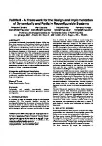
is typically a fixed number of days larger than Order-Date. Such a data set (250 tuples, requiring 750 values of storage) is depicted in Figure 1: the values for Order-Date were generated uniformly within the interval [1, 500], the values for Ship-Date uniformly within [Order-Date, Order-Date + 10]. Figure 2 (spline synopses) and Figure 3 (MHIST histogram) show the approximation of the data using 30 values of storage space. As a measure of the amount of correlation present between the attribute values of 2 attributes R.A1 , R.A2 , we use the Spearman rank-order correlation coefficient [31] rs , which is defined as follows. Let Ri be the rank of the value of attribute A1 in the i-th tuple, Si be the rank of the value of attribute A2 in ¯ S¯ the the i-th tuple (in case of ties, we use the appropriate midrank ), and R, corresponding average rank. Then the linear correlation coefficient of the ranks is defined as P|T | ¯ ¯ i=1 (Ri − R)(Si − S) q rs = qP . (2) P|T | |T | 2 2 ¯ ¯ i=1 (Ri − R) i=1 (Si − S) The linear correlation coefficient of the example distributions is rs = 0.88, the approximate distributions have values of rs = 0.83 (spline synopses) and rs = 0.99, corresponding to the intuitive interpretation of the figures. Preserving this type of correlation is crucial for a large number of queries, as the conditions specifying the inclusion/exclusion of attribute values generally depend on the attribute-value distribution. For example a query checking for delayed deliveries: SELECT ∗ FROM R1 WHERE R1 .Ship-Date − R1 .Order-Date > 20. would return no tuples on the original data, few in case of the spline synopses and very many for histogram-based approximation. Most approximation techniques are geared towards preserving the correlation between attribute value and the corresponding frequency, but disregard correlation between attribute values. 500

500

""

400

300

200

100

""

450

450

400

400

350

350

300

300

250

250

200

200

150

150

100

100 50

50

0 50

100

150

200

250

300

350

400

450

Fig. 1. Original Data

2.5

500

50

100

150

200

250

300

350

400

Fig. 2. Spline Synopsis

450

0

50

100

150

200

250

300

350

400

450

Fig. 3. MHIST Histogram

The Error Model

Our goal is to minimize the estimation error over all queries Qj ∈ Q. First consider a scenario in which all queries only depend on a single synopsis S0

500

over the data distribution T = {(v1 , f1 ), (v2 , f2 ), . . . , (vn , fn )}. We define the error for a given query Qj ∈ Q by characterizing how well the query result Result(Qj ) ⊆ T is approximated. Then we define the error over all queries in Q with respect to a data distribution T as ´ X X ³ (3) Error(Q, S0 ) := (fi − fˆi )2 + r · (kvi − vˆi k)2 Qj ∈Q

i∈{k|vk ∈Result(Qj )}

′

Thus, if we define wi := |{Q | vi ∈ Result(Q′ ), Q′ ∈ Q}|, the sum of the errors for each query posed to synopsis S0 can be written as : |T | X Error(Q, S0 ) := wi · (fi − fˆi )2 + r · wi · (kvi − vˆi k)2 . (4) i=1

Except for the weights wi , this is the error function (equation 1) minimized by spline synopses. Since the weights wi can be easily incorporated into the spline construction process, minimizing the query error in the case of a single distribution has become a problem of constructing the optimal spline synopsis, which has been solved in [23]. This is a slight simplification as it ignores approximation errors with regard to the boundary conditions of a query: when using a synopsis for answering a query some attribute values vˆi may be included in the approximate answer even though the corresponding vi would not be in the query result. Likewise, some attribute values may be erroneously excluded. In a scenario with multiple synopses S := {S1 , . . . , Sl }, each query Qj is answered S (depending on M in(Qj )) by a synopsis in S. We use a mapping function map : 2{Att(R)|R∈R} 7→ {1, . . . , l} to assign each queried attribute combination to exactly one synopsis. We will describe how to obtain this mapping in Section 3.2. Note that this model assumes that queries over the same attribute combination are always mapped to the same synopsis (otherwise it would be necessary to store additional information on the mapping of specific queries, which would in turn compete for the memory available for synopses). Thus, the error over a set of synopses S := {S1 , . . . , Sl } is defined as: l X (Error({Qj ∈ Q | map(M in(Qj )) = i}, Si ). Error(Q, S) = i=1

Since the error of each synopsis Si is dependent on the memory size Size(Si ) of the synopsis, this is more accurately stated as: l X (Error({Qj ∈ Q | map(M in(Qj )) = i}, Si )) Error(Q, S) = min (Size(S1 ),...,Size(Sl ))∈Nl

i=1

(5) Pl under the constraint that i=1 Size(Sl ) is equal to the memory size M available for all synopses together. Thus the problem of optimizing the estimation error for the entirety of queries in the workload can be seen as a problem of selecting the optimal set of synopses and choosing their sizes.

3

Synopsis Selection and Memory Allocation

To illustrate the issues involved in our method consider a workload Q = Q1 ∪Q2 , Q1 containing no1 queries Q′ (i.e., queries of type Q′ whose fraction in the entire

workload is proportional to no1 ) with M in(Q′ ) = {{R1 .A1 }} and Q2 containing no2 queries Q′′ with M in(Q′′ ) = {{R1 .A2 }}. Then these can be answered by either (a) two synopses S{R1 .A1 } and S{R1 .A2 } over each single attribute, or (b) one synopsis S{R1 .A1 ,R1 .A2 } over the joint data distribution of R1 .A1 and R1 .A2 . Therefore, to compute the optimal error for the overall available memory M we have to evaluate Error for combination (b) nz }| { Error(Q) := min Error(Q, S{R1 .A1 ,R1 .A2 } ) ¡ ¢o min Error(Q1 , S{R1 .A1 } ) + Error(Q2 , S{R1 .A2 } ) Size(S{R .A } )∈N 1 1 Size(S{R .A } )∈N 1 2

|

{z Error for combination (a)

}

(with Size(S{R1 .A1 ,R1 .A2 } ) = M and Size(S{R1 .A1 } ) + Size(S{R1 .A2 } ) = M ) and keep track of the resulting synopses and memory partitioning. So we can characterize the problem of computing the optimal set of synopses (and the corresponding memory allocation) as a two-step process: (1) Computing Error(Q′ , Sx ) for all candidate synopses Sx and all possible combinations of queries Q′ ⊆ Q that may be mapped to Sx and the maximum amount of Memory M to be used for Sx . This requires O(M · |Tx |2 ) steps (for optimal partitioning, see [23]) for each pair of Sx and Q′ and also generates the values of Error(Q′ , Sx ) for all values of Size(Sx ) ≤ M . (2) Selecting the optimal set of synopses from a set of candidates computing an optimal memory partitioning such that the weighted sum over all synopsis errors (weighted by the number of times each synopsis is queried) becomes minimal for the synopses included in the optimal solution. Since the weights change according to the combinations of synopses in the solution, this is a different and more difficult problem than finding the optimal combination of synopses for different relations (which was solved by dynamic programming in [23]). As we will see in Section 3.2, the problem of synopsis selection and memory partitioning are closely related and thus solved together. In the following (Sections 3.1 and 3.2), we will show how to solve the above problem for a single dataset R ∈ R. The sub-solutions for all datasets in R can then be combined to solve the overall problem (Section 3.3). 3.1

Pruning the Search Space

Note that in the above example we never considered the combinations S ′ = {S{R1 .A1 } , S{R1 .A1 ,R1 .A2 } } or S ′′ = {S{R1 .A2 } , S{R1 .A1 ,R1 .A2 } }. This is due to a simple property of spline synopses, which also normally holds for both histograms and Wavelet-based approximations:

Observation 1, ”Pruning Property”: When answering queries over the set of attributes a, a synopsis Sx , over the set of attributes x with a ⊆ x will yield more accurate answers than a synopsis Sy if x ⊂ y and both synopses are of identical size. While artificial data distributions can be constructed that do not obey the above observation, we have found the pruning property to hold in all experiments on real-life datasets. The intuition behind it is the fact that by including more attributes in a synopsis, the number of unique attribute-value combinations vi in the corresponding data distribution increases as well (in this respect, the synopsis selection problem is similar to the one of index selection), making it harder to capture all attribute values/frequencies with acceptable accuracy. In the above case, it means that S{R1 .A1 } answers queries posed to R1 .A1 better than S{R1 .A1 ,R1 .A2 } (using the same memory). Similarly S{R1 .A2 } is an improvement over S{R1 .A1 ,R1 .A2 } for queries posed to R1 .A2 . Thus the combination S = {S{R1 .A1 } , S{R1 .A2 } } generally outperforms S ′ or S ′′ . Using the above observation, it becomes possible to characterize the set of candidate synopses in a compact manner. Consider a single relation R. Then the sets of attributes of R queried is Syn(R, Q) := {M in(Qi ) | Qi ∈ Q}. Now the set of all candidate synopses for R can be defined as: [ Cand(R, Q) := {Sx | x = z, z ⊆ Syn(R, Q)} This means that the set of all candidate synopses forms a lattice over the attribute-combinations queried; e.g. if Syn(R, Q) = {{R.A1 }, {R.A2 }, {R.A2 , R.A3 }, {R.A3 }} then Cand(R, Q) = {{R.A1 }, {R.A2 }, {R.A3 }, {R.A1 , R.A2 }, {R.A1 , R.A3 }, {R.A2 , R.A3 }, {R.A1 , R.A2 , R.A3 }}. The intuition behind the definition of Cand(R, Q) is the following: if a Synopsis Sy is in Cand(R, Q), it must be considered, for it is the most efficient way to answer a subset of queries of R using only one synopsis (all other synopses capable of answering the same subset would be less efficient, due to the pruning property). Conversely, if SSy 6∈ Cand(R, Q) then y must be of the form y = cand ∪ nocand withScand ∈ { z, z ⊆ Syn(R, Q)}, nocand ⊆ Att(R), ∀x ∈ nocand : (cand ∪ x) 6∈ { z, z ⊆ Syn(R, Q)}. But then Scand answers the same set of queries as Sy and does so more efficiently, since cand ⊂ y. We further utilize a second observation for further pruning of the search space. Observation 2, ”Merge Property”: For a set of queries Q each querying the same combination of attributes A, the error for answering the queries using one synopsis S over A with M memory is smaller than the error using two synopses S1 , S2 over A, which together use memory M . The intuition for this property is the following: By joining the synopses S1 and S2 , the estimation for the (potentially) overlapping regions in S1 and S2 is improved, as additional memory is invested in its estimation. It is a trivial consequence that the merge property also holds for combinations of more than two synopses over A. In contrast to the pruning property, it is possible to prove that the merge property always holds (see appendix A for the proof).

Because both of these properties typically apply also to approximation by histograms or wavelets, the following results also apply to the physical design problem when these techniques are used as base synopses1 . We do need to use a different error measure, however, as we cannot match corresponding tuples, because |Tx | is not invariant when approximated by either of these techniques. Instead, we suggest the use of an error measure that tracks the difference between the actual and the approximated data distribution, which computes its own matching, such as the MAC distance [18]. While its computation causes some additional overhead, it allows us to extend the results of this paper to virtually all approximation technqiues, which (a) satify both the Merge and the Pruning Property and (b) provide an approximation in the form of a data distribution, as defined in Section 2. 3.2

Selecting the Synopses for a Single Relation R

In the following we will describe, for a given set Q of queries over a single relation R, how to compute the optimal combination S of synopses, their sizes, and the corresponding mapping of queries, such that all queries can be answered and the overall error becomes minimal. As shown before, the optimal combination of synopses Sopt can consist of synopses over single attribute combinations from Syn(R, Q) that are optimal for a particular query in Q, as well as synopses for the joint attribute combinations of multiple members of Syn(R, Q), which are not optimal for any single query but more efficient than other combinations of synopses (using the same amount of memory) capable of answering the same queries. Now we want to capture this notion algorithmically, giving a method to construct a set of synopses for a given workload/data combination. We first introduce the necessary notation: Opt SynA,M := the combination of synopses for answering all queries over the attribute combinations in A ⊆ Syn(R, Q) using memory M as constructed below. Opt ErrA,M := the overall error resulting from Opt SynA,M . Now consider the problem of computing the optimal combination of synopses Opt SynA,M for given A and M . Opt SynA,M has one of the following forms: (a) Opt SynA,M = {SS A } with Size(SS A ) = M (one synopsis for all queries over the attribute combinations in A). (b) Opt SynA,M = Opt SynA′ ,m′ ∪ Opt SynA−A′ ,M−m′ (a combination of the optimal synopses for answering two disjoint subsets of A with A′ 6= ∅). Because of the merge property, we consider only decompositions for which Opt SynA′ ,m′ ∩ Opt SynA−A′ ,M −m′ = ∅. 1

Because both techniques generally only optimize the approximation of the attribute value this holds only with regard to the corresponding frequency error P|T | frequencies, ˆ 2 i=0 ((fi − fi ) .

Which combination is optimal depends on the error resulting from each alternative: [ In case (a) Opt ErrA,M = Error( {Q′ | M in(Q′ ) = A} , {SS A }) with {z } | Size(SS

A) = M . In case (b) Opt ErrA,M =

The set of queries answered by SS A

min

m′ ∈{1,...,M −1}

Opt ErrA′ ,m′ + Opt ErrA−A′ ,M −m′

Therefore, we can compute the optimal set of synopses for A by computing the minimal error for cases (a) and (b) and choosing the memory partitioning that minimizes the corresponding error. Note that by computing the optimal combination of synopses in the above manner, we implicitly also compute a mapping that dictates which attribute combinations from Syn(R, Q) are mapped to which synopses: because of the above decomposition, S := Opt ErrS Syn(R,Q),M is of the form S = {SS A1 , . . . , SS Al } with each a ∈ Syn(R, Q) being a member of exactly one A1 , . . . , Al . While more complex models are possible in which queries over the same attribute combination are mapped to different members of S, this would mean that additional information, from which the correct mapping for each single query could be derived at run-time, would have to be stored (creating contention for memory with the actual data synopses). Using the above definitions, the final set of synopses kept for R using memory M is Opt SynS Syn(R,Q),M , the corresponding error being Opt ErrS Syn(R,Q),M . However, it is still necessary to prove that the optimal solution can indeed be obtained based on the decompositions described above: Theorem: Opt SynA,M constructed in the above manner is the optimal combination of synopses for answering all queries in Q over the attribute combinations in A, when the pruning and merge properties hold. Proof: We show that S := Opt SynA,M using the above construction implies that S is the optimal combination of synopses answering all queries over the attribute combinations in A using memory M . This is proven by induction over |A|:

|A| = 1 : Then Opt SynA,M = {SA } (no partitioning involving multiple synopses possible because of the merge property), and because of the pruning property SA is the best way to answer queries over A. |A| → |A| + 1 : Now we assume that all Opt SynA,M for |A| ≤ h are indeed optimal and try to show the optimality for Opt SynA,M with |A| = h+1. This is shown by contradiction: Assumption: There exists a solution Sopt = {Sx1 , . . . , Sxt } (with Size(Sxi ) = mi , i = 1, . . . , t) such that the resulting overall error Erropt over all queries is indeed smaller than Opt ErrA,M with Sopt 6= Opt SynA,M . (Case 1) |Sopt | = 1 : Then Sopt = {SA′ }, with Size(SA′ ) = M . Since Sopt has a smaller Error than Opt ErrA,M , Sopt 6= {SA } (as SA is a possible synopsis combination for Opt SynA,M and thus Error(Q, {SA }) ≥

Opt ErrA,M > Erropt ). However, since Sopt must be able to answer all queries over A, A ⊂ A′ holds. Then it follows from the pruning property that Opt SynA,M results in better accuracy than Sopt , contradicting the previous assumption. (Case 2) |Sopt | > 1 : Because of the merge property, we assume that all queries to the same attribute combination a ∈ A are mapped to the same ′ , for which synopsis. Should this not be the case, we can replace Sopt by Sopt all synopses over the same attribute have been merged, resulting in a smaller ′ error. If we can now contradict the assumption for Sopt , we thereby contradict it for Sopt , too. Now Sopt can be written as Sopt = S1 ∪ S2 , S1 6= ∅, S1 6= S, S2 := S − S1 with S1 = {Sx11 , . . . , Sx1p }, S2 = {Sx21 , . . . , Sx2q }, p ≤ h, q ≤ h. Because all queries over the same attribute combination are mapped to the same synopsis , both S1 and S2 each answer queries over the attribute combinations in disjoint subsets A1 , A2 of A with A1 ∪ A2 = A. Then it follows from the induction hypothesis that Opt SynA1 ,P pi=0 Size(Sx1 ) results in a smaller error than S1 i

for queries over attribute combinations in A1 , and Opt SynA1 ,P qi=0 Size(Sx1 ) i

results in a smaller error than S2 for queries over attribute combinations in A2 . It follows that the error for OptA,M is less than the one caused by Sopt , contradicting the assumption. ⊓ ⊔ 3.3

Selecting the Synopses for all Relations

The error over all relations for total memory size M can now be written as Error(Q, S) =

min

(M1 ,...,M|R| )∈N|R|

|R| X i=1

Opt ErrS Syn(Ri ,Q),Mi

(6)

P|R| under the constraint that i=1 Mi = M . Note that this is equivalent to the initial definition in equation 5. Expression 6 can be solved by dynamic programming using O(M 2 · |R|) operations. By keeping track of the memory partitioningS(M1 , . . . , M|R| ), we can then determine the optimal set of synopses Opt SynS Syn(Ri ,Q),Mi . S := i=1,...,|R|

3.4

Reducing the Computational Overhead

So computing the optimal set of synopses S for a given query Q can be broken down into three steps: (1) Computing the error for each candidate synopsis and each combination of queries. (2) Computing the optimal set of synopses for each relation Ri ∈ R and all possible values Mi for the allocated memory. (3) Solving equation 6 to determine how much memory to dedicate to each relation’s synopses. Only step 3 is of low computational overhead, while steps 1 & 2 are expensive even for small instances of Syn(R, Q). This means that while our method scales up well with a rising number of relations, we need to ensure the tractability of the computation of Opt SynS Syn(R,Q),M for relations

in which many different attribute combinations are being queried (recall that our potential application domains include data mining tasks on datasets that may have dozens of attributes, and we also consider virtual relations for join synopses). We address potential bottlenecks for both step 1 and 2 for a single relation R in the following sections. Computation of the Error Values Before computing Opt SynS Syn(R,Q),M for a given relation R, it is necessary to compute Error(Q′ , Sx ) for Size(Sx ) ranging from 1 to M , for all Sx ∈ Cand(R, Q) and all combinations of queries Q′ ⊆ Q that can be answered by Sx in our model (i.e., all combinations of queries corresponding to disjoint attribute combinations ⊆ x). Computing each Error(Q′ , Sx ) means constructing the corresponding synopsis with memory M and requires O(|Tx |2 · M + M 2 ) operations (because the construction process computes Error(Q′ , Sx ) for all Size(Sx ) < M at no additional cost, we only need to construct the synopsis once). It follows that we can address this potential bottleneck by either reducing the number of combinations of x and Q′ considered or by reducing the complexity of computing each Error(Q′ , Sx ), i.e., of constructing the corresponding synopsis. Reducing the number of x, Q′ combinations: We can significantly reduce the number of combinations under consideration by assuming that all future queries are equally likely to access a given (multidimensional) attribute-value region in the synopsis. This would mean that instead of minimizing the weighted error in equation 4, all weights would be uniformly set to wi := 1. So the workload information in Q is then used to obtain how often certain attribute combinations are queried, but we do not use any information on query locality with regard to attribute values. This furthermore makes it possible to maintain large traces of previously executed queries without using significant memory, for now only the number of queries to each synopsis have to be tracked. Note that we only make this simplification when computing the Error values used for determining the combination and size of the synopses stored. Locality information (if collected) can still be used when computing the final synopses themselves. Under this assumption, we only have to compute Error(Q′ , Sx ) once for each x. Q′ then corresponds to the set of all possible queries on Sx . Thus the number of different synopses to compute would be given by |Cand(R, Q)| (we will discuss methods for reducing |Cand(R, Q)| in Section 3.4). Also Error(Q′ , Sx ) with Size(Sx ) = M can now be characterized as Error(Q′ , Sx ) = |Q′ | · error for approximating Tx in M memory. ′

= |Q | ·

|T | X i=1

(fi − fˆi )2 + r · (kvi − vˆi k)2

This approach also allows the Error values to be computed lazily (i.e., whenever the underlying database system, data-mining or mediation platform has free resources) and stored until the corresponding datasets change significantly. We

refer to this heuristic as Uniform-Locality. Reducing the overhead of synopsis construction: The overhead caused by this part of the algorithm can be reduced significantly, by (initially) not using the optimal algorithm when generating synopses, but using faster and less accurate heuristics. With spline synopses, the computational overhead for computing a single synopsis Sx can be reduced from O(|Tx |2 ·M +M 2 ) to O(|Tx |· log2 |Tx | · M + M 2 ), leading to a dramatic decrease in the actual running times (for measurements, see [23], Section 6). The important, empirically observed, feature here is that the loss in accuracy is relatively uniform for all candidate synopses, resulting in Error values that lead to a synopsis set S ′ very close to the optimal set S. A similar approach is possible using histograms; an approximate algorithm for partitioning V-Optimal histograms can be found in [20]. After S has been selected, the final synopses in S can be (re-)computed using the optimal algorithm; the resulting overall running time is significantly shorter S Cand(Ri , Q)| ≫ |S|. We refer to this heuristic than before, since generally | i=1,...,n

as Greedy-Construction. Reducing |Cand(R, Q)| With the modifications of the previous subsection, the overhead of both step 1 & 2 in the construction of the (near-)optimal synopses is determined by the size of the set of candidate synopses Cand(R, Q):

In step 1 we have to construct |Cand(R, Q)| synopses to obtain the resulting Error values, and

in step 2, Cand(R, Q) is crucial to limit the number of different combinations of attributes A′ , A−A′ examined in sub-case (b) of the construction of Opt Syn. Therefore, we consider merely a small number of “promising” attribute combinations for synopses in Cand(R, Q). The key to finding such promising attribute combinations is to be able to “guess” the resulting Error values with reasonable accuracy without having to actually compute them. We found during our experiments with multidimensional spline synopses, that |Tx | is a good indicator regarding the size of the resulting approximation error, i.e., if |Tx | < |Ty | then typically Error(Q′ , Sx ) < Error(Q′ , Sy ) when Size(Sx ) = Size(Sy ). Intuitively, utilizing this rule means assuming that all data distributions are “equally difficult” to approximate and thus the resulting approximation error depends on the size of the data distribution. Based on these considerations we choose the set of “promising” synopses \ Cand(R, Q) in the following way. Initially, for each synopsis Sa ∈ Syn(R, Q), we \ add Sa to Cand(R, Q), as it is the best way to answer queries over the attribute combination a only. For the remaining synopses Sa ∈ Cand(R, Q) we compute |Tx | ′ val(x) := |Q ′ | , with Q being the number of queries in Q for which Sa can be \ used. We then include the 2 · |Att(R)| synopses Sy in Cand(R, Q) corresponding to the lowest values for val(y). In the following, we will refer to this heuristic as Small-Cand.

4

Putting the Pieces Together

Solving the physical design problem for data synopses can be characterized as a 4-step process: 1) Collection of workload information: We first need to acquire the necessary information about the access behavior of the workload, which can be done automatically by the data manager that processes the queries. The details of this information depend on the heuristics we employ for solving the physical design problem: when assuming that all data points of a table are equally likely to be accessed (Small-Cand, see Section 3.4), we only need to collect the access frequency of each attribute combination present in the workload. Otherwise, we also need to store the access frequencies for attribute value combinations; however, this is only necessary for tables that are both very important (e.g., resource-intensive) and exhibit significant locality in their access behavior. 2) Enumeration of all possible synopsis combinations: As described in Section 3.3 the synopses selection problem can be solved for each relation independently; from the resulting sub-solutions the overall combination can then be obtained by solving equation 6. To obtain the sub-solution for each relation Ri ∈ R, we first compute all possible synopsis combinations for Opt SynA,M for Ri . This is done by traversing the lattice of the attribute combinations in Cand(Ri , Q) in the order of the sizes |Tx | of the data distributions at each node. For each node we compute all synopsis combinations possible from its attribute combinations Ai and all subsets of Ai corresponding to nodes in the lattice (as well as potential mappings from queries to synopses). 3) Minimization of the error values: As described in Section 3.2, each of the combinations of synopses and mappings corresponds to an Opt Err expression, which is defined in the form of a minimization problem. In order to determine the best synopsis combination, we have to compute the corresponding values for Opt Err. This is done by constructing the corresponding synopses and evaluating the error for the resulting data distributions. The minimum Opt Err expression corresponds to the optimal synopsis combination. By alternating between enumeration and minimization, we can avoid solving similar minimization problems more than once. By combining the enumeration and minimization steps, it is furthermore possible to avoid solving identical minimization-problems more than once. Each time a new (sub-) combination of synopses/mapping is created the corresponding minimization problem is solved immediately. Because each new combination is either created by joining two previously know combinations together, plus at most one additional synopsis, the corresponding minimization problem can be solved using the solutions for the two joining synopses in at most O(M ) steps. 4) Construction of the final synopses: The overall optimal solution can now be obtained from the sub-solutions for each relation by minimizing equation 6.

The computational overhead of our techniques is caused by (a) the computation of the candidate synopses, (b) the solving of the resulting minimization problems, and (c) the enumeration of all possible minimization problems. A detailed discussion of the running times for (a) and (b) can be found in [23], including the cost of memory reconciliation and the tradeoffs connected with Greedy-Construction. In order to assess the cost of (c), enumerating all minimization problems, we had our algorithm construct all possible synopses for a given set of attributes A for which all possible subsets were queried (i.e. 2|A| different types of queries and thus the same worst-case number of potential synopses). The running times for this worst-case stress test are shown in Table 1. Obviously, even though the space of all combinations grows exponentially with the size of A, the enumeration is still reasonably efficient for up to 20 attributes, which covers the range of query-relevant attributes in most tables (including join views) in relational databases. We have also developed a number # Attributes Running time (sec.) # Attributes Running time (sec.) 4 0, 009 sec. 12 1, 23 sec. 8 0, 049 sec. 16 93, 93 sec. Table 1. Running times for the enumeration on a SUN UltraSPARC 4000 (168 Mhz)

of heuristic algorithms, that alleviate the potential bottlenecks arising from our approach. A detailed description of these can be found in the extended version of this paper [24].

5

Experiments

To validate our approach and to demonstrate both its accuracy and low overhead, we have implemented our techniques and applied them to a scenario based on the TPC-H decision support benchmark. We compared the synopses selection techniques introduced in this paper against several simpler heuristics. Because we are not aware of other approaches to the given problem, these heuristics are not intended to represent opponents. Rather, some represent assumptions commonly used in connection with synopses selection in commercial database systems. Others are used to examine how much approximation accuracy is affected by simpler approaches to either synopses selection or memory allocation. 5.1

Base Experiment

We used a subset of the queries of TPC-H , chosen to be large enough to make the synopses-selection problem non-trivial yet small enough to facilitate understanding of the resulting physical design. The queries selected were Q1 , Q6 , Q13 , Q15 and Q17 , referring to the Lineitem, Part, Orders, and Customer tables2 . 2

The non-numerical values present in a TPC-H database are coded as numbers. For example, P.Brand consists of a constant text string and two integers in the range [1, 5]. We only store the 25 possible number combinations.

Table 2 shows the query-relevant attribute sets, the minimum sets M in(Qi ), for the above five queries. We chose these minimum sets according to a result-size Query Q1 Q6 Q13 Q15 Q17

Min-Set L.Shipdate L.Shipdate, L.Discount, L.Quantity J1 .Extended price, J1 .Clerk, J1 .Discount, J1 .Return Flag L.Extended price, L.Shipdate, L.Discount J2 .Container, J2 .Discount, J2 .Quantity, J2 .Brand Table 2. The Mininmum Sets for the used queries

approximation scenario, i.e., we only selected those attributes that are necessary to estimate the number of tuples in the query results (for queries which have an aggregation as the last operator, we estimate the result-size before the aggregation). This results in five multidimensional data distributions. Three of these are projections of the Lineitem table, referred to as L onto subsets of its attributes (which all overlap so that there are a number of different, potentially suitable combinations of synopses). The other two data distributions to be approximated are join synopses J1 = Lineitem ⊲⊳ Orders and J2 =Lineitem ⊲⊳ Part. For our experiments, we used a scaled-down version of the TPC-H 1 data with scale factor SF= 100 ) and SF ∗ 500 KBytes memory available for all synopses together). We compared the physical design technique presented in this paper against six heuristic competitors that were generated from the following two option sets for synopses selection and memory allocation. Synopses selection: Single A single-dimensional synopsis was allocated for each attribute that appears at least once in the minimum sets of the five queries. While this heuristics cannot be expected to perform comparably to the more sophisticated allocation schema, we included it since most commercial database systems still use one-dimensional synopses/histograms only. So this heuristics gives an idea of the loss in accuracy when ignoring multi-attribute correlation. Table One multidimensional synopsis is allocated for each table, and this synopsis covers all attributes of the table that appear in the minimum sets. This heuristic results in a large single synopsis reflecting all correlations between attributes. However, because of the merge-property, the its accuracy may be significantly less than synopses using subsets of attributes. and Memory allocation: Uniform Each synopsis is given the same size. Again, this assumption can be found in commercial database systems. Tuples The size of a synopsis is proportional to the size of the table that it refers to, measured in the number of tuples that reside in the table (where a join result is viewed as a table, too) multiplied with the number of attributes covered by the synopsis.

Values The size of a synopsis is proportional to the size of the unique value combinations among the attributes over which the synopsis is built. The synopsis-selection technique of this paper is referred to as Opt Syn, the corresponding memory reconciliation as Opt Size. To illustrate the importance of memory reconciliation for our overall approach, we also combined our synopsisselection with the Uniform, Tuples and Values-based memory allocation; i.e., the optimal set of synopses was first generated and the sizes of these synopses were then computed using the above heuristics. For each set of synopses we executed 1000 instances of each query (using different, uniformly distributed, inputs for the query parameters, as specified in the benchmark) and used the available synopses to estimate the result sizes. We measured the average relative error of the result sizes: X |(exact size(i)−estimated size(i))| Relative Error := n1 exact size(i) i=1,...,n

with n being the number of instances of all queries together. All queries occur with the same frequency in all experiments. Regarding the heuristics introduced in Section 3.4, we did not use locality information when computing the optimal synopsis combinations or the final synopses; rather we did use the complete set of candidate synopses. The results of the first experiment are shown in the first three columns of Table 3. Selection Memory Original data Skewed data Query locality Single Uniform 1.98 7.98 10.19 Tuples 1.98 7.42 9.72 Values 1.92 7.62 9.34 Table Uniform 1.46 3.14 4.96 Tuples 1.47 3.17 5.11 Values 1.43 3.47 5.01 Opt Syn Uniform 1.05 1.14 1.04 Opt Syn Values 1.04 1.01 1.27 Opt Syn Tuples 1.03 1.08 1.17 Opt Syn Opt Size 1.04 0.83 0.85 Table 3. Error for the original TPC-H skewed and locally accessed data

In this set of experiments, our technique employed for synopses selection had significant impact on the resulting approximation accuracy, whereas the way memory is allocated only results in negligible changes to the overall error. 5.2

Skewed and Correlated Data

As described earlier, for purposes of approximation it is crucial to preserve the correlation contained in the data. Unfortunately, the original TPC-H data is generated using uniformly random distributions for each attribute, resulting in

almost completely uncorrelated data3 , which is not a good benchmark for data approximation techniques. Therefore, we ran a second set of experiments using the same schema, but with skewed and correlated data. This more realistic kind of data was generated the following way: Skew in attribute-value frequencies. We generated the attribute-value frequencies so that the frequency of the attribute values was Zipf-like distributed; i.e., the frequency of the i-th most frequent value is proportional to (1/i)θ where θ is a control parameter for the degree of skew. In this experiment we used θ = 1. Correlation between attributes Here we permuted the generated data in order to obtain the desired correlation. After creating the data according to the TPC-H specification, we then performed (randomly chosen) permutations on the values of selected attributes in order to create specific correlations between pairs of attributes. The correlation itself is specified in terms of the linear correlation coefficient rs [31]. For each of the following pairs of attributes we created data with a linear correlation coefficient rs ∈ [0.725, 0.775] : (L.Shipdate, L.Quantity),(J2 .Brand, J2 .Container), (P.Partkey, P.Brand). The results for this experiment are shown in the fourth column of Table 3. Again, the choice of the synopses-selection technique was most important with regards to the resulting approximation error: our Opt Syn technique developed in this paper reduced the error by a factor of 7 and 3 compared to the Single and Table heuristics, respectively. In addition, with Opt Syn for synopses selection, the use of our memory reconciliation technique Opt Size resulted in noticeable further improvement. So for this more realistic dataset, the combination of Opt Syn and Opt Size outperformed all competitors by a significant margin. 5.3

Query Locality

We repeated the above experiments using a workload that exhibited significant locality, again using the data exhibiting significant skew and correlation. For this experiment, we generated the input parameters for the TPC-H queries using a Zipf-like distribution (θ = 0.25), first executing 1000 queries of each type to obtain the weights wi (see equation 4) we then used to construct the synopses. Subsequently, we ran another 1000 queries (with different parameters generated by the same probability distribution) for which we measured the error. The results for this experiment are shown in the fifth column of Table 3. The trends from the previous experiment can be observed here as well: the synopses-selection technique clearly outperforms the simpler approaches, with the estimation accuracy further improving when memory reconciliation is used.

6

Conclusions

In this paper we motivated and defined the physical design problem for data synopses. We proposed an algorithmic approach to its solution, discussed heuristics 3

The exceptions being O.Totalprice (correlated with L.Tax, L.Discout, L.Extendedprice), L.Shipdate (correlated with O.Orderdate), L.Commitdate (correlated with O.Orderdate) and L.Receiptdate (correlated with L.Shipdate).

to alleviate computational bottlenecks, and provided an experimental evaluation. The experiments showed that the developed method achieves substantial gains over simpler heuristics in terms of the accuracy within the given memory constraint. They also showed that both aspects of our approach, synopses selection and tuning of the memory allocation, are important. Although we have carried out the derivation and implementation of our approach in the context of spline synopsis, our approach is orthogonal to the specific form of synopses and applies equally well to histograms as well as other techniques (with some minor modifications). We are working on a better theoretical foundation for the assumptions on which we have based our approach; e.g., there exist alternative partitioning techniques for both traditional histograms as well as spline-synopses that result in synopses obeying the Merge Property; unfortunately, the corresponding partitioning techniques have proven untractable. Future work will include exploring the use of Principal Component Analysis as a dimensionality reduction technique to exploit situations when two or more attributes are highly correlated or, in the extreme form, functionally dependent. We are also working on a better theoretical foundation for the pruning property assumption. These are in no way critical for the practicality of the developed method, but we wish to extend our overall framework and characterize optimality conditions in a precise manner.

A

Proof of the Merge Property

Claim: For a set of queries Q over the same attribute combination A, the error for answering these queries by a single synopsis Sunion is less to or equal to the error for Q with two synopses S1 , S2 , which together require the same amount of memory as Sunion . Proof: In Section 2.5 we showed that the error for a set of queries corresponds to the error of the fitting-problem posed in Equation 4. Therefore, if we can show that the value for Equation 4 is smaller for Sunion than for S1 and S2 , we have proven the overall statement. This will be done in the following manner: Based on a given S1 , S2 and Q we will construct a corresponding Sunion in terms of the bucket-partitioning used for fitting attribute frequencies and values. We will show that the overall error is less or equal for Sunion ; now, since our partitioning method for constructing spline synopses traverses the space of all possible partitionings, either Sunion or a synopsis with better overall error will result from running the spline synopses construction on Q. First, it is necessary to consider the storage requirements for spline synopses: buckets for both frequency- and attribute-value approximation store 3 values (each storing the leftmost attribute-value in the bucket and the fitting parameters); in addition, we have to store the following bookkeeping information to construct a directory of all synopses: (a) the relation approximated by the synopsis, (b) the combination of attributes approximated by the synopsis (coded as a bit-vector), (c) the total number of buckets, (d) the number of buckets used

for frequency-approximation, (e) the highest attribute-value stored in the synopsis/relation and (f) a pointer to the synopsis itself. This requires a total of 6 values storage for bookkeeping information. Therefore, each synopsis requires 6 + 3 · (number of buckets) of storage. Because we do not keep any further bookkeeping information, it is necessary to require that each synopsis approximates all values between the lowest and highest value stored. Otherwise it would not be possible to decide whether at run-time whether a query can be approximated by a synopsis or not, for the incoming queries may not be part of the workload the synopses were constructed over. i reWe also need to introduce the following notation: Define PTF Err as the spective error for the problem of fitting the frequencies (i.e. i=0 wi ·(fi − fˆi )2 ) in Phigh−1 i as i=low wi · (fi − fˆi )2 Synopsis Si . Define the constraint error F Err[low,high) i analogously, only with regard to fitfor Si . Define D Erri and D Err[low,high) ting of the attribute-values. Define Ii = [vstarti , vendi ) as this interval of the values approximated by Si . If I1 and I2 overlap, it has to be decided to which synopses to map the (parts of) queries in Q querying I1 ∩ I2 . As it is not possible to map every single query to a synopsis individually without introducing additional information, each query (part) querying the interval I1 ∩ I2 is mapped to the synopsis with the lower overall error in the area of intersection. Without loss of generality we assume that vstart1 ≤ vstart2 . For purposes of approximation, the each interval Ij is partitioned into buckets; we define a partitioning into k buckets as a k − tuple P = (low1j , . . . , lowkj ) corresponding to the buckets [vlowj , vlowj ), . . . , [vlowj , vendj ). 1

2

k

Now, given synopses S1 using b1 buckets (of which bf1 are used for frequencyapproximation)and S2 , using b2 buckets (bf2 defined analogously), we construct Sunion with at most b1 + b2 + 2 buckets, requiring the same amount of memory (as we incur the bookkeeping overhead only once, which allows us to keep the two additional buckets). Regarding the construction, we have to differentiate 3 scenarios: I1 ∩ I2 = ∅: In this case, we can construct Sunion on the union of the buckets in S1 and S2 , as there is no overlap between them. In order to fulfill the requirement of synopses approximating all values in the interval [vstart1 , vend2 ), we need to add two additional buckets (one for frequency, the other for attributevalue approximation) covering [vend1 , vstart2 ). Since these aren’t queried, however, this doesn’t influence the resulting error. Therefore Error(Q, Sunion ) = ⊔ F Err1 + F Err2 + D Err1 + D Err2 = Error(Q1 , S1 ) + Error(Q2 , S2 ).⊓ I1 ∩ I2 6= ∅, I1 ∩ I2 6= I1 , I1 ∩ I2 6= I2 : In this case, we first construct the frequency approximation of Sunion using at most bf1 + bf2 buckets. Here we have to differentiate 2 cases: (a) F ErrI11 ∩I2 ≤ F ErrI21 ∩I2 (*): Denote the partition for the frequency-approximation in S1 by P1f = (low11 , . . . , lowb1f ), for S2 P1f = (low12 , . . . , lowb2f ). Let k be 1

2

the smallest index such that vlowk2 > vend1 . If bf2 > 1, such a k must exist and we construct the partitioning for frequency-approximation in Sunion as

P = (low11 , . . . , lowb1f , end1 , lowk2 , . . . , lowb2f ). Otherwise (if bf2 1

= 1), the

2

(low11 , . . . , lowb1f , end1 ).

partitioning constructed is P = 1 In both cases, the corresponding frequency-approximation is Sunion has at f f most b1 + b2 buckets. The corresponding error for fitting the frequency2 values is F Errunion = F Err1 +F ErrI11 ∩I2 +F Err[end ≤ F Err1 + 1 ,end2 ) 2 2 1 2 F ErrI1 ∩I2 + F Err[end1 ,end2 ) = F Err + F Err (because of (*)). (b) F ErrI11 ∩I2 > F ErrI21 ∩I2 : In this case, the proof is analogous, with k defined as the largest index, such that vlowk1 ≤ vstart2 and P = (low11 , . . . , lowk1 , low12 , . . . , lowb2f ) (if bf1 = 1 then P = (low11 , low12 , . . . , lowb2f )). In this case F Errunion = 2

2

2 1 2 F ErrI21 ∩I2 +F Err[start ≤ F Err2 +F ErrI11 ∩I2 +F Err[start = F Err+ 1 ,start2 ) 1 ,start2 ) F Err1 + F Err2 .

The attribute-value approximation of Sunion can now be constructed similarly, yielding a synopses with b1 +b2 buckets, with Error(Q, Sunion ) ≤ F Err1 + F Err2 + D Err1 + D Err2 = Error(Q1 , S1 ) + Error(Q2 , S2 ).⊓ ⊔ I1 ∩ I2 = I2 : Again we have to separate two cases:

1 1 2 2 +D Err[start ≤ F Err[start +D Err[start : (a) F Err[start 1 ,end1 ) 1 ,end1 ) 1 ,end1 ) 1 ,end1 ) in this case we simply include all buckets in S1 into Sunion . Then Error(Q, S) = 1 1 +D Err[start ≤ F Err1 +D Err1 + F Err1 +D Err1 +F Err[start 1 ,end1 ) 1 ,end1 ) 2 2 F Err[start2 ,end2 ) + D Err[start2 ,end2 ) = Error(Q1 , S1 ) + Error(Q2 , S2 ). (b) Otherwise we again have to construct a new partitioning for both frequency and density-approximation such that F Errunion ≤ F Err1 + F Err2 and D Errunion ≤ D Err1 + D Err2 , using at most b1 + b2 + 2 buckets. For the frequency-approximation in Sunion this is done in the following way: denote the partition for the frequency-approximation in S1 by P1f = (low11 , . . . , lowb1f ), 1

for S2 by P1f = (low12 , . . . , lowb2f ). Now define k as the number of buckets in 2

S1 such that vlowi < vstart2 , define k ′ as the number of buckets in S1 such that vlowi ≥ vend2 . Then we construct P = (low11 , . . . , lowk1 , low12 , . . . , lowb2f , 2

end2 , lowk1′ , . . . , lowb1f ). This results in k + 1 + bf2 + (bf1 − k ′ + 1) buckets, 1

which is at most bf1 + bf2 + 1, since k ′ − k ≥ 1. The resulting error for ap1 proximation of value frequencies if F union = F Err[start + F Err2 . 1 ,start2 ) The construction for the attribute-value approximation is similar. ⊓ ⊔

References 1. S. Acharya, P. B. Gibbons, V. Poosala, and S. Ramaswamy. Join Synopses for Approximate Query Answering. In Proceedings of the ACM SIGMOD Conference, pages 275–286. ACM Press, 1999. 2. B. Blohsfeld, D. Korus, and B. Seeger. A Comparison of Selectivity Estimators for Range Queries on Metric Attributes. In Proceedings of the ACM SIGMOD Conference, pages 239–250, 1999.

3. A. Caprara, M. Fischetti, and D. Maio. Exact and approximate algorithms for the index selection problem in physical database design. TKDE, 7(6):955–967, 1995. 4. K. Chakrabarti, M. N. Garofalakis, R. Rastogi, and K. Shim. Approximate query processing using wavelets. In Proceedings of 26th International Conference on Very Large Data Bases, Cairo, Egypt, pages 111–122, 2000. 5. S. Chaudhuri. An overview of query optimization in relational systems. In Proceedings of ACM PODS Conference, pages 34–43, 1998. 6. S. Chaudhuri, R. Motwani, and V. R. Narasayya. On Random Sampling over Joins. In Proceedings of the ACM SIGMOD Conference, pages 263–274, 1999. 7. S. Chaudhuri and V. R. Narasayya. Index merging. In Proceedings of the 15th International Conference on Data Engineering, 23-26 March 1999, Sydney, Austrialia, pages 296–303, 1999. 8. S. Chaudhuri and V. R. Narasayya. Automating Statistics management for Query Optimizers. IEEE Conference on Data Engineering, pages 339–348, 2000. 9. C. M. Chen and N. Roussoploulos. Adaptive Selectivity Estimation Using Query Feedback. In Proceedings of the ACM SIGMOD Conference, pages 161–172, 1994. 10. S. Choenni, H. Wagterveld, H. M. Blanken, and T. Chang. TOPYDE: a Tool for Physical Database Design. In 6. Conference on Database and Expert Systems Applications, pages 502–511, London,UK, 1995. 11. S. J. Finkelstein, M. Schkolnick, and P. Tiberio. Physical Database Design for Relational Databases. TODS, 13(1):91–128, 1988. 12. V. Ganti, M.-L. Lee, and R. Ramakrishnan. Icicles: Self-tuning samples for approximate query answering. In VLDB 2000, Proceedings of 26th International Conference on Very Large Data Bases, Cairo, Egypt, pages 176–187, 2000. 13. P. B. Gibbons, S. Acharya, Y. Bartal, Y. Matias, S. Muthukrishnan, V. Poosala, S. Ramaswamy, and T. Suel. Aqua: System and techniques for approximate query answering. Technical report, Bell Labs, 1998. 14. P. B. Gibbons and Y. Matias. New Sampling-Based Summary Statistics for Improving Approximate Query Answers. In Proceedings of the ACM SIGMOD Conference, 1998. 15. P. B. Gibbons and Y. Matias. Synopsis Data Structures for Massive Data Sets. In Symposium on Discrete Algorithms, 1999. 16. P. B. Gibbons, Y. Matias, and V. Poosala. Fast Incremental Maintenance of Approximate Histograms. In Proceedings of the 23rd International Conference on Very Large Databases, 1997. 17. P. J. Haas. Selectivity and Cost Estimation for Joins Based on Random Sampling. Journal of Computer and System Sciences, pages 550–569, 1996. 18. Y. E. Ioannidis and V. Poosala. Histogram-Based Approximation of Set-Valued Query-Answers. In Proceedings of 25th International Conference on Very Large Data Bases, pages 174–185, 1999. 19. H. Jagadish, H. Jin, B. C. Ooi, and K.-L. Tan. Global Optimization of Histograms. In Proceedings of the ACM SIGMOD Conference. ACM Press, 2001. 20. H. V. Jagadish, N. Koudas, S. Mutukrishnan, V. Poosala, K. Sevcik, and T. Suel. Optimal Histograms with Quality Guarantees. In Proceedings 24th International Conference on Very Large Databases, pages 275–286, 1998. 21. N. Kabra and D. J. DeWitt. Efficient mid-query re-optimization of sub-optimal query execution plans. In Proceedings of the ACM SIGMOD Conference, 1998. 22. A. K¨ onig and G. Weikum. Combining Histograms and Parametric Curve Fitting for Feedback-Driven Query Result-size Estimation. In 25th International Conference on Very Large Databases, 1999.

23. A. K¨ onig and G. Weikum. Auto-Tuned Spline Synopses for Database Statistics Management. 10th Int. Conference on the Management of Data, Pune, India, 2000. 24. A. K¨ onig and G. Weikum. A Framework for the Physical Design Problem for Data Synopses (extended version) available at: http://www-dbs.cs.uni-sb.de/. 25. J.-H. Lee, D.-H. Kim, and C.-W. Chung. Multi-dimensional Selectivity Estimation Using Compressed Histogram Information. In Proceedings of the ACM SIGMOD Conference, pages 205–214, 1999. 26. Y. Matias, J. S. Vitter, and M. Wang. Wavelet-Based Histograms for Selectivity Estimation. In Proceedings of the ACM SIGMOD Conference, pages 448–459, 1998. 27. F. Naumann and U. Leser. Cooperative Query Answering with Density Scores. In 10th International Conference on the Management of Data, Pune, India, pages 33–44, 2000. 28. F. Naumann, U. Leser, and J. C. Freytag. Quality-driven Integration of Heterogenous Information Systems. In Proceedings of 25th International Conference on Very Large Data Bases, September 7-10, 1999, Edinburgh, Scotland, UK, pages 447–458, 1999. 29. V. Pooosala and Y. E. Ioannidis. Selectivity Estimation Without the Attribute Value Independence Assumption. In Proceedings of the ACM SIGMOD Conference, Athens, Greece, 1997. 30. V. Poosala. Histogram-based Estimation Techniques in Database Systems. PhD thesis, University of Wisconsin-Madison, 1997. 31. W. Press, S. Teukolsky, W. Vetterling, and B. Flannery. Numerical Receipes in C. Cambridge University Press, 1996. 32. S. Rozen and D. Shasha. A Framework for Automating Physical Database Design. In 17th International Conference on Very Large Data Bases, September 3-6, 1991, Barcelona, Catalonia, Spain, pages 401–411, 1991. 33. E. Skubalska-Rafajlowicz. The Closed Curve Filling Multidimensional Cube, Technical Report no. 46/94. ICT Technical University of Wroclaw, 1994. 34. W. Sun, Y. Ling, N. Rishe, and Y. Deng. An instant and accurate Size Estimation Method for Joins and Selections in an Retrival-Intensive Environment. In Proceedings of the ACM SIGMOD Conference, pages 79–88, 1993. 35. J. S. Vitter and M. Wang. Approximate Computation of Multidimensional Aggregates of Sparse Data using Wavelets. In Proceedings 1999 ACM SIGMOD International Conference on Management of Data, June 1-3, 1999, Philadephia, Pennsylvania, USA, pages 193–204. ACM Press, 1999.