A General Framework for Encoding and Evolving

A General Framework for Encoding and Evolving Neural Networks Yohannes Kassahun1 , Jan Hendrik Metzen1 , Jose de Gea1 , Mark Edgington1 , and Frank Kirchner1,2 1

2

Robotics Group, University of Bremen Robert-Hooke-Str. 5, D-28359, Bremen, Germany German Research Center for Artificial Intelligence (DFKI) Robert-Hooke-Str. 5, D-28359, Bremen, Germany

Abstract. In this paper we present a novel general framework for encoding and evolving networks called Common Genetic Encoding (CGE) that can be applied to both direct and indirect encoding methods. The encoding has important properties that makes it suitable for evolving neural networks: (1) It is complete in that it is able to represent all types of valid phenotype networks. (2) It is closed, i. e. every valid genotype represents a valid phenotype. Similarly, the encoding is closed under genetic operators such as structural mutation and crossover that act upon the genotype. Moreover, the encoding’s genotype can be seen as a composition of several subgenomes, which makes it to inherently support the evolution of modular networks in both direct and indirect encoding cases. To demonstrate our encoding, we present an experiment where direct encoding is used to learn the dynamic model of a two-link arm robot. We also provide an illustration of how the indirect-encoding features of CGE can be used in the area of artificial embryogeny.

1

Introduction

A meaningful combination of the principles of neural networks and evolutionary computation is useful for designing agents that learn and adapt to their environment through interaction. One step towards achieving such a combination involves the design of a flexible genetic encoding that is suitable for evolving networks using both direct and indirect encoding methods. To our knowledge, CGE is the first genetic encoding that tries to consider both direct and indirect encoding of networks under the same theoretical framework. In addition to supporting both types of genetic encodings, CGE has some important properties that makes it suitable for encoding and evolving neural networks. The paper is organized as follows: First, a detailed review of work in the area of Evolution of Artificial Neural Networks (EANNs) is given. Next, a description of CGE is provided. We then present an experiment in learning the dynamic model of a two-link arm robot, and illustrate how CGE can be used for artificial embryogeny. After this, a comparison of CGE to other genetic encodings is made. Finally, some conclusions and a future outlook is provided. J. Hertzberg, M. Beetz, and R. Englert (Eds.): KI 2007, LNAI 4667, pp. 205–219, 2007. c Springer-Verlag Berlin Heidelberg 2007 

206

2

Y. Kassahun et al.

Review of Work in Evolution of Artificial Neural Networks

The field of EANNs can be divided into two major areas of research: the evolution of connection weights, and the evolution of both structure and connection weights. In the first area, the structure of neural networks is fixed before the evolution begins. In the second area, both the structure and the connection weights are determined automatically during the evolutionary process. Since the evolution of connection weights is not interesting in the context of this paper, we will give only a review to relevant work in the second area. For a detailed review of the work in the evolution of neural networks see Yao [19]. Angeline et al. developed a system called GNARL (GeNeralized Acquisition of Recurrent Links) which uses only structural mutation of the topology, and parametric mutations of the weights as genetic search operators [1]. The main problem with this method is that genomes may end up in many extraneous disconnected structures that have no contribution to the solution. The Neuroevolution of Augmenting Topologies (NEAT) [17] evolves both the structure and weights of neural networks. It starts with networks of minimal structures and increases their complexity along the evolution path. The algorithm keeps track of the historical origin of every gene that is introduced through structural mutation. This history is used by a specially designed crossover operator to match genomes which encode different network topologies. Unlike GNARL, NEAT does not use self-adaptation of mutation step-sizes. Instead, each connection weight is perturbed with a fixed probability by adding a floating point number chosen from a uniform distribution of positive and negative values. Kitano’s grammar based encoding of neural networks uses Lindenmayer systems (L-systems) [12] to describe the morphogenesis of linear and branching structures in plants [10]. Sendhoff et al. extended Kitano’s grammar encoding with a recursive encoding of modular neural networks [16]. Their system provides a means of initializing the network weights, whereas in Kitano’s grammar based encoding, there is no direct way of representing the connection weights of neural networks in the genome. Gruau’s Cellular Encoding (CE) method is a language for local graph transformations that controls the division of cells which grow into an artificial neural network [5]. The genetic representations in CE are compact because genes can be reused several times during the development of the network and this saves space in the genome since not every connection and node needs to be explicitly specified in the genome. Defining a crossover operator for CE is still difficult, and it is not easy to analyze how crossover affects the subfunctions in CE encoding since they are not explicitly represented. Vaario et al. have developed a biologically inspired neural growth based on diffusion field modeling combined with genetic factors for controlling the growth of the network [18]. One weak point of this method is that it cannot generate networks with recurrent connections or networks with connections between neurons on different branches of the resulting tree structure. Nolfi and Parisi have modelled biological development at the chemical level using a reaction-diffusion model [14]. This method utilizes growth to create connectivity without explicitly describing each

A General Framework for Encoding and Evolving Neural Networks

207

connection in the phenotype. The complexity of a structure that the genome can represent is limited since every neuron is directly specified in the genome. Other work in indirect encoding have borrowed ideas from systems biology, and simulated Genetic Regulatory Networks (GRNs), in which genes produce signals that either activate or inhibit other genes in the genome. Typical works using GRNs include those of Dellaert and Beer [4], Jakobi [7], Bongard and Pfeifer [3], and Bentley and Kumar [2].

3

Common Genetic Encoding (CGE)

A genotype in CGE is a sequence of genes that can take one of three different forms: a vertex gene, an input gene, or a jumper gene. A vertex gene encodes a vertex of a network, an input gene encodes an input to the network, and a jumper gene encodes a connection between two vertices. A particular jumper gene can either be a forward or a recurrent jumper gene. A forward jumper gene represents a connection starting from a vertex gene with higher depth1 and ending at a vertex with lower or same depth. A recurrent jumper gene represents a connection between two vertices with arbitrary depths. Depending on whether the encoding is interpreted directly or indirectly, the vertex genes can store different information such as weights wi ∈ R (e.g. when the encoded network is interpreted directly as a neural network) or operator type (e.g. when the encoded network is indirectly mapped to a phenotype network). A genotype g = [x1 , ..., xN ] ∈ G is defined as a sequence of genes xi ∈ X , where G is the set of all valid genotypes, and X = V ∪ I ∪ JF ∪ JR . V is a set of vertex genes, I is a set of input genes, and JF and JR are sets of forward and recurrent jumper genes, respectively. For a gene x and a genotype g = [x1 , . . . , xN ] we say x ∈ g iff ∃ 0 < i ≤ N : x = xi . To each vertex gene there is an associated unique identity number id ∈ N0 and to each input gene there is an associated label, where input genes with the same label refer to the same input. The set of identity numbers and the set of labels are disjoint. Each vertex gene xi stores a value din (xi ), which can be interpreted as the number of expected inputs (i. e., the number of arguments of xi ). A forward or a recurrent jumper gene stores the identity number of its source vertex gene. Two genes xi ∈ g1 and xj ∈ g2 are considered to be equal if the following condition is satisfied: (xi ∨ (xi xi = xj ⇔ ∨ (xi ∨ (xi

∈ V ∧ xj ∈ V ∧ xi .id = xj .id) ∈ I ∧ xj ∈ I ∧ xi .label = xj .label) ∈ JF ∧ xj ∈ JF ∧ xi .source id = xj .source id) ∈ JR ∧ xj ∈ JR ∧ xi .source id = xj .source id)

(1)

There are different functions defined on the genes of a genotype that can be used for determining properties of the genotypes during the evolutionary run. The first function v : X −→ Z defined as  1 − din (xi ), if xi ∈ V (2) v(xi ) = /V 1, if xi ∈ 1

For a formal definition of a gene’s depth, see Equation 6.

208

Y. Kassahun et al.

can be interpreted as the number of implicitly produced outputs (which is always 1) minus the number of expected inputs by the gene xi . This function allows us to define the sum K−1  v(xi ), (3) sK = i=1

where K ∈ {1, . . . , N + 1}. Note that this definition implies s1 = 0. Based on this, we define the set of output vertex genes as Vo = {xj ∈ g | xj ∈ V ∧ (si < sj ∀ i : 0 < i < j)}

(4)

and the set of non-output vertex genes as Vno = V − Vo . We consider a subsequence gl,m = [xl , xl+1 , . . . , xl+m−1 ] of g to be a l+m−1  subgenome of a genotype g if xl ∈ V and sl,m = v(xi ) = 1. Subgenomes are i=l

an important concept in CGE, because they make it possible to treat developed phenotype structures as a composition of phenotype substructures that correspond to the subgenomes, and because of this, they allow the genetic encoding to inherently support the evolution of modular neural networks. We can define a hierarchy-relationship between the genes in a genotype by the function parent : X −→ V ∪ ∅  ∅, if (si < sj ∀ i : 0 < i < j) parent(xj ) = . (5) xi , if si ≥ sj and sk < sj ∀ k : 0 < i < k < j From equations (4) and (5), it follows that for an output vertex gene xj , parent(xj ) = ∅. The output of a gene xj acts implicitly as an input for parent(xj ). The depth of a vertex gene is defined as the minimal topological distance (i.e. minimal number of connections to be traversed) from an output vertex of the network to the vertex itself, where the path contains only implicit connections. This is defined mathematically by the function depth : V −→ N  0 if parent(xj ) = ∅ depth(xj ) = . (6) depth(parent(xj )) + 1, otherwise Table 1 shows an example of a genotype encoding the neural network shown in Figure 1 along with the resulting values of the above-defined functions. We consider two genotypes g1 and g2 to be equivalent if and only if there is a one-to-one correspondence between them, i. e. ∀ xi ∈ g1 ∃ xj ∈ g2 : xi = xj ∧ parent(xi ) = parent(xj ), and ∀ xj ∈ g2 ∃ xi ∈ g1 : xi = xj ∧ parent(xi ) = parent(xj ). The equivalence criterion between two genotypes can be used to lessen the competing convention problem [15] that is encountered during the evolution of neural networks. A newly generated genotype is tested against all existing genotypes before it is added to the population. If there is an already existing equivalent genotype, the newly generated genotype will not be added to the population.

A General Framework for Encoding and Evolving Neural Networks

209

Fig. 1. An example of a valid phenotype with two output vertices (0 and 4), and three input vertices (x, y and z)

The following five criteria must be fullfilled for a genotype g = [x1 , ..., xN ] to be considered a valid genotype, i. e. g ∈ G: 1. Each vertex gene xi ∈ V must have at least one input: din (xi ) > 0. 2. There can be no closed loops of forward jumper connection genes in g. 3. There is no forward jumper gene whose source vertex depth is less than the depth of its target vertex. 4. For a gene xk ∈ g, sk < sN +1 , ∀ k ∈ {1, ..., N }. 5. For every xk ∈ g: parent(xk ) = ∅ ⇒ xk ∈ V. A vertex gene xi with din (xi ) = 0 has no input and would always yield the same result. Because of this, such a vertex is not allowed (criterion 1). The second and third criteria together guarantee that the evaluation of a phenotype in the direct encoding case or the development process of a phenotype in the indirect encoding case can be completed in a finite amount of time (i. e. there are no infinite loops). The last two criteria together ensure that the sum of outputs produced by all genes in g minus the sum of all expected inputs is equal to the number of outputs of the corresponding phenotype network. We denote the set of phenotypes represented by CGE genotypes with PCGE . The development function D : G −→ PCGE formalizes a process that creates for every valid genotype g = [x1 , ..., xN ] ∈ G a corresponding phenotype p ∈ PCGE . We have designed three kinds of genetic operators for the use in CGE: parametric mutation, structural mutation and structural crossover. The genetic operators to be used in CGE are designed so that the resulting genotypes they produce fulfill the 5 criteria stated above. A parametric mutation PA : G −→ G changes only the values of the parameters included in the genes (e.g. the weights wi ). The order of the genes in g and PA(g) remains the same. An example of a structural mutation operator ST : G −→ G that fulfills the above criteria is defined as follows: when ST operates on a genotype, it either inserts a recurrent jumper gene, or a subgenome after a vertex gene xi , and the number of inputs din (xi ) will be increased by one. The source vertex of a recurrent jumper can be chosen arbitrarily. The subgenome consists of a vertex gene xk followed by

210

Y. Kassahun et al.

Table 1. The phenotype in Figure 1 is encoded by the genotype shown in this table. For each gene xi of the genotype, the gene’s defined properties and the values of various functions which operate on the gene are summarized. In the allele row, V denotes a vertex gene, I an input gene, JF a forward jumper gene, and JR a recurrent jumper gene. The source row shows the id of the source vertex of a jumper gene and the parent row shows the id of the parent gene. gene allele id source label weight din v s parent depth

x1 V 0 0.6 2 -1 0 ∅ 0

x2 V 1 0.8 2 -1 -1 0 1

x3 V 3 0.9 2 -1 -2 1 2

x4 I x 0.1 1 -3 3 -

x5 I y 0.4 1 -2 3 -

x6 I y 0.5 1 -1 1 -

x7 V 2 0.2 4 -3 0 0 1

x8 JF 3 0.3 1 -3 2 -

x9 I x 0.7 1 -2 2 -

x10 I y 0.8 1 -1 2 -

x11 JR 0 0.2 1 0 2 -

x12 V 4 0.9 2 -1 1 ∅ 0

x13 JF 2 0.2 1 0 4 -

x14 V 5 1.3 2 -1 1 4 1

x15 I y 2.0 1 0 5 -

x16 I z -1.0 1 1 5 -

an arbitrary number M > 0 of inputs or forward jumper genes. The number of inputs din to xk is set to M and its depth is set to depth(xi ) + 1. The depth of the source vertex of a forward jumper gene connected to xk is not allowed to have a depth less than the depth of xk . A good example of a crossover operator CR : G × G −→ G that can be used with CGE is the operator introduced by Stanley [17]. This operator aligns two genomes encoding different network topologies, and creates a new structure that combines the overlapping parts of the two parents as well as their differing parts. The id’s that are stored in vertex and jumper genes, and the labels that are stored in input genes, are used to align genomes.

4

Properties of the Encoding

In this section, we list some of the properties of the genetic encoding that makes it suitable for evolving neural networks. Formal proofs of these properties are given in [9]. The first property given by Proposition 1 reinforces the fourth and the fifth criterion listed in Section 3. Proposition 1.  For a valid genotype g ∈ G, the number of expected inputs by all din (xi ) is equal to |(Vno ∪ I ∪ JF ∪ JR )|, i. e. the number vertex genes xi ∈g∧xi ∈V

of non-output vertex genes. The second property given by Proposition 2 relates the sum sN +1 = to the number of output vertex genes in a valid genotype.

N

i=1

v(xi )

Proposition 2. For g = [x1 , ..., xN ] ∈ G with N genes, sN +1 is equal to the number of output vertex genes |Vo | in g.

A General Framework for Encoding and Evolving Neural Networks

211

This property can be used as a checksum while performing an implicit evaluation of a direct encoded phenotype, or during the development process of an indirect encoded phenotype. The following three important properties of the genetic encoding make it suitable for evolving neural networks. Proposition 3. (Completeness of G with respect to D) Every valid phenotype p ∈ PCGE can be represented by a genotype, i. e. D is surjective: ∀ p ∈ PCGE ∃ g ∈ G : D(g) = p. This proposition conveys that for every valid phenotype, there is a valid genotype that represents this phenotype (with respect to the development function D). Proposition 4. (Closure of D) The development function maps every valid genotype to a valid phenotype: ∀ g ∈ G : D(g) ∈ PCGE . The closure of D guarantees the generation of genotypes whose evaluation strategy (in the case of direct encoding) or development process (in the case of indirect encoding) terminates in a finite amount of time. Proposition 5. (Closure of G under genetic operators) The set of genotypes G is closed under the mutation operators PA and ST : PA(g) ∈ G and ST (g) ∈ G ∀ g ∈ G. Furthermore, it is closed under the crossover operator CR: CR(g1 , g2 ) ∈ G ∀ g1 ,g2 ∈ G. Proposition 5 emphasizes that the genetic operators are designed so that their output genotypes satisfy the validity criteria listed in Section 3.

5

CGE for Direct Encoding Case

In the direct encoding case, the phenotypes which can be represented by the valid genotypes are defined as follows: each valid phenotype p ∈ PCGE is a directed graph structure p = (V, E) consisting of a set of vertices V and a set of directed edges E. The set of edges E is partitioned into two subsets: the set of forward connections EF , and the set of recurrent connections ER . For each p = (V, EF ∪ ER ) ∈ PCGE , the subgraph pF = (V, EF ) is always a directed acyclic graph (DAG). The set ER can be an arbitrary subset of V × V . The development function D : G −→ PCGE creates for every valid genotype g = [x1 , ..., xN ] ∈ G a corresponding phenotype p ∈ PCGE . In the direct encoding case, for each xi ∈ V, p contains exactly one vertex x ˆi , which has the same identity number as xi , and for each recurrent jumper gene xi , there is an edge e ∈ ER from a vertex whose id is equal to that of xi ’s source vertex id to the vertex in p whose id is equal to that of parent(xi ). In the same way, for each xi ∈ JF there is a corresponding forward connection in EF . For each xi ∈ I, EF contains a forward connection from the vertex having xi ’s label as id2 to the 2

There may be several labels possessing the same value for different input vertices, but for each unique label, there exists only one vertex in p whose id corresponds to that label.

212

Y. Kassahun et al.

vertex with the same id as parent(xi ). Additionally, there are connections in EF that are not explicitly represented in g. Each non-output vertex gene xi ∈ Vno has an implicit forward connection with its parent vertex parent(xi ). The evaluation function evaluates the developed phenotype p ∈ PCGE . D(g) can be interpreted as an artificial neural network in the following way: all input vertices of D(g) are considered as inputs of the network and all other vertices as neuron nodes. The vertices corresponding to an output vertex gene in g are the output neurons of the network. Each forward and recurrent connection causes the output of its source neuron to be treated as an input of its target neuron. Each ˆi be a neuron with incoming artificial neuron stores its last output oi (t− 1). Let x forward connections from the inputs x ˆ1 , ..., xˆk and the neurons xˆk+1 , ..., x ˆl , and ˆm . For an arbitrarily the incoming recurrent connections from neurons x ˆl+1 , ..., x chosen transfer function ϕ, the current output oi (t) of the neuron xˆi is computed using k l m    wj Ij (t) + wj oj (t) + wj oj (t − 1)), (7) oi (t) = ϕ( j=1

j=k+1

j=l+1

where the values of Ij (t) represent the inputs of the neural network. If the network has p inputs and q output neurons, we can define E as a function which takes the phenotype D(g) and p real input values, and produces q real output values, i.e. E : PCGE × Rp −→ Rq . A nice feature of CGE in the direct encoding case is that it allows an implicit evaluation of the encoded phenotype without the need to decode this phenotype from the genotype via D [8]. For this purpose, we consider the ordering of the genes in the CGE encoding to be inverted (i. e. from right to left) and evaluate it according to the Reverse Polish Notation (RPN) scheme, where the operands (input genes and jumper genes) come before the operators (vertex genes). 5.1

Exploitation and Exploration of Structures

The evolution of neural networks starts with the generation of the initial genomes. The complexity of the initial genomes is determined by the domain expert and is specified by the maximum depth that can be assumed by the genomes. It then exploits the structures that are already in the system. By exploitation, we mean optimization of the weights of the structures. This is accomplished by an evolutionary process that occurs at smaller time-scale. The evolutionary process at smaller time-scale uses parametric mutation as a search operator. An example of the exploitation process is shown in Figure 2. Exploration of structures is done through structural mutation and crossover operator. The structural selection operator that occurs at larger time-scale selects the first half of the structures (species) to form the next generation. Since sub-networks that are introduced are not removed, there is a gradual increase in the number of structures and their complexity along the evolution path. This allows the meta-level evolutionary process to search for a solution starting from a neural network with minimum structural complexity specified by the domain expert. The search stops when a neural network with the necessary optimal structure

A General Framework for Encoding and Evolving Neural Networks

Trajectory in weight space

213

t

t+1 w(Iy)

w(Ix)

w(N0)

Fig. 2. The weight trajectory of a genome while it is being exploited. The quantities t and t + 1 are time units with respect to the larger time-scale. The weights of the existing structures are optimized between two consecutive time units with respect to the larger time-scale. The point clouds at t and t + 1 show populations of individuals from the same structure.

that solves a given task is obtained. The details of the exploitation and exploration of structures can be found in [8]. 5.2

Learning the Dynamic Model of a Robot Manipulator

The purpose of this experiment is to demonstrate the flexibility of a CGE encoding in solving a learning task. We will illustrate how the modular property of the encoding can be exploited in solving a given task in a divide and conquer strategy manner. Given an initial state of a mechanical structure (i.e. displacements q(0) and velocities q(0) ˙ of the joints) and the time history of torques τ (t) acting at joints, the direct dynamic model allows one to predict the resulting motion q(t) in joint space. With this information and the direct kinematic model, a prediction of the trajectory x(t) in Cartesian coordinates can be performed. For our experiment, the two-link planar arm shown in Figure 3 was used. The dynamic equation of the two-link arm [11] is used to simulate the robot. The learning system can observe the initial state s(0) = [q(0), q(0)] ˙ and q(t) for t between 0 and 1 sec. For a given initial state s(0), the learning system sends the robot arm the torque pair (τ1 , τ2 ) for the time between 0 and 1 sec, and records the resulting motion parameters q1 (t) and q2 (t). For a given torque pair (τ1 , τ2 ), the resulting motion by polynomials of degree 4  parameters are approximated  given by q1 (t) = 4k=0 ak tk and q2 (t) = 4k=0 bk tk . The polynomial approximation allows the where the velocities are given 4 velocities to be directly calculated, 4 by q˙1 (t) = k=1 k ∗ ak tk−1 and q˙2 (t) = k=1 k ∗ bk tk−1 . The genotype that represents the solution g = [g1 , g2 ] is made up of two subgenomes g1 and g2 each representing the motion parameters. To get an idea of how the genotype look like, we will explain the the subgenome g1 in detail corresponding to the first

214

Y. Kassahun et al.

Fig. 3. A two-link planar arm robot used for our experiment

motion parameter q1 (t). The polynomial approximation of q1 (t) can be written as 4  ak tk = a0 + t(a1 + t(a2 + t(a3 + a4 t))), (8) q1 (t) = k=0

where each of the coefficients ai is represented by a neural network ˙ whose output can be computed by equation (7). If we introMi (τ1 , τ2 , q(0), q(0)) duce two additional vertex genes V ∗ and V + , which take the product and the sum of their arguments respectively, we can represent the polynomial approximation in CGE genotype easily. Table 2 shows the first subgenome g1 , where Mi is a subgenome dedicated to coefficient ai . Note that a subgenome Mi is assigned v(xi ) = 1 since the sum sl,m for a subgenome is always one. A depth is also assigned to the subgenome Mi since by definition subgenomes start with a vertex gene. Table 2. A genotype representing the first subgenome g1 gene allele id source label weight din v s parent depth

x1 V+ 0 2 -1 0 ∅ 0

x2 M0 1 -1 0 1

x3 V∗ 1 2 -1 0 0 1

x4 I t 1 -1 1 -

x5 V+ 2 2 -1 0 1 2

x6 M1 1 -1 2 3

x7 V∗ 3 2 -1 0 2 3

x8 I t 1 -1 3 -

x9 V+ 4 2 -1 0 3 4

x10 M2 1 -1 4 5

x11 V∗ 5 2 -1 0 4 5

x12 I t 1 -1 5 -

x13 V+ 6 2 -1 0 5 6

x14 M3 1 -1 6 7

x15 V∗ 7 2 -1 0 6 7

x16 I t 1 -1 7 -

x17 M4 1 0 7 8

The learning process evolves each subgenome Mi independently using the meta-level evolutionary process discussed in Section 5.1. For the exploitation of structures the CMAES [6] algorithm developed by Hansen and Ostermeier is used. The parameters of the evolutionary process are set as follows: (1) Torque

A General Framework for Encoding and Evolving Neural Networks

0.5

0.5 Actual value Predicted Value

0

0

−0.5

−0.5

Angle 1 (rad)

Angle 1 (rad)

Actual value Predicted Value

−1

−1.5

−1

−1.5

−2

−2

−2.5

−2.5

−3

215

0

0.1

0.2

0.3

0.4

0.5

0.6

0.7

0.8

0.9

1

−3

0

Time (s)

(a)

0.1

0.2

0.3

0.4

0.5

0.6

0.7

0.8

0.9

1

Time (s)

(b)

Fig. 4. Actual and predicted values for q1 (t). (a) q1 (t) for τ1 = 0.05, τ2 = 0.05, q1 (0) = 0, and q˙1 (0) = 0. (b) q1 (t) for τ1 = 0.05, τ2 = 0, q1 (0) = 0, and q˙1 (0) = 0.

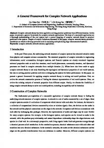
values are kept between -0.05 and 0.05 Nm. (2) Robot parameters are set to m1 = 0.05 Kg, m2 = 0.05 Kg, l1 = 0.25 m and l2 = 0.25m. (3) Crossover operator is turned off. (4) Structural mutation is turned on with probability 0.3 (5) Minimal initial structure for each subgenome Mi is set to have one output vertex gene connected to inputs τ1 , τ2 , q(0) and q(0). ˙ After learning the dynamic model of the robot, we tested it on unseen data. The performance of the learned model in predicting the motion parameters q1 (t) and q2 (t) is satisfactory. Figure 4 shows sample comparisons between actual and predicted values for q1 (t).

6

CGE for Artificial Embryogeny

The term embryogeny refers to the growth process which defines how a genotype maps onto a phenotype. Bentley and Kumar [2] identified three different types of embryogenies that have been used in evolutionary systems: external, explicit and implicit. External means that the developmental process (i. e. the embryogeny) itself is not subjected to evolution but is hand-designed and defined globally and externally to the genotypes. In explicit (evolved) embryogeny the developmental process itself is explicitly specified in the genotypes, and thus it is affected by the evolutionary process. Usually, the embryogeny is represented in the genotype as a tree-like structure following the paradigm of genetic programming. The third kind of embryogeny is implicit embryogeny, which comprises neither an external nor an explicit internal specification of the growth process. Instead, the embryogeny ”emerges” implicitly from the interaction and activation patterns of the different genes. This kind of embryogeny has the strongest resemblance to the process of natural evolution. A popular example of an implicit embryogeny is the Genetic Regulatory Network (GRN) [3,4]. In this section, we illustrate how CGE can be used to encode an explicit embryogeny. In explicit embryogeny schemes, a genotype contains a program that describes the developmental process. Most of these programs are represented as tree-like

216

Y. Kassahun et al.

structures, where each node of the tree contains an elementary instruction (like adding/removing an entity to the phenotype, conditional statements, iteration, a subroutine call, etc.) and (optionally) parameters for these instructions. During the development process, a tree is traversed (usually either in a breadth-first or depth-first manner) and the instruction contained in the current tree node is executed. Thus, while performing the tree traversal, the phenotype is grown stepby-step. Alternatively, the instructions can be contained in the edges of the tree and be carried out when the corresponding edge is traversed. This alternative is equivalent to the case in which instructions are contained in the nodes. For the following example, therefore, we consider only the case in which the instructions are contained in the nodes. For an encoding to be used for an explicit embryogeny scheme, it should possess the following features: (1) The encoding should be able to encode a tree structure. (2) A gene which encodes a node should contain an instruction as well as a set of parameters for this instruction. (3) The genetic operators must produce only offspring-genotypes which encode tree structures. Since the structures which can be encoded by a CGE-genotype are a superset of the set of all tree structures, one can fulfill the three conditions stated above by slight simplifications (modifications) of a CGE genotype. The first simplification is to do away with the need for input and jumper genes. In the original definition of CGE, each gene contains a weight. If CGE shall be used for explicit embryogeny, one must replace that weight by an arbitrary number of other parameters, which need not to be restricted to the domain of real numbers. The structural mutation operator must be changed in the following manner: instead of introducing recurrent jumper genes, forward jumper genes or input genes, it simply adds a new vertex gene in the genotype and increases the number of inputs of the vertex gene preceding the newly added gene. The parametric mutation operator itself remains largely unchanged - only the fields on which it operates are different: instead of modifying weights, it modifies now all parameters included in a gene, choosing the values from the domain which is associated with this kind of parameter. The crossover remains unchanged since it produces offspring which remains in the domain of tree structures. Kassahun et al. [9] have shown a way of encapsulating the edge encoding of Luke and Spector [13] into a CGE genotype. Thus, the basic ability of CGE to perform explicit (evolved) embryogeny has already been presented. However, since the edge encoding is an encoding scheme for neural networks, the phenotype remains in the domain of neural networks. In the following, we present a simple way of evolving phenotypes from other domains. For illustration purpose we use binary images I = {0, 1}128×128 as phenotypes. Each vertex gene of a genotype to be used contains one of the instructions {LEF T, RIGHT, U P, DOW N } and a binary parameter f ∈ {0, 1}. The growth process is as follows: Initially, all pixels of I are equal to 0 (i. e. white) and a virtual cursor points to the pixel with coordinates x = 0, y = 0. Then, a depth first traversal is performed and the instructions are executed as follows: If the instruction is LEF T , set x = x − 1 MOD 128 and I[x][y] = f . If the instruction is RIGHT , set x = x + 1 MOD 128

A General Framework for Encoding and Evolving Neural Networks

217

Fig. 5. The figure shows a genotype and the corresponding phenotype showing the letters ”KI”. The genotype is shown as a tree-like structure, which can be easily represented as a string of genes if the tree is traversed in a depth-first manner. The value of f is shown in parentheses. The phenotype is a binary image, where the pixel with a coordinate x = 0, y = 0 is in the upper left corner of the image.

and I[x][y] = f . If the instruction is U P , set y = y − 1 MOD 128 and I[x][y] = f . If the instruction is DOW N , set x = y + 1 MOD 128 and I[x][y] = f . When traversing the instruction in the other direction (on the way back), the original cursor is restored: For example when traversing a LEF T instruction on the way back, we set x = x + 1 MOD 128. Figure 5 shows a genotype and the corresponding phenotype KI.

7

Comparison of CGE to Other Genetic Encodings

In this section, a comparison among some genetic encodings developed so far and CGE with respect to the completeness, closure, modularity properties and some additional features is given. Table 3 shows comparison among some representative genetic encodings developed so far. For the direct encoding case, the ”evalTable 3. Comparison among some representative genetic encodings and CGE. G, N, CE, and E stand for GNARL, NEAT, Cellular Encoding, and Edge Encoding, respectively. Property Completeness Closure Modularity Support both direct and indirect encoding Evaluation without decoding (direct encoding case)

G N CE √√ √ √ √ × √ × × × × × × × ×

E CGE √ √ √ √ √ √ √ × √ ×

218

Y. Kassahun et al.

uation without decoding” feature of CGE eliminates a step in the phenotypedevelopment process that would otherwise require a significant amount of time, especially for large and complex phenotype networks.

8

Conclusion and Outlook

A flexible genetic encoding that is both complete and closed, and which is suitable for both direct and indirect genetic encoding of networks has been presented. Since the encoding’s genotypes can be seen as having several subgenomes, it inherently supports the evolution of modular networks in both direct and indirect encoding cases. Additionally, in the direct encoding case, the genotype has the added benefit of being able to evaluate a phenotype without the need to first decode it from the genotype. In the future, we will investigate the design of indirect encoding operators which can achieve compact representations and significantly reduce the search space. We also believe that there is much work to be done in designing genetic operators. In particular, there is a need for genetic operators whose offspring remain in the locus of similarity to their parents in both structural and parametric spaces. More efficient evolution of complex structures would be facilitated by such operators.

References 1. Angeline, P.J., Saunders, G.M., Pollack, J.B.: An evolutionary algorithm that constructs recurrent neural networks. IEEE Transactions on Neural Networks 5, 54–65 (1994) 2. Bentley, P., Kumar, S.: Three ways to grow designs: A comparison of embryogenies for an evolutionary design problem. In: Banzhaf, W., Daida, J., Eiben, A.E., Garzon, M.H., Honavar, V., Jakiela, M., Smith, R.E. (eds.) Proceedings of the Genetic and Evolutionary Computation Conference, Orlando, Florida, USA, 13-17 July, 1999, vol. 1, pp. 35–43. Morgan Kaufmann, San Francisco (1999) 3. Bongard, J.C., Pfeifer, R.: Repeated structure and dissociation of genotypic and phenotypic complexity in artificial ontogeny. In: Proceedings of the Genetic and Evolutionary Computation Conference, GECCO-2001, pp. 829–836 (2001) 4. Dellaert, F., Beer, R.D.: A developmental model for the evolution of complete autonomous agents. In: Proceedings of the Fourth International Conference on Simulation of Adaptive Behavior, pp. 393–401 (1996) 5. Gruau, F.: Neural Network Synthesis Using Cellular Encoding and the Genetic Algorithm. PhD thesis, Ecole Normale Superieure de Lyon, Laboratoire de l’Informatique du Parallelisme, France (January 1994) 6. Hansen, N., Ostermeier, A.: Completely derandomized self-adaptation in evolution strategies. Evolutionary Computation 9(2), 159–195 (2001) 7. Jakobi, N.: Harnessing morphogenesis. In: Proceedings of Information Processing in Cells and Tissues, pp. 29–41 (1995) 8. Kassahun, Y.: Towards a Unified Approach to Learning and Adaptation. PhD thesis, Technical Report 0602, Institute of Computer Science and Applied Mathematics, Christian-Albrechts University, Kiel, Germany (February 2006)

A General Framework for Encoding and Evolving Neural Networks

219

9. Kassahun, Y., Edgington, M., Metzen, J.H., Sommer, G., Kirchner, F.: A common genetic encoding for both direct and indirect encodings of networks. In: Proceedings of the Genetic and Evolutionary Computation Conference, GECCO-2007 (accepted, July 2007) 10. Kitano, H.: Designing neural networks using genetic algoithms with graph generation system. Complex Systems 4, 461–476 (1990) 11. Lewis, F.L., Dawson, D.M., Abdallah, C.T.: Robot Manipulator Control: Theory and Practice. Marcel Dekker, Inc., New York, Basel (2004) 12. Lindenmayer, A.: Mathematical models for cellular interactions in development, parts I and II. Journal of Theoretical Biology 18, 280–315 (1968) 13. Luke, S., Spector, L.: Evolving graphs and networks with edge encoding: Preliminary report. In: Late-breaking papers of Genetic Programming 1996, Stanford, CA (1996) 14. Nolfi, S., Parisi, D.: Growing neural networks. Technical Report PCIA-91-15, Institute of Psychology, Rome (1991) 15. Schaffer, J., Whitley, L.D., Eshelmann, L.J.: Combination of genetic algorithms and neural networks: A survey of the state of the art. In: Proceedings of COGANN92 International Workshop on the Combination of Genetic Algorithm and Neural Networks, pp. 1–37. IEEE Computer Society Press, Los Alamitos (1992) 16. Sendhoff, B., Kreutz, M.: Variable encoding of modular neural networks for time series prediction. In: Congress on Evolutionary Computation (CEC’99), pp. 259– 266 (1999) 17. Stanley, K.O.: Efficient Evolution of Neural Networks through Complexification. PhD thesis, Artificial Intelligence Laboratory. The University of Texas at Austin, Austin, USA (August 2004) 18. Vaario, J., Onitsuka, A., Shimohara, K.: Formation of neural structures. In: Proceedings of the Fourth European Conference on Articial Life, ECAL97, pp. 214–223 (1997) 19. Yao, X.: Evolving artificial neural networks. Proceedings of the IEEE 87(9), 1423– 1447 (1999)