A General Framework Integrating Techniques for Scheduling under ...

Serial Number: 2297

A General Framework Integrating Techniques for Scheduling under Uncertainty by

Julien Bidot Automated-production engineer, Ecole Nationale d’Ingénieurs de Tarbes

A dissertation presented at Ecole Nationale d’Ingénieurs de Tarbes in conformity with the requirements for the degree of Doctor of Philosophy of Institut National Polytechnique de Toulouse, France Specialty: Industrial Systems

28 November 2005

Submitted to the following committee members: Chairman: Gérard Verfaillie Reviewer: Amedeo Cesta Reviewer: Erik L. Demeulemeester Reviewer and invited member: Eric Sanlaville Advisor: Bernard Grabot Academical mentor: Thierry Vidal Industrial mentor: Philippe Laborie Invited member: J. Christopher Beck

ONERA, France I.S.T.C.–C.N.R., Italy Katholieke Universiteit Leuven, Belgium LIMOS–Université Blaise Pascal, France L.G.P.–ENIT, France L.G.P.–ENIT, France ILOG S.A., France University of Toronto, Canada

Acknowledgments Many people have helped me directly or indirectly to achieve this dissertation, making it better than it otherwise would have been. Thanks to Philippe Laborie for his guidance, insight, kindness, and availability. It has been very pleasant to work with him at ILOG. In particular, he has been of great help to implement algorithms. Thanks to Thierry Vidal for his constant support, helpful suggestions, and kindness. He has always trusted me and I have been quite free to organize as I have wanted. I have appreciated this even if freedom has sometimes meant complex decisions to make. Thanks to Chris Beck for guiding me and giving me advices all along my Ph.D. thesis even if he has not always been physically close to me. He has been a precious mentor during my first six months at ILOG and during my visit at Cork Constraint Computation Centre (4C). Thanks to Jérôme Rogerie for his participation in the achievement of this research work, in particular, during our investigation of potential industrial applications. I thank Amedeo Cesta, Erik Demeulemeester, and Eric Sanlaville for reviewing my dissertation given a short-time period. I also thank Gérard Verfaillie for taking part of my jury. Thanks to my advisor, Bernard Grabot, for his sustained encouragement. I also thank the members of the research group “Production Automatisée” for helping me during the different time periods I have been working in Laboratoire Génie de Production (L.G.P.). Thanks to Daniel Noyes and the administrative staff of L.G.P. for having hosted me several times during my Ph.D. thesis. Thanks to Eugene Freuder and all the members of 4C. They have been hosting me for three months providing me a stimulating environment contributing to the outcome of my dissertation. Thanks to Jeremy Frank, my mentor at the CP’03 doctoral program who made relevant remarks about my work. Thanks also to Jim Blythe who was my mentor at the ICAPS’03 doctoral consortium. Thanks to Hassan Aït-Kaci, Emilie Danna, Bruno De Backer, Vincent Furnon, Daniel Godard, Emmanuel Guéré, Pascal Massimino, Claude Le Pape, Pierre Lopez, Wim Nuijten, Laurent Perron, Jean-Charles Régin, Francis Sourd, the members of the French research group “flexibilité” of GOThA (Groupe de recherche sur l’Ordonnancement Théorique et Appliqué), and many others for their help and wealthy ideas. Special thanks go to the members of my family for their financial, intellectual, and emotional support throughout this long and challenging process. Last and not least, I thank my girlfriend, Hélène, for her love, patience, and encouragement. Encore une dernière fois, merci à toutes et à tous.

iii

Contents Acknowledgments

iii

List of Tables

ix

List of Figures

xi

Introduction

1

1 State of the Art 1.1 What We Do Not Review . . . . . . . . . . . . . . . . . . . . . 1.2 Deterministic Domains . . . . . . . . . . . . . . . . . . . . . . . 1.2.1 Task Planning . . . . . . . . . . . . . . . . . . . . . . . . 1.2.2 Scheduling . . . . . . . . . . . . . . . . . . . . . . . . . . 1.2.3 Bridging the Gap Between Task Planning and Scheduling 1.2.4 Models . . . . . . . . . . . . . . . . . . . . . . . . . . . . 1.2.5 Optimization . . . . . . . . . . . . . . . . . . . . . . . . 1.3 Non-deterministic Domains . . . . . . . . . . . . . . . . . . . . . 1.3.1 Uncertainty Sources . . . . . . . . . . . . . . . . . . . . 1.3.2 Definitions . . . . . . . . . . . . . . . . . . . . . . . . . . 1.3.3 Uncertainty Models . . . . . . . . . . . . . . . . . . . . . 1.3.4 Temporal Extensions of CSPs . . . . . . . . . . . . . . . 1.3.5 Task Planning under Uncertainty . . . . . . . . . . . . . 1.3.6 Scheduling under Uncertainty . . . . . . . . . . . . . . . 1.4 Summary and General Comments . . . . . . . . . . . . . . . . .

. . . . . . . . . . . . . . .

. . . . . . . . . . . . . . .

. . . . . . . . . . . . . . .

. . . . . . . . . . . . . . .

. . . . . . . . . . . . . . .

. . . . . . . . . . . . . . .

2 General Framework 2.1 Definitions and Discussion . . . . . . . . . . . . . . . . . . . . . . . . . . . 2.2 Revision Techniques . . . . . . . . . . . . . . . . . . . . . . . . . . . . . . 2.2.1 Generalities . . . . . . . . . . . . . . . . . . . . . . . . . . . . . . . 2.2.2 Examples of Revision Techniques in Task Planning and Scheduling 2.2.3 Discussion . . . . . . . . . . . . . . . . . . . . . . . . . . . . . . . . 2.3 Proactive Techniques . . . . . . . . . . . . . . . . . . . . . . . . . . . . . . 2.3.1 Generalities . . . . . . . . . . . . . . . . . . . . . . . . . . . . . . . 2.3.2 Examples of Proactive Techniques in Task Planning and Scheduling 2.3.3 Discussion . . . . . . . . . . . . . . . . . . . . . . . . . . . . . . . . 2.4 Progressive Techniques . . . . . . . . . . . . . . . . . . . . . . . . . . . . . 2.4.1 Generalities . . . . . . . . . . . . . . . . . . . . . . . . . . . . . . . 2.4.2 Examples of Progressive Techniques in Task Planning and Scheduling v

5 5 5 6 7 8 9 11 11 11 12 15 24 25 27 35 37 37 40 40 42 42 42 43 44 46 46 46 48

vi

CONTENTS

2.5

2.6

2.4.3 Discussion . . . . . . . . . . . . . . . . . . . . . . . . . . . . . . Mixed Techniques . . . . . . . . . . . . . . . . . . . . . . . . . . . . . . 2.5.1 Generalities . . . . . . . . . . . . . . . . . . . . . . . . . . . . . 2.5.2 Examples of Mixed Techniques in Task Planning and Scheduling Summary and General Comments . . . . . . . . . . . . . . . . . . . . .

3 Application Domain 3.1 Project Management and Project Scheduling 3.2 Construction of Dams . . . . . . . . . . . . 3.2.1 General Description . . . . . . . . . . 3.2.2 Uncertainty Sources . . . . . . . . . 3.2.3 An Illustrative Example . . . . . . . 3.3 General Comments . . . . . . . . . . . . . .

. . . . . .

. . . . . .

4 Theoretical Model 4.1 Model Expressivity . . . . . . . . . . . . . . . . 4.2 Definitions . . . . . . . . . . . . . . . . . . . . . 4.2.1 Scheduling Problem and Schedule Model 4.2.2 Generation and Execution Model . . . . 4.3 Schedule Generation and Execution . . . . . . . 4.4 A Toy Example . . . . . . . . . . . . . . . . . . 4.5 Summary and General Comments . . . . . . . .

. . . . . .

. . . . . . .

. . . . . .

. . . . . . .

. . . . . .

. . . . . . .

. . . . . .

. . . . . . .

. . . . . .

. . . . . . .

. . . . . .

. . . . . . .

. . . . . .

. . . . . . .

. . . . . .

. . . . . . .

. . . . . .

. . . . . . .

. . . . . .

. . . . . . .

. . . . . .

. . . . . . .

. . . . . .

. . . . . . .

. . . . . .

. . . . . . .

. . . . .

. . . . . .

. . . . . . .

. . . . .

49 49 49 52 53

. . . . . .

55 55 56 56 57 57 57

. . . . . . .

61 61 64 64 69 72 75 79

5 Experimental System 81 5.1 Scheduling Problem . . . . . . . . . . . . . . . . . . . . . . . . . . . . . . . 81 5.1.1 Costs . . . . . . . . . . . . . . . . . . . . . . . . . . . . . . . . . . . 82 5.2 Architecture . . . . . . . . . . . . . . . . . . . . . . . . . . . . . . . . . . . 83 5.2.1 Solver . . . . . . . . . . . . . . . . . . . . . . . . . . . . . . . . . . 83 5.2.2 Controller . . . . . . . . . . . . . . . . . . . . . . . . . . . . . . . . 84 5.2.3 World Simulator . . . . . . . . . . . . . . . . . . . . . . . . . . . . 85 5.2.4 Resolution Techniques . . . . . . . . . . . . . . . . . . . . . . . . . 85 5.2.5 Experimental Parameters and Indicators . . . . . . . . . . . . . . . 89 5.3 Revision-Proactive Approach . . . . . . . . . . . . . . . . . . . . . . . . . . 91 5.3.1 Revision Approach . . . . . . . . . . . . . . . . . . . . . . . . . . . 91 5.3.2 Proactive Approach . . . . . . . . . . . . . . . . . . . . . . . . . . . 92 5.3.3 Experimental Studies . . . . . . . . . . . . . . . . . . . . . . . . . . 92 5.4 Progressive-Proactive Approach . . . . . . . . . . . . . . . . . . . . . . . . 99 5.4.1 When to Try Extending the Current Partial Flexible Schedule? . . 100 5.4.2 How to Select the Subset of Operations to Be Allocated and Ordered?101 5.4.3 How to Allocate and Order the Subset of Operations? . . . . . . . . 105 5.5 Discussion . . . . . . . . . . . . . . . . . . . . . . . . . . . . . . . . . . . . 106 5.6 Summary and General Comments . . . . . . . . . . . . . . . . . . . . . . . 107 6 Future Work 6.1 Prototype . . . . . . . . . . 6.1.1 Experimental Studies 6.1.2 Extensions . . . . . . 6.2 Theoretical Model . . . . . .

. . . .

. . . .

. . . .

. . . .

. . . .

. . . .

. . . .

. . . .

. . . .

. . . .

. . . .

. . . .

. . . .

. . . .

. . . .

. . . .

. . . .

. . . .

. . . .

. . . .

. . . .

. . . .

. . . .

. . . .

. . . .

. . . .

109 109 109 110 111

CONTENTS

vii

Conclusions

113

Bibliography

115

Index

129

List of Tables 1.1

Off-line/On-line reasoning. . . . . . . . . . . . . . . . . . . . . . . . . . . . 14

2.1 2.2

The basic parameters of a progressive approach. . . . . . . . . . . . . . . . 48 The properties of each family of solution-generation techniques. . . . . . . 52

ix

List of Figures 1.1 1.2 1.3 1.4 1.5 1.6 1.7 1.8

A toy example of a task-planning problem. . . . . . . . . . . . . . . . . . A toy example of a job-shop scheduling problem. . . . . . . . . . . . . . . A toy example of an optimal job-shop scheduling solution. . . . . . . . . Generation and execution in the ideal world. . . . . . . . . . . . . . . . . (a) A Bayesian network and (b) a conditional probability matrix characterizing the causal relation. . . . . . . . . . . . . . . . . . . . . . . . . . . A possibility function of the concept “young.” . . . . . . . . . . . . . . . A possibility function for a number of produced workpieces. . . . . . . . An illustrative example of the graphical view of an MDP. . . . . . . . . .

. . . .

17 19 19 20

2.1 2.2 2.3 2.4 2.5

Generation-execution loop with a revision technique. . Generation-execution loop with a proactive technique. . Generation-execution loop with a progressive technique. A global view of the general framework. . . . . . . . . Generation-execution loop with a mixed technique. . .

. . . . .

41 45 47 50 51

3.1 3.2

An illustrative example of a concrete dam wall. . . . . . . . . . . . . . . . 58 Simple temporal representation of a dam-construction project. . . . . . . . 60

4.1 4.2 4.3 4.4 4.5 4.6 4.7 4.8

Temporal representation of a dam-construction project. . . . . An execution context with two active generation transitions. . Temporal representation of a small dam-construction project. . Execution context generated before starting execution. . . . . Execution context generated during the execution of road1 . . . Execution context generated when road1 ends. . . . . . . . . . Execution context generated during the execution of house1 . . Execution context generated during the execution of house2 . .

. . . . . . . .

. . . . . . . .

. . . . . . . .

. . . . . . . .

. . . . . . . .

. . . . . . . .

. . . . . . . .

63 72 76 77 77 78 78 79

5.1 5.2 5.3 5.4 5.5 5.6 5.7 5.8 5.9 5.10

The general schema of our software prototype. . . . . . . The solver module of our resolution prototype. . . . . . . Two truncated and normalized normal laws. . . . . . . . Mean effective makespan for la11 with a low uncertainty. Mean relative error with a low uncertainty. . . . . . . . . Mean relative error with a medium uncertainty. . . . . . Mean relative error with a high uncertainty. . . . . . . . Mean relative error for different uncertainty levels. . . . . Example of a schedule progressively generated. . . . . . . Example of the assessment order of eligible operations. .

. . . . . . . . . .

. . . . . . . . . .

. . . . . . . . . .

. . . . . . . . . .

. . . . . . . . . .

. . . . . . . . . .

. . . . . . . . . .

83 84 88 95 97 97 98 98 101 102

xi

. . . . .

. . . . .

. . . . . . . . . .

. . . . .

. . . . . . . . . .

. . . . .

. . . . . . . . . .

. . . . .

. . . . .

. . . . .

. . . . .

. . . . .

. . . . .

. 7 . 8 . 8 . 15

xii

LIST OF FIGURES 5.11 Example of simulation of a selected operation. . . . . . . . . . . . . . . . . 103

Introduction lanning can be defined as follows: “making a detailed proposal for doing or achieving something.” 1 Making a detailed proposal consists in deciding what actions to perform, what resources to use to perform these actions, and when to perform these actions.

P

For example, if I wanted to plan a trip in China, I would have to determine the flights, the time period of the trip, the set of Chinese cities to visit, etc. In this example, the resources to use will be my money, airplanes, a car to go from one Chinese city to another, etc. Planning and scheduling are the research domains that aim at solving such problems, which are known to be NP-complete problems; i.e., they are difficult to solve. Planning, as it is defined in Artificial Intelligence (AI), aims at reasoning on actions and causality to build a course of action that will reach a given goal. Scheduling consists in organizing those actions with respect to time and available resources, and as such it might sometimes be considered as a sub-part of planning. In this thesis, we are interested in tackling problems that lie somewhere between planning and scheduling: we will mostly focus on scheduling issues, but our model and prototype will integrate techniques and modeling issues that arise in the AI planning community. The standard approaches for planning or scheduling assume the execution of the detailed proposal takes place in a deterministic environment. However, this assumption is not always true since there exist different sources of uncertainty in a lot of application domains such as manufacturing, robotics, or aeronautics. When we travel with an airplane, it is possible we arrive later than expected at the destination airport because of bad weather conditions for example. The most part of this Ph.D. thesis was carried out at ILOG, a public company that sells software components that are used to model and solve combinatorial problems such as vehicle routing, timetabling, bin packing, scheduling, etc. These resolution engines are designed to tackle deterministic problems. One of the main objectives of the thesis was to design and implement a software prototype that uses ILOG components and integrates techniques to tackle problems under uncertainty. A great deal of research has recently been conducted to study how to generate a schedule that is going to execute in a real-world, non-deterministic context. There are three main approaches to handling uncertainty when planning or scheduling. When planning 1

This definition is given in the Concise Oxford English Dictionary, eleventh edition.

1

2

INTRODUCTION

the Chinese travel, I can be optimistic with respect to weather conditions and the schedule will have to be revised at some point because it will no longer be executable; e.g., during my stay in China instead of visiting a natural park as planned I visit a museum because it is raining. I can also prepare my trip in a pessimistic way by taking into account events that could occur and perturb my schedule; e.g., I choose my flights such that there is at least one hour between two consecutive flights to avoid missing a connection. This is also possible to limit the need of revising my schedule by planning only a part of my stay in advance; e.g., before starting my travel I plan a part of my schedule for the first week and wait to be in China and get more information to plan the rest of my stay. To cope with uncertainty, it is necessary to produce a robust schedule; i.e., a schedule whose quality is maintained during execution. I want to plan my Chinese trip such that I am sure to see the Great Wall of China whatever happens during my stay. In addition, the generation procedure must respect the physical constraints such as search time limit and memory consumption limit. I have only two days to prepare my trip. This dissertation addresses the question of how to produce robust schedules in a real-time, non-deterministic environment with limited computational resources. The thesis of this dissertation is that interleaving generation and execution while using uncertainty knowledge to generate and maintain partial and/or flexible schedules of high quality turns out to be useful when execution takes place in a real-time, non-deterministic environment. We avoid wasting computational power and limit our commitment by generating partial solutions; i.e., solutions in a gliding-time horizon. These partial schedules can be quickly produced since we only make decisions in a short-term horizon and the decisions made are expected to not change since they concern the operations with a low uncertainty level. With flexible schedules, we are able to provide a fast answer to external and/or internal changes because only a subset of decisions remain to be made and we can make them by using fast algorithms. A flexible solution implicitly contains a set of solutions that are able to match different execution scenarios. It is however necessary to endow the decision-making system with a fast revision capability in case the problem changes, a constraint is violated, or the expected solution quality deviates too much since unexpected events occur during execution. Our main objective is to provide a framework for understanding the space of techniques for solving scheduling and planning problems under uncertainty and to create a software library that integrates these resolution techniques. The dissertation is split into six chapters as follows. • The first chapter is a review of the current state of the art of task planning and scheduling under uncertainty. Among other things, we recall definitions, existing uncertainty models, and terminology to qualify a generation and execution technique. • Chapter 2 is dedicated to presenting a terminology for classifying scheduling and planning techniques for handling uncertainty. The current literature, reviewed in the first chapter, is very large and confusing because a lot of terms exist that overlap or have sometimes different definitions depending on scientific communities. We

INTRODUCTION

3

are thus interested in having a global view of the current spectrum of techniques and their relationships. This classification is decision-oriented; i.e., a scheduling or planning method is classified according to how decisions are made: when do we make decisions? Are decisions made on a partial or a complete horizon? Are they made by taking into account information about uncertainty? Are they changed during execution? • In the third chapter, we present our application domain, project management with the construction of dams. We explain why we need to combine revision, proactive, and progressive techniques to plan such a project. • In the fourth chapter, we then go on with proposing a general model for generating and executing schedules in a non-deterministic environment. This model is based on the classification presented in the second chapter and proposes a way of interleaving generation and execution of schedules. The objective is to integrate the techniques presented in the second chapter. We illustrate this generation-execution model with an example of dam-construction project. • In Chapter 5, we discuss some experimental work. We present a software prototype that can tackle new scheduling problems with probabilistic data. This prototype is an instantiation of the general framework presented in the previous chapter. The different parameters and indicators of the prototype are presented and some experimental results are reported. • We give a few future directions in Chapter 6 with respect to the theoretical and experimental works presented in this document.

Chapter 1 State of the Art n this chapter, we review the current state of the art of scheduling and task planning under uncertainty. We start by presenting deterministic task planning and scheduling. We then recall definitions, existing uncertainty models and terminology used to describe generation and execution techniques for task planning or scheduling under uncertainty. Task planning and scheduling concern very different application domains such as crew rostering, information technology, manufacturing, etc. The objective of this chapter is to offer the reader a guided tour of task planning and scheduling under uncertainty and to show him/her the large diversity of existing models, techniques, terminologies, and systems studied by the Artificial Intelligence and Operations Research communities. However, in the rest of the document, our problem of interest is scheduling and the scheduling aspects of planning; we do not study any causal reasoning with respect to operations.

I

1.1

What We Do Not Review

Some aspects of task planning and scheduling are intentionally left out of this chapter. Distributed decision-making via multi-agent approaches is out of the scope of this study [37]. Hierarchical Task Network used in task planning will not be reviewed as well [180]. We do not focus on learning techniques used for scheduling [80] and planning. In addition, we do not discuss multi-criteria optimization problems and satisfiability problems [46]. We assume full observability of world states; i.e., the physical system is equipped with reliable sensors that send information of the actual situation during execution. In task planning, Boutilier et al. reviewed representations such as Partially Observable Markov Decision Process when feedback is limited [32]. This state-of-the-art review does not tackle risk management issues [38] and belief functions [147].

1.2

Deterministic Domains

In this section, we present fundamental aspects of task planning and scheduling when data are deterministic; i.e., when all information is known before execution. In other words, we assume that no unexpected event can occur during execution, we know precisely when events occur and problems are static; i.e., these problems do not change on line. 5

6

CHAPTER 1. STATE OF THE ART

1.2.1

Task Planning

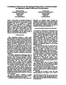
In Artificial Intelligence (AI), the classical task-planning problem1 consists in a set of operators, one initial state, and one goal state (note that there are sometimes several goals). A state is a set of propositions and their values. The instance of an operator is called an action. The world state can evolve; e.g., it evolves when an action is performed, since every performed action has usually an effect on the current world state. The objective is to select and organize actions in time that will allow one to attain the goal state by starting from the initial state. Actions can be performed only if some preconditions hold; e.g., an operation can be executed if and only if the resource it requires is in a given state. It is a complex problem to solve because it is highly combinatorial: a large number of possible actions to choose from and a huge number of conflicts that appear between actions. This problem may be much more difficult to solve if we want to optimize a criterion such as minimizing the number of actions to perform. There are some limitations to classical task planning since there is often no representation of time or resource usage. For more details, please refer to Weld, who published a survey of task planning [175]. Also, a book dedicated to automated task planning appeared recently [75]. Figure 1.1 shows a toy example of a classic planning problem in the blocks world; on the left-hand side is the initial state and on the right-hand side is the goal state. In the initial state, the two blocks are placed on a table (C and B) and block A is piled up on block B; we have to move them one after the other in such a way as to reach the goal state (A on the table, C on A, and B on C). We assume there is only one hand to move blocks and this hand can only hold one block at a time. In addition, there are some rules, called preconditions, that have to be verified to change the current world state; e.g., we cannot move a block X on Y if there is another block piled up on X or on Y . The operator in this planning problem can be expressed as follows in the STRIPS language [65]: Move(?X, ?Z, ?Y): Preconditions: Free(?Y), Free(?X), On(?X, ?Z) Effects: On(?X, ?Y), ¬ Free(?Y), Free(?Z) Operator Move requires three parameters: ?X represents the block we want to move, ?Y represents the block/table on which we want to place ?X, and ?Z represents the block/table on which ?X is placed before moving it. A solution of a planning problem is a plan; i.e., a solution is a set of actions that are partially or fully ordered. In other words, we have to find a path through the state space to go from the initial state to the goal state. A solution of the blocks world problem above is a set of three totally ordered actions: place A on the table, pile up C on A, and pile up B on C. In the STRIPS language, the solution is expressed as follows: Move(A, B, table), Move(C, table, A), Move(B, table, C). Classical task planning assumes there is no uncertainty; e.g., the effects of actions are known. This implies that outputs and inputs of the execution system are independent, this is called an open-loop execution.

1

Task planning is different from production planning since operations to execute are known in production planning and production planning focuses on the question of when to produce goods and what resources to use given production orders and due dates.

1.2. DETERMINISTIC DOMAINS

7

11111 00000 00 11 00 11 00000 11111 00000 11111 00 11 00 B 11 00000 11111 00 11 00 11 00 11 00000 11111 00 11 00000 11111 00 11 00 11 00 11 00 A 11 C 11 00 00000 11111 00 11 00 11 00 11 00000 11111 00 11 00 11 00 11 00000 11111 00 11 00 11 000000000000000000000000000000000000000000000 111111111111111111111111111111111111111111111 0000 1111 00 11 00 11 00 11 000000000000000000000000000000000000000000000 111111111111111111111111111111111111111111111 0000 1111 B C A 00 11 00 11 00 11 000000000000000000000000000000000000000000000 111111111111111111111111111111111111111111111 0000 1111 00 11 00 11 00 11 000000000000000000000000000000000000000000000 111111111111111111111111111111111111111111111 0000 1111 000000000000000000000000000000000000000000000 111111111111111111111111111111111111111111111 0000 1111 0000 1111 Free(A)

Free(B)

Free(C)

¬Free(C)

¬Free(B)

¬Free(A)

On(A, B)

On(B, C) On(C, A)

Figure 1.1: A toy example of a task-planning problem.

1.2.2

Scheduling

A classical scheduling problem comprises a set of operations and a set of resources. Each operation has a processing time and each resource has a limited capacity. The objective is to assign resources and times to operations given temporal and resource constraints; e.g., an operation cannot start before the end of another operation. The difference between task planning and scheduling is that we know what operations to perform when scheduling. In general, scheduling problems are optimization problems and typical optimization criteria are makespan, tardiness, number of tardy operations, and allocation costs. There are different structures for classifying scheduling problems; the main ones are open shop, job shop, and flow shop in manufacturing. Open-, job-, and flow-shop scheduling problems are composed of jobs, a job is a set of operations to execute, and the number of operations per job is constant. Each operation requires only one unary resource and the operations of a job require different unary resources. For open-shop scheduling problems there is no precedence constraint between the operations of a job. For job-shop scheduling problems each job is a different sequence of operations while for flow-shop scheduling problems each job defines the same sequence of operations. In project scheduling, there are all the variants of the resource-constrained project scheduling problem (RCPSP). An RCPSP is composed of a set of operations, a set of precedence constraints, a set of discrete resources (a resource may have a capacity greater than one), and a set of resource constraints. The structure of a scheduling problem depends on its temporal constraints, the number and types of resources, and how resources are allocated [109]. For a more detailed description of scheduling the reader can refer to Pinedo [125].

8


Figure 1.2 represents a small job-shop scheduling problem with three jobs. Operations are not preemptive; i.e., they cannot be interrupted once they have started to execute. Allocations have already been done and each resource; e.g., a workshop machine, can only perform one operation at a time. We assume we want to minimize the makespan of the solution, where the makespan is the duration between the start time of the first operation and the end time of the last operation of the schedule. The optimal solution of this problem is represented on Figure 1.3.

Job 1

Job 2

Job 3

000000000000000 111111111111111 000000000000000 111111111111111 11111111111 00000000000 00000000000 11111111111 000000000000000 111111111111111 Resource 1 Resource 2 Resource 3 000000000000000 111111111111111 00000000000 11111111111 000000000000000 111111111111111 00000000000 11111111111 Duration 33 Duration 46 Duration 26 00000000000 11111111111 0000000 1111111 0000000 1111111 0000000000000000000000 1111111111111111111111 0000000 1111111 0000000000000000000000 1111111111111111111111 Res. 2 Resource 1 Resource 3 0000000 1111111 0000000000000000000000 1111111111111111111111 0000000 1111111 0000000000000000000000 1111111111111111111111 Dur. 20 Duration 68 Duration 54 0000000000000000000000 1111111111111111111111 000000000 111111111 00000000000000000 11111111111111111 000000000 111111111 00000000000000000 11111111111111111 000000000 111111111 Resource 3 Resource 1 Resource 2 00000000000000000 11111111111111111 000000000 111111111 00000000000000000 11111111111111111 000000000 111111111 Duration 28 Duration 52 00000000000000000 Duration 26 11111111111111111

Figure 1.2: A toy example of a job-shop scheduling problem.

11111111111 00000000000 0000000000000000000000 1111111111111111111111 00000000000000000 11111111111111111 00000000000 11111111111 0000000000000000000000 1111111111111111111111 00000000000000000 11111111111111111 Resource 1 Resource 1 Resource 1 00000000000 11111111111 0000000000000000000000 1111111111111111111111 00000000000000000 11111111111111111 00000000000 11111111111 0000000000000000000000 1111111111111111111111 00000000000000000 11111111111111111 Duration 33 Duration 68 Duration 52 00000000000 11111111111 0000000000000000000000 1111111111111111111111 00000000000000000 11111111111111111 0000000 1111111 000000000000000 111111111111111 000000000 111111111 0000000 1111111 000000000000000 111111111111111 000000000 111111111 0000000 1111111 000000000000000 111111111111111 000000000 111111111 Res. 2 Resource 2 Resource 2 0000000 1111111 000000000000000 111111111111111 000000000 111111111 0000000 1111111 000000000000000 111111111111111 000000000 111111111 Dur. 20 Duration 46 Duration 26 Resource 3 Duration 28

Resource 3 Duration 26

Resource 3 Duration 54

makespan 179

Figure 1.3: A toy example of an optimal job-shop scheduling solution.

1.2.3

Bridging the Gap Between Task Planning and Scheduling

Many real-life problems involve both task planning and scheduling because they contain resource requirements, as well as causal and temporal relationships. In this sense, a classical planning problem is a relaxed real-world problem because it does not take into account resources and time. A scheduling problem is an overconstrained real-life problem

1.2. DETERMINISTIC DOMAINS

9

because all operations are known before scheduling and we cannot change them; no causal reasoning is done and scheduling can be seen as a sub-part of task planning that is usually not taken into account by task planning. Task planning and scheduling are complementary because each of them considers different aspects of a real-life combinatorial problem. Smith, Frank, and Jónsson demonstrated how many difficult practical problems lie somewhere between task planning and scheduling, and that neither area has the right set of tools for solving these problems [149]. Temporal planning permits one to represent time explicitly and to take a step towards scheduling. Actions have start and end times and there are delays between actions. An effect may begin at any time before or after the end of an action. Events occurring at known times can be taken into account. Planning with resources is being developed and allows to bridge the gap between planning and scheduling by taking into account resource requirements [96, 92]. Laborie worked on integrating both plan generation and resource management in a planning system [95]. At NASA Ames, a system that is based on a framework aiming at unifying planning and scheduling was developed [114]. Some researchers are working on extended scheduling problems by considering there are alternative process plans for example. A process plan is a subset of operations that are totally ordered. A subset of operations to schedule have to be chosen [90, 19]. Both classical task planning and scheduling are limited because they assume the environment is deterministic. In task planning, actions are deterministic; i.e., we know the effects that are produced when actions are performed. In scheduling, operation durations are precisely known and resources do not break down. Section 1.3 focuses on non-deterministic task planning and scheduling.

1.2.4

Models

In this section, we present some models that are used to represent static task planning and scheduling problems when execution is assumed to be deterministic. Each model is associated with a set of search algorithms to solve instances of these problems. Constraint-Satisfaction Problem A classical Constraint-Satisfaction Problem is a tuple hV, D, Ci, where V is a finite set of variables, D is the set of corresponding domains, and C = c1 , . . . , cm is a finite set of constraints. A constraint is a logical and/or mathematical relationship in which at least one variable is expressed. A solution is a complete consistent value assignment that is such that the assignment of values for the variables in V satisfies all the constraints in C. For rigorous definitions of the basic concepts, we refer the reader to Dechter [48] and Tsang [159]. Although its definition does not require it, the CSP as defined above is classically formulated for variables with discrete domains, typically a finite set of symbols or an integer interval. The CSP has also been formulated for variables with continuous domains, typically a real interval [104], when it is called a numerical CSP. Propagation algorithms, also called filtering algorithms, are used to remove values from variable domains and determine if the CSP is not consistent; i.e., a CSP is not consistent if a variable domain becomes empty after propagation. There can be different algorithms

10


with different complexities and different inference powers for a given constraint; e.g., the alldiff constraint can be implemented in different ways [131]. Propagation is initially done before starting search and then it might be incrementally done during search; i.e., whenever a variable domain is changed, a propagation is done to update variable domains with respect to constraints. A scheduling problem can be represented by a constraint network such that operation start times, operation durations, operation end times, resource capacities, and optimization criteria are variables. There are particular propagation algorithms such as temporal propagation for temporal constraints, timetables [100], edge-finder [119, 18], the balance constraint for resource capacity constraints [96], etc. A temporal task-planning problem can also be represented by a constraint network. Constraint-Based Interval (CBI) planning makes use of an underlying constraint network to keep track of the actions and the constraints in a plan [64]. For each interval in the plan, two variables are introduced into the constraint network, corresponding to the beginning and ending points of the interval. Constraints on the intervals then translate into simple equality and inequality constraints between end points. Interval durations translate into constraints in the distances between start and end points. Inference and consistency checking in the temporal network can often be accomplished using fast variations of arcconsistency, such as Simple Temporal Propagation [51]. Vidal and Geffner have recently proposed constraint propagation rules for solving canonical task-planning problems [168]. Canonical task planning is halfway between full temporal task planning and scheduling: while in scheduling, typically every action (operation) is done exactly once, in canonical task planning, it is done at most once, in full temporal task planning, it may be done an arbitrary number of times. Laborie has developed filtering algorithms for making search of minimal critical sets more efficient when planning or scheduling with resources [95, 97]. Mathematical Programming Mathematical Programming is an alternative to CSP to model and solve optimization problems when all constraints can be expressed by linear relationships. There are mainly two ways of modeling such a problem: Mixed Integer Program (MIP) or Linear Program (LP). In a MIP some variables are integers whereas there are only real variables in an LP. In general, there are more variables in a mathematical program than in a CSP but their domains are smaller. An LP is solved by the simplex method. The simplex method is very easy to use and can find optimal solutions. Branch-and-cut can efficiently solve a MIP whose continuous relaxation is a good approximation of the convex hull of integer solutions and/or around the optimal solution, or for which this relaxation can be reinforced by adding cuts. The continuous relaxation consists in removing integrality constraints and cuts are linear relationships. Lagrange multipliers, duality, and convexity can also be used to solve these programs. Compared to the CSP approach it is less easy to formalize a mathematical program and obtain a model that can be efficiently solved without exponentially increasing the number of integer variables or the number of constraints. In addition, even if some non-linear expressions can be linearized, for example the disjunctions, or the logical constraints more generally, their formulations often result in weak linear relaxations and thus in an inefficient solving. Queyranne and Schulz propose a review of some mixed integer programs with a polyhedral study [130]. For a recent

1.3. NON-DETERMINISTIC DOMAINS

11

state-of-the-art review in integer programming the reader can refer to Wolsey [178]. Several planners have been constructed that attempt to check the consistency of sets of metric constraints even before all variables are known. In general, this can involve arbitrarily difficult mathematical reasoning, so these systems typically limit their analysis to the subset of metric constraints consisting of linear equalities and inequalities. Several recent planners have used LP techniques to manage these constraints [123, 124, 157, 177]. The operations research community has been interested in solving scheduling problems by using MIP since its beginnings. In particular, some works have been done on the Resource-Constrained Project Scheduling Problem [11, 17, 66, 121, 156, 154]. In this problem, resource constraints are hard to model with linear inequalities because it is necessary to keep track of the set of operations during execution at any time. Most researchers who use MIP for modeling RCPSPs work around this problem by discretizing time, but many additional variables have to be used depending on time horizon.

1.2.5

Optimization

The solutions are not equal in every combinatorial problem. In scheduling, for instance, the user might deem schedules with shorter makespans to be preferable to those with longer makespans. Indeed, optimization is a discrimination between solutions by nature. In a constraint optimization problem (COP), solutions are ordered partially or totally according to optimization criteria [108]. An optimization criterion is an arithmetic expression over a subset of variables of the problem; e.g., tardiness depends directly on when operations finish with respect to due dates but is not directly dependent on what resources are used. Without loss of generality, solutions are sought that satisfy all constraints and minimize an objective function; e.g., we want to find a schedule that does not violate precedence and resource constraints and minimizes makespan. When using a constraintbased approach branch-and-bound can be applied to make search more efficient; e.g., a first solution is found heuristically and gives a first value of the objective function, then the problem is incrementally strengthened by posting an additional constraint bound by the best optimization value. When using a linear program to model an optimization problem with linear constraints, the simplex or interior point methods can be used to find the optimal solution if one exists.

1.3

Non-deterministic Domains

In this section, we review the literature about task planning and scheduling when we assume solutions are executed in a non-deterministic environment because unexpected events occur during execution; e.g., new goals to attain and/or new operations to perform. In some cases, we do not know precisely when some expected events occur; e.g., resource breakdown end times. In other words, the environment is imprecisely and/or partially known and its evolution is described by distributions.

1.3.1

Uncertainty Sources

Uncertainty is a general term but we can distinguish uncertainty from imprecision. An uncertain event means that we do not know if this event will occur or not whereas an

12


imprecise event means that we do not exactly know when this event is going to occur but we know for sure it is going to occur. A risk can be associated with the occurrence of an event and means the occurrence of the event impacts the solution quality. Given the occurrence of an event we are given a set of decisions to make. Each decision has a consequence. Decision theory is a research domain in which the desirability of a decision is quantified by associating a utility (or desirability) measure with each outcome. In the rest of this dissertation we shall not be concerned with risk. In this section, we list a number of uncertainty sources in task planning and scheduling without being exhaustive. In task planning, we may have to address the following problems: • some actions have imprecise effects; e.g., after having moved, the position of a robot is not precisely known; • world states are partially observable or not observable; e.g., the position of the robot is unknown because it is not equipped with sensors; • world states are uncertain independently of actions and need information gathering; e.g., a robot can reach an area by taking one of two alternative paths depending on ground composition, that is to say, the robot has to analyze a ground sample before moving; • new subgoals are added during execution. In scheduling, we may have to deal with the following problems: • some operation processing times/durations or some earliest operation start times are not precisely known a priori ; • some resource capacities or states are imprecise a priori ; e.g., the mean time between failures of a resource can be used, we do not the exact start time of a breakdown; • some resource quantities required by some operations are imprecise and/or uncertain (no resource may be required) a priori ; e.g., we do not know precisely how many workers are needed to lay the foundations of a dam because of uncertain/partial knowledge of the geological conditions before starting to work; • uncertain and/or imprecise production orders; • new operations to be scheduled and executed may only be known during execution; e.g., we have to inject some cement into the foundations because we observe they are not enough strong via specific sensors.

1.3.2

Definitions

In this section, we give some general definitions for a better understanding of the literature. The first three definitions explain some characteristics of a problem to solve such that its solution will be executed. The problem is composed of variables, such as operation durations, operation start times, or the state of a resource.


13

Definition 1.3.1 (effectiveness). An effective plan/schedule is a plan/schedule obtained after execution. An effective plan/schedule is fully set; i.e., all variables have been instantiated. After a variable is effectively instantiated, we can no longer change it. Definition 1.3.2 (event). An event is a piece of information about the world state. For example, the end time of an operation with an imprecise processing time is an event since we do not know precisely when this operation ends before observing it is finished. In other words, we do not know its effective end time date before it occurs. A dynamic problem is a problem that changes during execution, whereas a static problem does not change during execution. For example a scheduling problem is dynamic because operations are added or removed during execution, distributions associated with its random variables are changed during execution, etc. Notice that a static problem can be defined by imprecise data. For example a scheduling problem with breakable resources can be considered as a dynamic problem if the exact number of resource breakdowns is not known before execution. However, a scheduling problem with imprecise processing times is a static problem since we know the set of events in advance; i.e., we know the set of operation start and end times in advance. A deterministic problem is a static problem by nature since all events are known in advance but a non-deterministic problem; i.e., a problem with random variables can be either static or dynamic. The following definitions concern the generation process that is the procedure used to find a solution of a problem. Definition 1.3.3 (predictive decision-making process). Predictive planning/scheduling consists in making all decisions before execution starts. In the literature, some authors use the term baseline schedule instead of predictive schedule. Definition 1.3.4 (reactive decision-making process). Reactive planning/scheduling consists in making all decisions as late as possible; i.e., decisions are taken and executed without anticipation during execution. Predictive and reactive planning/scheduling are two extremes because in the former all decisions are made before execution with anticipation and in the latter no decision is made in advance. Definition 1.3.5 (off-line reasoning). Off-line reasoning consists in taking decisions before execution starts. When reasoning off line a predictive schedule/plan is typically generated off line and passed on to the execution manager. This reasoning is usually static; i.e., the predictive schedule/plan is completely generated and all decisions are taken at the same time. Such a reasoning is deliberative; i.e., we take decisions in advance of their executions and we have time to reason.

14


Definition 1.3.6 (on-line reasoning). On-line reasoning is concurrent with the physical process execution. On-line reasoning is dynamic by nature because the generation of a schedule/plan is incremental ; i.e., the schedule/plan is completed as long as execution goes on. This reasoning usually needs to meet real-time requirements; i.e., decisions have to be made given a time limit. Such a reasoning can be deliberative and/or reactive to events. It is also possible to change decisions during execution. Table 1.1 summarizes the characteristics of the generation and execution processes under uncertainty and/or change. When a solution is executed, some elements of its execution environment may change; e.g., the state of a resource changes. In general, there are real-time requirements when executing a solution; i.e., if some basic decisions have still to be made the time for computation is limited; e.g., operation start times have to be quickly decided. Execution decisions are decisions to adapt the flexible solution with respect to what happens during execution. The decision-making system might be able to react in response to occurring events; i.e., it can make execution decisions when some events occur. For example, when the state of a resource changes, we may have to decide what alternative operations to execute. The generation of a solution can be made off and/or on line. When a solution is generated off line we usually have time to make decisions whereas we have a limited time for making decisions during execution due to the dynamics of the underlying physical system and its execution environment. Generation decisions are decisions made to anticipate what is going to happen during execution. Sometimes the system must be able to change decisions on line when the solution is no longer executable; e.g., a resource breaks down and we have to reallocate some operations that have to be executed in the near future.

Dynamic=changes over time: states. . . Real time=timebounded computation Reactive=in response to events

Execution Process: solution being executed on line Yes Yes, but only basic decision-making Might be

Generation Off-line On-line scheduling/ scheduling/ planning planning Usually not Yes No

Yes

No

Might be

Table 1.1: Off-line/On-line reasoning. In the ideal world, there is no unexpected event that can occur and affect the schedule/plan quality or make the schedule/plan unexecutable during execution, so the predictive plan/schedule is generated off line and then executed. Figure 1.4 represents the generation-execution loop in the ideal world. A plan/schedule is generated off line and sent to the execution controller. The latter drives the underlying physical system by sending orders (actions) to actuators. The sensors of the physical system send information (events) to the execution controller that updates the plan/schedule accordingly; i.e., it indicates what events have been executed and updates clock. The execution controller


15

plays the role of an interface between the solution generator and the physical system. Note however that in the case of the ideal world we do not need to observe events since there is no unexpected event and the occurrences of events are precisely known.

Planning/ Scheduling

off line on line

Plan/ Schedule update Events Execution controlling Actions

solution execution

real world

Figure 1.4: Generation and execution in the ideal world. However, the predictive schedule/plan will not always fit the situation at hand because there are uncertainty and change; i.e., data is imprecise and/or uncertain. In such a situation, we have to decide what to do to cope with uncertainty and change: we could adapt the schedule/plan on line, we could make the initial schedule/plan less sensitive to execution environment, and/or we could find a compromise between both options; Sections 1.3.5 and 1.3.6 present some techniques to handle uncertainty and change. The next section is dedicated to reviewing uncertainty sources in task planning and scheduling.

1.3.3

Uncertainty Models

A number of different models have been proposed and used to represent uncertainty in scheduling and task planning. In this section, we present these uncertainty models and give their main properties. Moreover, we discuss Bayesian approach since it is a promising way for dealing with uncertainty in scheduling and planning.

16


Probability Theory The probability theory is based on the notion of sets; it uses unions and intersections of sets. In the probability theory a random variable X can be instantiated to value v belonging to a discrete or continuous domain D; i.e., it is a probability distribution Pr(X = v). The formal definition is the following: ∀v ∈ D, 0 ≤ Pr(X = v) ≤ 1 and if we comP pletely know the probability distribution: v∈D Pr(X = v) = 1. It is possible to express dependence between variables. A conditional probability such as the occurrence of event A knowing the occurrence of event B is expressed as follows: Pr(A|B) =

Pr(A, B) , Pr(B)

where Pr(A, B) is the probability that both A and B occur at the same time and is called the joint probability. This is then possible to compute the marginal probability of A: P Pr(A) = v∈D (Pr(A|X = v) × Pr(X = v)). If A and B are independent events then: Pr(A, B) = Pr(A) × Pr(B). Probabilities can be used to model imprecise operation processing times [21] or action effects in task planning [32] but they require statistical data that do not systematically exist. In addition, probabilities are easy to interpret but cannot represent full or partial ignorance. Bayesian Networks Bayesian networks are acyclic directed graphs [122]. Each node is associated with a finite domain variable, each variable domain is associated with a probability distribution, and each arc represents a causal relation between two variables. Each pair of dependent variables is associated with a table of conditional probabilities. For example if the duration of an operation depends on the outside temperature and humidity this yields the Bayesian network of Figure 1.5a, where Figure 1.5b depicts the link matrix necessary for full characterization of the causal relation. According to this matrix we know that the probability that the operation duration is 15 minutes if the outside humidity is less than 40 per cent and the outside temperature is less than 20◦ Celsius equals 0.1. A Bayesian network contains the information needed to answer all probabilistic queries. A Bayesian network can be used for induction, deduction, or abduction. Induction consists in determining rules by learning from cases, just like neural nets. Deduction is a logic procedure in which we reason with rules and input facts to determine output facts. Abduction is a way of reasoning such that output facts are symptoms that are observed whereas decisions must be taken as which input facts produced the observed symptoms. A Bayesian network is a static representation (no anteriority); it can not represent time but is able to model incomplete knowledge. Bayesian networks have some limitations. Inference in a multi-connected Bayesian network is NP-hard. Variables are discrete, and the number of arcs is limited for performance reasons. In addition, Bayesian inference can only be done with a complete probabilistic model. However, when dealing with discrete probability distributions associated with some input facts it is possible to compute approximate probability distributions of output facts by using Monte-Carlo simulation. The only issue when generating a realization is to pick up first the random values of the independent variables. Bayesian networks have the


17

operation duration

outside temperature

outside humidity

operation duration

(a)

outside humidity outside temperature < 40% < 20◦ Celsius between 40% and 60% < 20◦ Celsius > 60% < 20◦ Celsius < 40% between 20◦ and 30◦ Celsius between 40% and 60% between 20◦ and 30◦ Celsius > 60% between 20◦ and 30◦ Celsius < 40% > 30◦ Celsius between 40% and 60% > 30◦ Celsius > 60% > 30◦ Celsius

15 minutes 25 minutes

0.1

0.9

0.2

0.8

0.3

0.7

0.4

0.6

0.35

0.65

0.25

0.75

0.85

0.15

0.95

0.05

0.45

0.55

(b)

Figure 1.5: (a) A Bayesian network and (b) a conditional probability matrix characterizing the causal relation.

same advantages and drawbacks as probabilities: it requires statistical data and cannot represent ignorance. Recently some work has been done to combine CSPs with Bayesian Networks [128]. Influence diagrams [86] extend Bayesian networks by adding random utility variables and non random decision variables to the usual random variables. A non random decision variable is instantiated by a decision-maker, and random utility variables are used to represent the objective (or utility) to be maximized. Dynamic Bayesian Networks [47] (DBNs) are another extension to Bayesian networks that can model dynamic stochastic processes. A DBN can model changes in a world state over time. DBNs fail to model quantitative temporal constraints between actions in a computationally tractable way and suffer from the problem of unwarranted probability drift; i.e., probabilities associated with facts depend upon how many changes in the world state have occurred since the last time probabilities were computed. Hybrid or mixed networks [49, 50] allow the deterministic part of a Bayesian network to be represented and manipulated more efficiently as constraints.

18


Theory of Fuzzy Sets and Possibility Theory Zadeh has introduced the theory of fuzzy sets that is based on the generalization of the notion of set [181]. The characteristic function of a subset A of a universal set Ω associates the value 1 to any element of Ω if this element is in A and the value 0 if this element is not in A. On the contrary, for a fuzzy subset it is possible to define intermediate membership degrees between these two extremes. More formally, a fuzzy subset is defined as follows. A fuzzy subset A of a universal set Ω is defined by a membership function µ : Ω → [0, 1]. For any element ω in Ω the value µA (ω) is interpreted as the membership degree of ω to A. The possibility theory is a convenient means to express uncertainty [182]. With this theory it is possible to explicitly take into account uncertainty associated with the occurrences of events. In such a model uncertainty associated with an event e is described by a possibility degree that e occurs and a possibility degree that the opposite event e occurs. In general, a possibility distribution over a universal set Ω (the set of possible events) is a function π : Ω → [0, 1] defined such that there exists at least one ω ∈ Ω such that π(ω) = 1. From a possibility distribution over Ω it is possible to define a possibility measure Π and a necessity measure N of a part A of Ω as follows: Π(A) = sup π(ω) and N (A) = infA (1 − π(ω)), ω∈A

ω∈CΩ

where CΩA is the complementary part of A in Ω. Notice that for any part A of Ω, the possibility measure and the necessity measure are related by the following formulas: N (A) = 1 − Π(CΩA ) and Π(A) ≥ N (A). In practice, different interpretations of these functions π can be made. • It is possible to represent an occurrence possibility with π(X = v); i.e., the possibility that variable X is instantiated with value v. • We can express similarity with π(E is cpt) that represents the degree to which element E is similar to concept cpt (represented by a function); e.g., Figure 1.6 represents a similarity function with respect to the concept “young.” • It is also possible to express preferences with π(X = v) that represents the satisfaction degree when variable X is equal to value v. With a possibility function, it is possible to represent both imprecision and uncertainty. For example we can represent the fact that we do not know precisely and with total certainty how many workpieces are produced in a workshop; we can only express a possible and imprecise number between 200 and 400, the possible fact that no workpiece are produced at all, and it is not fully possible but we may produce 600 workpieces; Figure 1.7 represents such a possibility function. Such a function can also represent the fuzzy processing time of an operation for example, see Section 1.3.6. The classical concept of set is limited for representing vague knowledge, and probability theory is not able to represent subjective uncertainty and ignorance, however, fuzzy logic and the theory of possibility overcome these difficulties. The main drawback of the fuzzy representation is the subjective way for interpreting results.


19

1

0.8

0.6

0.4

0.2

0

0

10

20

30

40

50 60 Age (years)

70

80

90

100

Figure 1.6: A possibility function of the concept “young.”

1

0.5

0

0

100

200

300 400 500 Number of produced workpieces

600

700

Figure 1.7: A possibility function for a number of produced workpieces.

20


T (room3 , moveright , t1 ) = 0.7 T (room4 , moveforward , t1 ) = 0.2

T (room4 , moveforward , t1 ) = 0.8

1111 0000 0000 1111 0000 1111 0000 1111 0000 1111 robot in room 4

robot in room 3 R(room3 ) = −4 T (room4 , moveright , t1 ) = 0.3 R(room4 ) = 3

T (room4 , moveright , t1 ) = 0.7

robot in room 6

T (room6 , moveleft, t1 ) = 0.1

robot in room 5

R(room6 ) = −1

T (room6 , moveleft, t1 ) = 0.9

T (room5, moveforward , t1 ) = 0.4

R(room5 ) = 5

T (room5, moveforward , t1 ) = 0.6

robot in room 7

R(room7 ) = 6

Figure 1.8: An illustrative example of the graphical view of an MDP. Markov Decision Processes A Markov Decision Process can be seen as a timed automaton such that each transition from one state to another state is associated with a probability of being fired. More formally an MDP can be defined as follows: an MDP has four components, S, A, R, T . S (|S| = n) is a (finite) state set. A (|A| = m) is a (finite) action set. T (s, a, t) is a transition function that depends on time t, and each T (s, a, −) is a probability distribution over S represented by a set of n × n stochastic matrices.2 R(s) is a bounded, real-valued reward function represented by an n-vector. R(s) can be generalized to include action costs: R(s, a). R(s) can be stochastic (but replaceable by expectation). MDPs can model transition and/or stochastic systems; i.e., it is possible to model how a process evolves during execution (the state of a system can change over time depending on what actions are performed) [70, 129]. MDPs are related to decision-theoretic planning [33] and used to model state-spaces in the task-planning context. General objective functions (rewards) can be expressed. Policies are general solution concepts that consist in choosing what action to perform in each visited state to maximize the total reward. MDPs provide a nice conceptual model: classical representations and solution methods 2

Note that Sabbadin [135] proposed to use possibilistic MDPs.


21

tend to rely on state-space enumeration whereas MDPs are able to easily represent this space. Figure 1.8 is a graphical view of MDP that represents the state space of a small task-planning problem in which a robot must go from room 3 to room 7. There are three operators: move right, move left, and move forward. This MDP is valid at time t1 when the robot is in room 4. In the current state, only one of two actions can be performed: move either right or forward. If action moveforward is activated, the probability that the robot does not move is equal to 0.2 and the probability that it actually goes from room 4 to room 6 equals 0.8. Each state s represents the possible position of the robot; i.e., s indicates the room it is in. The probabilities that are not represented equal zero. MDP is a model easily generalizable to countable or continuous state and action spaces. The main drawback of MDP is the need to enumerate and represent all possible states; i.e., it is time and memory consuming. Partially Observable MDPs [106] take into account the fact that each state of the dynamic process is generally indirectly observable via potentially erroneous observations. In task planning, an observation consists in general in performing an action to gather new information. Dynamic programming [23, 24] is used to solve MDPs. The main issue of MDPs is the number of states to develop; so some work has been done for finding a more compact representation; for example, Factored MDPs [34] extend MDP concepts and methods to a variable-based representation of states and decisions. Sensitivity Analysis Sensitivity analysis consists in defining how much we can perturb a problem without degrading the quality of the solution of the initial problem. In other words, sensitivity analysis, combined with parametric optimization, is a way of checking if the solution of a deterministic linear program is reliable, even if some of the parameters are not fully known but are instead replaced by estimated values. When doing a sensitivity analysis, we are interested in knowing the robustness of a solution; i.e., to what extent this solution is insensitive to changes of the initial problem with respect to its quality, in particular, what are the limits to a parameter change (or several changes) such that the solution remains optimal? However, sensitivity analysis has some limitations since it is based on deterministic models and is thus useful only as far as variation of controllable parameters is concerned [171]. Application of sensitivity analysis has been done in scheduling [78, 153]. Stochastic Programming Stochastic programming [29] is a mathematical programming paradigm, see Section 1.2.4, which explicitly incorporates uncertainty in the form of probability distributions of some parameters. There are decision variables and observations; i.e., observations are values of the random parameters. In a recourse problem, decisions alternate with observations in an m-stage process; i.e., at each stage, decisions are made, and observations are done between stages; there are initial decisions made before any observation and recourse decisions made after observations. The number of stages gives a so-called finite horizon to the process. A decision made in stage s should take into account all future realizations of the random parameters and such decision only affects the remaining decisions in stages s + 1, s + 2 . . . m. In Stochastic Programming, this concept is known as non-anticipativity.

22


The convex optimization function depends on decisions and observations. The goal is to optimize the expected value of the optimization function such that random parameters are not necessarily independent of each other; they are however independent of decisions. One approach to solving this problem is to use an expected value model that is constructed by replacing the random parameters by their expected values. Another solving process consists in generating n scenarios such that each scenario; i.e., any possible set of values for the parameters represents a deterministic mathematical program that is then solved [55]. Once the n programs have been solved, decisions that are common to the most solutions are made for solving the stochastic program. One of the issues of this approach is the number of scenarios that are necessary to solve the problem and the related efficiency issue. Extensions of the Constraint-Satisfaction Problem We review the main constraint-satisfaction problem frameworks that can deal with uncertainty and change. For a more detailed review, the reader can refer to the recent paper of Verfaillie and Jussien [162]. These frameworks are extensions of the ConstraintSatisfaction Problem framework presented in Section 1.2.4. Dynamic CSP A Dynamic Constraint-Satisfaction Problem (DCSP) consists in a series of CSPs that change permanently or intermittently over time, by loss or gain of values, variables or constraints. The objective is to find stable solutions to these problems; i.e., solutions that remain valid when changes occur. Wallace and Freuder tackled these problems [169]. The basic strategy they use is to track changes (value losses or constraint additions) in a problem and incorporate this information to guide search to stable solutions. The objective for them is to find a trade-off between solution stability and search efficiency. A probabilistic approach is used: each constraint C is associated with a value that gives the probability that C is part of the problem. Probabilities of change are not known a priori. Elkhyari et al. study scheduling problems that change during execution and use DCSPs to model and solve them [56]. In particular, they study Resource-Constrained Project Scheduling Problems. They use explanations by determining conflict sets, also known as nogoods, to solve these problems. Conditional CSP The Conditional Constraint-Satisfaction Problem [137] framework (CCSP) was first named Dynamic Constraint-Satisfaction Problem [111]. CCSPs have been studied by a number of researchers [35, 136, 152, 71, 138]. The basic objective of the CCSP framework is to model problems whose solutions do not all have the same structure; i.e., do not all involve the same set of variables and constraints. Such a situation occurs when dealing with product configuration or design problems, because the physical systems that can meet a set of user requirements do not all involve the same components. More generally, it occurs when dealing with any synthesis problem, such as design, configuration, task planning, scheduling with alternatives, etc. In a CCSP, the set of variables is divided into two parts: a subset of mandatory variables and a subset of optional ones. The set of constraints is also divided into two parts: a subset of compatibility constraints and a subset of activity constraints. Compatibility constraints are classical constraints. Activity constraints define the conditions of activation of the optional variables as functions of the


23

current assignment of other mandatory or optional variables. Constraints are activated if their respective variables are activated too. When solving a CCSP its structure (activated variables and constraints) may change because it depends on the current assignment. Thus, a CCSP can be considered as a particular case of DCSP where all the possible changes are defined by the activity constraints. Open CSP The Open Constraint-Satisfaction Problem [60] framework (OCSP) was first named Interactive Satisfaction Problem [98]. In an OCSP, the allowed values in domains, as well as the allowed tuples in relations, may not be all known when starting search for a solution. They may be acquired on line when no solution has been found with the currently known values and tuples. Such a situation occurs when the acquisition of information about domains and relations is a costly process that needs either heavy computation or requests to distant sites. An OCSP can thus be considered as a particular case of DCSP where all the possible changes result in extensions of the domains and relations. Mixed CSP The Mixed Constraint-Satisfaction Problem [63] framework (MCSP) models decision problems under uncertainty about the actual state of the real world. In an MCSP, variables are either controllable (decision variables) or uncontrollable (state variables). Decision variables are under the control of the decision agent whereas state variables are not under its control. In this framework, a basic request may be to build a decision (an assignment of the decision variables) that is consistent whatever the state of the world (the assignment of the state variables) is. An MCSP can not model problem changes but imprecision, therefore MCSP and DCSP are complementary. Probabilistic CSP The Probabilistic Constraint-Satisfaction Problem framework (PCSP) models decision problems under uncertainty about the presence of constraints [61]. In a PCSP, a probability of presence in the real world is associated with each constraint. In such a framework, a basic request may be to produce an assignment that maximizes its probability of consistency in the real world. A PCSP is a particular case of the Valued Constraint-Satisfaction Problem framework (VCSP) [144, 30]. Fuzzy CSP The Fuzzy Constraint-Satisfaction Problem framework (FCSP) models decision problems where possibility distributions are associated with variable domains [134]. In such a framework, we are interested in finding a solution that satisfies constraints and maximizes the satisfaction degree whatever the effective instantiations of variables turn out to be. The satisfaction degree of a solution is the combination of the possibility degrees corresponding to the assigned values. This framework is subsumed by the semiring-based CSP framework [30]. Stochastic CSP The Stochastic Constraint-Satisfaction Problem [172] framework (SCSP) models decision problems under uncertainty about the actual state of the real world, the same way as the MCSP framework. The SCSP framework is inspired by the Stochastic Satisfiability Problem framework (SSAT) [105]. As in an MCSP, variables are, in an SCSP, either controllable (decision variables) or uncontrollable (state variables). The

24


main difference between an MCSP and an SCSP is that decision variables have not necessarily to be instantiated before state variables in an SCSP. In such a framework, a basic request may be, as in a PCSP, to build a decision (an assignment of the decision variables) that maximizes its probability of consistency in the real world. A recent proposal, the Scenario-based Constraint-Satisfaction Problem [107] framework, is an extension of SCSP along a number of dimensions: multiple chance constraints and new objectives. It is inspired by Stochastic Programming, see Section 1.3.3. In this framework, there are two kinds of constraints: hard constraints that must always be satisfied and chance constraints which may only be satisfied in some of the possible worlds. Each chance constraint has a threshold, θ and the constraint must be satisfied in at least a fraction θ of the worlds. Stochastic constraint programs are closely related to MDPs 1.3.3. Stochastic constraint programs can, however, model problems which lack the Markov property that the next state and reward depend only on the previous state and action taken. The current decision in a stochastic constraint program will often depend on all earlier decisions. To model this as an MDP, we would need an exponential number of states.

1.3.4

Temporal Extensions of CSPs

In this section, we describe some extensions of the CSP framework that can deal with time. Therefore, these frameworks are particularly suited to temporal task planning, scheduling, and other temporal application domains. Temporal Conditional CSPs Conditional CSPs have been adapted to temporal problems to be able to represent alternatives. An alternative is a subset of temporal constraints. By nature, each alternative belongs to a set whose elements are mutually exclusive. Tsamardinos, Vidal, and Pollack [158] have proposed a new constraint-based formalism with temporal constraints. In this paper, they present a procedure that is able to check whether such a constraint network is consistent whatever alternatives are chosen. Temporal CSPs with Uncertainty The Temporal CSP with Uncertainty framework is directly inspired by MCSPs and applied in the temporal context. A usual strategy to deal with uncertainty, referred to as least commitment strategy, consists in deciding about some crucial choices (for example the selection and sequencing of operations) and letting another process (for example execution control) make the remaining decisions (for example the start times of the selected and sequenced operations) according to information coming from actual execution. In such a situation, the problem is to be sure that the remaining decisions will be consistent whatever the actual situation. In the Simple Temporal Problem with Uncertainty framework [166], an extension of the Simple Temporal Problem framework [51] to deal with uncertain durations, notions of controllability [166, 112], sequentiability [164, 87], dispatchability [170] and associated algorithms have been defined to offer such a guarantee. Temporal constraint-based models are often used, based on intervals or time points. For example, a team of robots that have to move containers from one place to another one [167]. The problem consists in allocating tasks (actions) to robots in such a way that


25

we minimize makespan. Each robot can move in different directions, pick up a container, or put down a container. In addition, there are imprecise time windows for pickup and put-down actions. This is a typical scheduling problem with uncertainty and allocation. Execution and decision-making are interleaved because decisions are easy to take in the short term, but in a longer term uncertainty increases and makes the choice less obvious, so the solution is to wait until execution gives occurrence times of events that decrease uncertainty and make the next choice possible.

Temporal CSPs with Uncertainty and Preferences Rossi, Venable, and Yorke-Smith have recently proposed a framework that integrates both Simple Temporal Problems with Uncertainty (STPU) and Simple Temporal Problems with Preferences (STPP) [132]. The notions of controllability are extended to STPPU, and methods are described to determine whether these properties hold.

1.3.5

Task Planning under Uncertainty

In this section, we review the main task-planning approaches for handling uncertainty. When planning tasks in a non-deterministic environment, effects of some actions are not deterministic. This makes us do observations during execution to get information about the actual state in order to guide the choice of the next action to execute. This means outputs of the execution system have consequences that become inputs of the execution system, this is called a closed-loop execution.

Probabilistic Planning In probabilistic planning, we assume the initial state is not known completely, effects of actions are non-deterministic, and a probability distribution over states is known and updated each time an action is performed. Adopting a probabilistic model complicates the search for a solution plan. Instead of terminating when the standard planner builds a plan that provably achieves the goal, the probabilistic planner terminates when it builds a plan that is sufficiently likely to succeed; i.e., its algorithm produces a plan such that the probability of the plan achieving the goal exceeds a user-supplied probability threshold, if such a plan exists. Kushmerick et al. developed BURIDAN, a probabilistic planner [93]. Partially Observable MDPs [32] can be used to tackle such problems, see Section 1.3.3.

Possibilistic Planning Possibilistic planning is similar to probabilistic planning except that we assume the knowledge of a possibility distribution over states instead of a probability distribution. Da Costa Pereira developed a possibilistic planner, POSPLAN [41]. Contrary to most planning systems that define actions with preconditions, POSPLAN relies on a formalism where actions are modeled by the exhaustive set of possible conditions.

26


Conformant Planning Conformant planning consists in developing non-conditional plans that do not rely on sensory information, but still succeed no matter which of the allowed states the world is actually in; i.e., we assume there is no possible observation of the states. In such a case, we need a plan that will reach the goal whatever the actual situation is. Smith and Weld developed and tested a conformant planner, CGP [150]. This planner generates sound (non-contingent) plans when faced with uncertainty in the initial conditions and in the outcome of actions. The basic idea is to develop separate plan graphs; i.e., there is one plan graph for each possible world. This requires some subtle changes to both the graph expansion and solution extraction phases of Graphplan [31]. In particular, the solution extraction phase must consider the unexpected side effects of actions in other possible worlds, and must confront any undesirable effects, such as induced mutually exclusive (mutex) relationships. Under the semantics of BURIDAN [93], it is assumed that it is not possible to observe the effects of actions, and the agent executes the same sequence of actions regardless of the effects of previous actions. Conditional Planning Conditional planning consists in defining alternatives; e.g., subsets of actions that are partially ordered. State-based planning is an extreme case where all alternatives are developed such as an MDP, see Section 1.3.3. The problem consists in generating a contingent plan that is executable [126]. The plan comprises a set of alternatives but only a subset of alternatives will effectively be executed with respect to observations made during execution. This approach can also be applied to scheduling. Sensory Graphplan (SGP) is an extension of CGP developed by Weld, Anderson, and Smith [176]. A plan graph is developed for each possible initial state. Observation actions are introduced between plan graphs. As soon as an observation action can be performed, propositions are added to distinguish one graph from another one. SGP uses CSP techniques to visit efficiently the nodes of plan graphs. Continuous Planning Continuous planning consists in updating/extending/changing the current plan by adding new tasks during execution. Paolucci et al. proposed a multi-agent system [120] that plans continuously. Their agents behave deliberatively; i.e., these agents cooperate during execution because each of them knows only partially the world state and produces local plans. The execution world is dynamic since new sub-goals are known on line and plans have to be completed accordingly. When continuously planning replanning can be used to change decisions when the current plan is no longer executable; i.e., it cannot reach the goal state any more. Sapena and Onaindia presented SimPlanner, an integrated planning and executionmonitoring system [143]. SimPlanner is a planning simulator specially designed for replanning in STRIPS-like domains. A state of the world is expressed as a set of literals. The proposed algorithm repairs the plan as a whole and finds the optimal solution; i.e., the plan with the minimal number of actions necessary to reach the current goal. This


27

modification tries to retain as much of the original plan as possible without compromising the optimal solution when some literal changes. Literals can be removed from or added in the world during execution via a graphical user interface. A number of different small planning problems were experimented, such as mobile robots bringing letters from offices to other offices. Chien et al., in a space exploration context [40], applied continuous planning. Planning is done on board to speed the replanning process when a failure occurs or a science opportunity is observed. Science requests are up-linked and results are down-linked. At each time, the system updates the current plan, goals, state, and next predicted states by using a telescoping-time horizon approach. When a plan failure happens, an iterative repair procedure, which is a greedy search algorithm, is applied in the short-term horizon to change allocations, move, renew, or remove actions. An extension of the system was proposed by Estlin et al. to manage a team of robots [59]. This is a centralized-distributed approach. Goals are dispatched and an abstract plan is maintained in a centralized way. Rovers share a unary resource, a lander, that gathers data and up-links them to an orbiter. However, more detailed planning and replanning are distributed; i.e., each rover continuously updates its own plan. The main advantage is the redundancy of the system because when a rover fails to achieve goals they might be reassigned to another rover. Washington et al. used a continuous planning technique for controlling a planetary rover with limited capacity resources and uncertainty [173]. A nominal flexible and conditional plan, which contains contingent plans that are chosen synchronously after observation and alternate plans that are asynchronously triggered when some conditions become true, is up-linked. During execution, an executive is in charge of managing resources and identifying conflicts. If a conflict is detected, various recoveries are possible; i.e., a contingent plan matches the situation, an alternate plan is started possibly with anticipation, actions are performed to put the system back in a stable state, and replanning is done, or the conflict is ignored because it is too far in the future. Upon failure, short-term recovery plans can be computed by the state identification module and the resource manager provides on-board rescheduling capabilities; e.g., reallocation if a resource is broken down. Lemai and Ingrand proposed a general control architecture that is able to interleave planning and execution of an autonomous system in an uncertain world [101, 102]. This approach integrates deliberative planning, plan repair, and execution control. Partially ordered and partially instantiated plans are generated and allow the insertion of new actions and/or new goals during execution. The generated plans are based on Simple Temporal Networks, see Section 1.3.4.

1.3.6

Scheduling under Uncertainty

In this section, we present some existing approaches to model and solve scheduling problems under uncertainty. There exist recent surveys dedicated to this issue [83, 43, 27]. Dispatching Rules One of the possibilities to hedge against uncertainty and change when scheduling is to schedule operations by using priority rules; e.g., an operation is allocated to and sequenced first on a machine because its processing time is the smallest [125]. Dispatching rules can

28


be either local, when a sub-problem is considered, or global, when decisions are made after considering the whole problem. The main advantage to using priority rules is the low computational cost. Such a rule can be applied on line without violating real-time constraints. It is thus possible to build a schedule incrementally during execution in a non-deterministic, indeed chaotic environment; i.e., it is possible to make a scheduling decision at the last time after having observed unexpected events. The main drawback of dispatching rules is the suboptimal quality of the solution because of their greedy behaviors (there is no backtrack mechanism). Redundancy-based Scheduling Redundancy-based scheduling consists in generating schedules with temporal slacks; i.e., we are looking for schedules with the minimal number of critical paths. In other words, the objective is to produce fault-tolerant predictive solutions by using knowledge about uncertainty. Davenport, Gefflot, and Beck proposed a redundancy-based scheduling approach in which they add slack to critical operations; i.e., operations that are allocated with possibly breakable resources [45]. This work extended the Master’s thesis of Gao [68]. The new temporally protected problem can then be tackled with techniques usually used to solve deterministic scheduling problems; e.g., constraint propagation algorithms can be used to make tree search easier, see Section 1.2.4. More precisely, operation durations are set to be longer than the original ones to generate a predictive schedule that can face possible machine breakdowns. The operation durations used are based on breakdown statistics; e.g., the so-called mean time between failures or mean time to repair may be used. Experiments on job-shop problems show that this technique reduces significantly the gap between the predicted quality and the effective quality but it results in an increase of tardiness. However, the temporal protection given to an operation o1 , which should allow the following operation o2 allocated to the same resource to start earlier if no breakdown occurs, can be “lost” if a constraint prevents o2 from starting earlier. This observation is at the outset of two methods, time-window slack and focused time-windows slack, presented by Davenport et al. who proposed to post additional constraints such that each operation has a minimum temporal slack. Simulation results show that these two methods are able to generate schedules whose tardiness is smaller than the tardiness of the schedules determined by the temporal protection technique. It is also shown that effective quality is predicted more accurately; i.e., quality predicted a priori (before execution) is closer to the effective quality, observed a posteriori (after execution). Although this approach is not based on real theoretical foundations it is simple and pragmatic such that it can be readily applied to a real scheduling problem. Leus and Herroelen use redundancy-based techniques to minimize the expected weighted deviations of the operation start times when operation durations are imprecise [103, 84]. They tackle resource-constrained project scheduling problems. Only a subset of operation durations are random. A probabilistic model of the disruptions is used and permits them to use Monte-Carlo simulation for selecting solutions. Their study assumes a multi-project environment and thus operations cannot be started before their foreseen starting times in the predicted schedule. Some operation start times may need to be better protected than others; for instance, because of varying difficulties to release the required resources at later


29

times, or for reasons of coordination with external parties, or simply because of the value to the customer of the projected dates being met. Actual probability distributions that apply during project execution are not known beforehand, and the discrete input scenarios form the best approximation available. Leus and Herroelen introduce some redundancy by adding slack times between operations, they trade off makespan against protection of operation start times. Daniels and Carillo worked on a scheduling problem in which the goal is to find the schedule that minimizes the probability of performance less than a threshold [42]. It is a one-machine problem with uncertain operation durations. The idea is to use the uncertainty statistics; i.e., means and variances, to find such a schedule called the “β-robust schedule.” It is an NP-hard problem [69]. Solution techniques consist in a branch-and-bound where sequence is assigned chronologically, dominance rules are used and bounds are based on partial sequence. Dominance rules are heuristics. An approximation technique is used as follows: we repeatedly and reactively generate schedules by applying the Shortest Processing Time priority rule for “well-chosen” scenarios and we evaluate the probability that the tardiness of the schedule is less than T . The concept is similar to probabilistic customer service in inventory management. Probabilistic customer service allocates inventory so that there are probabilistic guarantees on achieving full customer service. For example, a 95% customer service level means that 95% of the time all customer orders will be met from the stored inventory. Redundancy-based scheduling is better than dispatching since it does not make decisions myopically. However, performances of redundancy-based scheduling rely on how much distributions are reliable. Contingent Scheduling The contingent scheduling approach consists in generating a set of predictive schedules off and/or on line such that they perform optimally when anticipated disruptions occur. In case a disruptive event occurs during execution, it is possible to switch to the optimal schedule that matches best the situation at hand. Notice that the set of predictive schedules can be explicitly enumerated. Drummond et al. proposed a contingent scheduling method, called Just-In-Case (JIC) scheduling, applied to a real-world telescope observation scheduling problem where observation durations are uncertain [53]. The solution consists in building a contingent schedule that takes into account likely failures of the telescope. The objective is to increase the percentage of the schedule that can be executed without breakage by assuming there is a scheduling algorithm for solving the deterministic problem, and probability distributions of the observation durations are known; i.e., the mean values and the standard deviations are known. The JIC scheduling proceeds as follows. Before execution we identify the most likely breakage, split the schedule accordingly, and then find a new schedule assuming the breakage. There are of course several likely breakages, so the procedure is applied several times. During execution, if there is no breakage, we keep executing the same schedule, otherwise, if the situation is covered by the contingent schedule, we switch to a new schedule. This is a successful, real-world solution. The on-line portion is trivial since we only have to switch to schedules. However, this method is applied to a one-machine scheduling

30


problem and the combinatorial complexity seems to hinder its generalization to multiple machine problems. To reduce the complexity due to explicit enumeration, other works focus on partial-order schedules, see the next section. Contingent scheduling is more optimal than redundancy-based scheduling since it generates a family of schedules that better fit to the actual situation. However, the generation and the storage of solutions are costly and increase with the size of the faced problem. Partial-Order Scheduling A number of researchers have used partial-order schedules (POSs) to handle uncertainty. Some people use the concept of “group of operations;” i.e., a group of operations is a subset of operations allocated to the same resource that can be totally permuted without violating problem requirements [26, 15, 58, 16]. This approach assumes unary resources. The main idea is to build a POS before execution such that a sequence of groups is determined for each resource. One of the advantages of such an approach is the possibility to quickly compute the worst performances of the POS with respect to optimization criteria. It is also possible to reduce the number of possible permutations in a group to guarantee minimal performances [12]. The POS is then used on line as follows: ordering of the operations of a same group are made either manually by a decision-maker based on performance indicators, or automatically by applying dispatching rules, see Section 1.3.6. More recently, La proposed another off-line generation method based on partial-order scheduling [94]. He uses the notion of interval structure, and of dominant or sufficient conditions regarding the admissibility or optimality of scheduling solutions. These partial orders allow the determination of the best and the worst performances of the characterized solution set, in terms of lateness, in polynomial time. La tackles a one-machine problem and demonstrates that it is possible to find a dominant set of solutions whose performances are insensitive to a number of scenarios if effective release dates and/or operation processing times and/or due dates are imprecise; i.e., possible realizations are modeled with intervals, and for each operation the two intervals associated with release and due dates have not to overlap. Policella et al. also considered the problem of generating POSs for problems with discrete resources [127]. They actually tackle resource-constrained project scheduling problems with using filtering algorithms and propose two orthogonal procedures for constructing a POS. The first, which is called the resource envelope based approach, uses computed bounds on cumulative resource usage; i.e., a resource envelope, to identify potential resource conflicts, and progressively reduces the total set of temporally feasible solutions into a smaller set of resource feasible solutions by resolving detected conflicts.3 The second, referred to as the earliest start time approach, instead uses conflict analysis of a specific; i.e., earliest start time, solution to generate an initial fixed-time schedule, and then expands this solution to a set of resource feasible solutions in a post-processing step. As might be expected, the second approach, by virtue of its more focused analysis, is found to be a more efficient POS generator based on experimental results. Wu et al. proposed another way of producing partial-order schedules [179]. They identify a critical subset of decisions that, to a large extent, dictate global schedule performance. These critical decisions are made off line and the rest of the decisions are done during execution. Before execution, they solve an Order Assignment Problem (OAP) opti3

Earlier, Muscettola proposed such an approach [115].


31

mally; i.e., operations are partitioned into groups such that original precedence constraints are respected and increase in tardiness is minimized, and introduce a set of precedence constraints to the problem between groups. After solving the OAP, we get a job-shop scheduling problem that can be solved to evaluate the partition (the solution of the OAP). Partial-order scheduling produces solutions of lower quality than contingent scheduling does because it only covers a subset of situations. However, partial-order scheduling fits better when memory consumption is an issue and/or when the combinatorics of the problem is large.

Stochastic Scheduling Stochastic scheduling views the problem of scheduling as a multistage decision process; i.e., at each stage decisions are made and random variables are instantiated, see Section 1.3.3 about stochastic programming. In general, the processing time of each operation is imprecise and follows a given probability distribution. There are resource constraints and operation processing times are independent of each other. The objective is to find a policy; i.e., a dynamic decision process that defines which operations are started at certain decision times t, based on the observed past up to t and the a priori knowledge about the probability distributions of the operation processing times, to optimize the expected criterion such as minimizing the expected weighted completion times of operations. A basic problem tackled by the Operations Research community is the stochastic resourceconstrained project scheduling problem [116, 117, 155]. To find such a policy it is possible to find minimal forbidden sets with respect to resource constraints and add precedence constraints (waiting conditions) to the stochastic project network that is equivalent to a PERT-network. Standard simulation methods are also used to find the optimal policy. Valls et al. [160] studied the problem of scheduling resource-constrained project operations that are either deterministic: they have each a known duration and cannot be interrupted, or stochastic: they may be interrupted for an imprecise amount of time and resumed later. A scenario-based approach has been developed to solve this problem; i.e., a two-stage decision model is used, see Section 1.3.3. Neumann [118] reviewed project scheduling problems with stochastic evolution structure and feedback. Such problems are modeled with GERT networks. A GERT network is an activity-on-the-arc network with exactly one source node and one sink node. Each arc is assigned a weight vector, that is, a conditional probability distribution of execution depending on the occurrence of an event e and a conditional probability distribution of duration. These probability distributions are independent of the number of times that e has occurred and the operation has been executed before, respectively. The network may contain cycles, allowing for the multiple execution of activities during the execution of the project. The heavy computational burden of analytic treatment prohibits practical application and forces one to rely on simulation as the vehicle of analysis. Stochastic scheduling is limited to small problems with simple uncertainty models compared with dispatching, partial-order scheduling, or contingent scheduling. However, for small problem instances with imprecise operation durations stochastic scheduling is able to find optimal solutions.

32


Rescheduling Rescheduling consists in changing scheduling decisions periodically or when the current solution becomes inconsistent; i.e., it is no longer executable. Rescheduling is also necessary when the current solution quality changes too much with respect to what was predicted. Sabuncuoglu and Bayiz reviewed rescheduling techniques applied to job-shop scheduling [139]. They classify approaches with respect to how much we change the predictive schedule: a full rescheduling consists in changing scheduling decisions of all the pending operations; i.e., operations that have not already been executed; a partial rescheduling changes only the decisions of a subset of pending operations; a local rescheduling, also called scheduling repair, changes decisions of one pending operation. Sadeh, Otsuka, and Schnelbach [140] worked on a production scheduling problem where machines break down. Large Neighborhood Search is used when partially rescheduling; i.e., we identify a set of operations to unschedule (“conflict propagation”) by using recovery rules and use original scheduling algorithm to reschedule the unscheduled operations. Simple rules are used for identifying the neighborhood and for conflict propagation: • Right Shift Rule: operations are moved later in time while preserving sequence; • Right Shift and Jump Rule: operations are moved later in time, jumping over ones that do not need to be moved. The idea is to use a simple rule to quickly repair the schedule. When fully rescheduling Micro-Boss is used. Micro-Boss does micro-opportunistic scheduling; i.e., it focuses on resource conflicts on limited time period. Opportunistic scheduling has the ability to detect the emergence of new bottlenecks during the construction of the schedule and change the current scheduling strategy. Macro-opportunistic scheduling is such that an entire bottleneck is scheduled (or at least a large chunk of it); i.e., it considers resource conflicts over the complete time horizon. Resource contention is always monitored during the construction of a schedule, and the problem solving effort is constantly redirected towards the most serious bottleneck resource. During execution dispatching rules are used to adapt schedule: • Weighted Shortest Processing Time (WSPT); • Slack per Remaining Processing Time (SRPT); • Weighted Cost OVER Time (WCOVERT); • Apparent Tardiness Cost (ATC). Micro-opportunistic scheduling heuristics are well suited to solving problems in which some operations have to be performed within non-relaxable time windows as well as repairing schedules in the face of contingencies. Using Micro-Boss is a reasonable, pragmatic approach where there is no explicit reasoning about time to find a solution. There is no reasoning about perturbation but the number of operations to reschedule is important.


33

Another work of interest about partial rescheduling was done by Smith [151]. OPIS is a full scheduling system based on repeatedly reacting to events. It is a more sophisticated reasoning mechanism for analysis of conflicts than Micro-Boss on the basis of constraint propagation. This approach to incremental modification management of schedules is based on a view of scheduling as an iterative, constraint-based process. El Sakkout and Wallace used a different approach to fully reschedule [141]. Their approach consists in a minimal perturbation rescheduling. Given a predictive schedule and a reduction in resource capacity, we have to find a schedule which minimizes the sum of absolute deviations from operation start times in the predictive schedule. The main idea is to use a hybrid Linear Programming / Constraint Programming branchand-bound technique because a hybrid approach is better than pure CP and pure MIP. The cost function for measuring change involves some kind of earliness/tardiness which is usually well solved by a MIP approach. One represents temporal constraints and the cost function in an LP and temporal constraints and resource capacity constraints in CP. One uses the relaxed optimal start times from the LP to drive the CP branching heuristic; i.e., we add new linear constraints in the linear program when we branch in the decision tree (CP model) and propagate these decisions. This technique is named “Probe Backtrack Search.” Experiment consists in one (non-unary) resource with a given schedule; when an event reduces resource capacity over some time interval we reschedule. This method is only practical in situations where the time-to-solve is irrelevant. The optimization criterion of the original schedule is ignored. Branke and Mattfeld tackled dynamic job-shop scheduling problems by making decisions on a rolling-time horizon [36]. Operation durations are deterministic but jobs arrive non-deterministically over time. Each job is associated with a due date and the goal is to minimize the summed tardiness. An evolutionary algorithm is implemented to find schedules with short makespans and low early idle times. The generation-execution process proceeds as follows. An initial schedule is created with the set of known jobs and the execution of this schedule begins. At some point a new job arrives. All the already executed and in process operations are removed from the scheduling problem, the new job is added and a new solution is found by changing some decisions. When the final activity in a job executes, the contribution to the summed tardiness is calculated. Shafaei and Brunn published an empirical study of a number of dispatching rules on the basis of a rolling-time horizon approach for a dynamic job-shop environment [145]. Operation processing times are imprecise and randomly picked with equiprobability in ranges. Job arrival rate follows a Poisson distribution and shop load is either heavy or moderate. A release and a due date are associated with each job. The performance measure considered is an economic objective. The objective is then to minimize the cost of starting jobs too early and the cost of work in progress inventory and tardiness. The first purpose of the study is to find the best dispatching rule and the second to investigate the effects of the rescheduling interval on performance and examine whether there is a policy that can always improve performance. In general, under tight due-date conditions, the rescheduling interval has a much more significant effect on performance than under loose due-date conditions: the smaller the interval, the lower the cost. In another report, Shafaei and Brunn investigate how reliable these dispatching rules are in a dynamic and non-deterministic shop environment [146]. The number of operations per job is uniformly sampled, job routes are randomly selected, operation processing

34


times are imprecise, and machines can break down: machine breakdown intervals and repair times follow exponential probability distributions. The simulation results, under various conditions in a balanced and unbalanced shop, are presented and the effects of the rescheduling interval and operational factors including shop load conditions and a bottleneck on the schedule quality are studied. They conclude that more frequent rescheduling generally improves performance in an uncertain situation. Rescheduling is useful when execution environment is very uncertain and/or the initial problem is changed during execution. However, rescheduling is costly and produces suboptimal solutions if time for reasoning is short.

Fuzzy Scheduling The advocates of the fuzzy operation duration approach argue that probability durations for the operation durations are unknown due to the lack of historical data [79]. As operation durations have to be estimated by human experts, often in a non-repetitive or even unique setting, schedule management is often confronted with judgmental statements that are vague and imprecise. In those situations, the fuzzy set scheduling literature recommends the use of fuzzy numbers for modeling operation durations, rather than probabilistic variables, see Section 1.3.3. Fuzzy PERT-network was presented by Galvagnon [67]. The main problem is to coordinate different projects whose decision centers are independent of each other and there is uncertain and imprecise information because each project is unique and no historical data exists. A criticality degree is proposed to express that the possibility of a path to be critical. Unary resources are shared by projects and allocations can be changed if it is necessary. Operations are not preemptive and we have to decide when to start operations. The external parameters are negotiable; e.g., arrival dates of material are negotiated. The objective is to give explanations when a problem has no solution; i.e., what part of the problem has to be modified to find a solution. Geneste and Grabot applied fuzzy logic and possibility theory for modeling imprecise expert knowledge for managing the part flow; e.g., they focused on releasing or dispatching lots [72], or they studied the way of forecasting a production plan within a negotiation process when orders are uncertain and imprecise [74, 73]. Dubois, Fargier, and Prade applied fuzzy theory to scheduling [54]. They tackle scheduling problems with fuzzy operation durations and try to find a schedule that minimizes the possibility of performance less than a threshold. Standard search techniques are used but the constraint-satisfaction requirement is replaced by “reasonably sure that no constraint will be violated.” This is a realistic approach that lies between accepting only schedules that are sure to work and accepting a schedule without taking into account possible deviations. The main advantage of fuzzy scheduling over other approaches is its ability to model total ignorance and vague expert knowledge. However, the counterpart is that selection of solutions is trickier since possibility distributions can be interpreted differently depending on subjective criteria.

1.4. SUMMARY AND GENERAL COMMENTS

1.4

35

Summary and General Comments

In this chapter, we reviewed the literature in task planning and scheduling. A section was dedicated to uncertainty models and the research works that tackle task-planning and scheduling problems with uncertainty. We described a number of different algorithms, systems, and resolution techniques of the current literature. We observe it is difficult to compare this large range of techniques and systems with each other with the existing typologies. However, we have found common characteristics and identified three main families of techniques. The next chapter details these three families with respect to papers presented in this chapter. As described in this chapter, there are a number of different resolution techniques that correspond to different models. The execution-generation loop is implemented in different ways. In addition, the different techniques are not equivalent in terms of memory consumption and CPU usage. However, we would like to be able to answer questions such as: what technique to apply when tackling this problem with these particular requirements? We would like to find a classification to clearly distinguish techniques with respect to general criteria. We propose such a taxonomy in the next chapter that depends on how decisions are made.

Chapter 2 General Framework n this chapter, we propose a classification of techniques for task planning and/or Ierature scheduling under uncertainty that extends the existing typologies proposed in lit[44, 28, 161, 85, 94]. The existing classifications are not satisfactory since they 1

are ambiguous and/or incomplete; furthermore, they usually focus either on AI or OR terminology. Our main motivation for developing such a taxonomy was to structure the current state of the art in a consistent way and allow one to easily classify any algorithm or system. The general framework we present is independent of any specific representation model or reasoning technique. This general classification is focused on decisions; i.e., a method is classified with respect to how decisions are made. For each family of this classification, we give examples reviewed in the preceding chapter. We start this chapter with discussing some general definitions to avoid ambiguity of terms commonly used in different communities. In the second, third, and fourth sections, we introduce revision, proactive, and progressive techniques, and give their definitions. The main idea is that there exists a continuum between the purely reactive techniques, where no decision is made in advance, and the purely predictive ones, where all decisions are made off line; the techniques that can change all the decisions on line and those that are reluctant to do so; the techniques that take into account uncertainty when making decisions and the techniques that do not take uncertainty into account when making decisions, see Section 1.3. We think this continuum can be explored by mixing the three families. The fifth section presents approaches that combine two or more techniques. The last section summarizes the chapter and contains general remarks about the framework.

2.1

Definitions and Discussion

In task planning/scheduling under uncertainty, we classically define two ways of generating solutions: reactive generation and predictive generation. We generate a solution reactively when decisions are made without anticipation on line whereas a predictive solution is generated before execution by making all decisions. For example, in scheduling, it is common to use simple dispatching rules to make decisions reactively, see Section 1.3.6; it is possible to use the same priority rules for finding a predictive schedule. Notice, however, 1

This chapter develops and revisits the work presented in the ICAPS’03 Tutorial on Practical Approaches to Handling Uncertainty in Planning and Scheduling, prepared and presented by Beck and Vidal.

37

38

CHAPTER 2. GENERAL FRAMEWORK

that it would be desirable to generate not fully instantiated solutions that are less sensible to unexpected events and that allow to be less myopic as well. The first definition concerns a characteristic of a solution. Definition 2.1.1 (flexibility). A flexible plan/schedule is plan/schedule that is not fully set; i.e., a subset of decisions DES have still to be made. A plan/schedule s1 is more flexible than another s2 if the number of possible choices for DESs1 is greater than the number of possible choices for DESs2 . There exist different types of flexibility in scheduling that depend on the type of decision that still needs to be taken on line [142]. Temporal flexibility lets us decide on line when operations start, sequencing flexibility lets us decide on line how operations allocated to a resource are sequenced, and allocation flexibility lets us choose on line the resource with which an operation will be executed. Notice that in the recent papers the execution controller commonly decides when to start each operation when allocation and sequencing decisions are made off line. In some cases, there is another type of flexibility that is offered; i.e., a subset of operations are chosen on line among a set of alternative subsets of operations, see contingent scheduling in Section 1.3.6 and conditional CSPs in Section 1.3.5. Definition 2.1.2 (conditional solution). A conditional plan/schedule, also called contingent plan/schedule, is a flexible plan/schedule where alternatives are modeled and only a subset of disjunctions is executed. There are two kinds of flexibility: either some decision variables of the problem are not instantiated, all possible instantiations are implicitly expressed, or a number of possible instantiations are explicitly expressed. The former flexibility is represented by a partially instantiated solution and the latter flexibility is represented by a set of solutions; i.e., this solution is conditional. Reactive task planning/scheduling generates fully flexible solutions because all decisions are made without anticipation, see Section 1.3.6 for reactive scheduling. Predictive task planning/scheduling produces completely instantiated solutions that are not flexible. We can introduce more or less flexibility in the generation process in order to cope with uncertainty and change: there is a trade-off to find between completely flexible solutions and rigid solutions. A rigid solution can be preferable when it is used by other agents for making decisions; e.g., a timetable is used by the teacher and students for planning other activities than lectures. The following definitions concern two properties of a solution with respect to uncertainty and change. Definition 2.1.3 (robustness). A robust plan/schedule is a plan/schedule with a quality that does not degrade during execution with respect to known on-line perturbations. We usually introduce some flexibility in plans/schedules when we want to increase their robustness. However, a plan/schedule s1 that is more flexible than or as flexible as another s2 is not necessarily more robust than s2 . For example, s1 may be more flexible than s2 with respect to deciding operation start times but s1 may have two critical paths whereas s2 may have only one critical path; in this case it is probable that s1 would be

2.1. DEFINITIONS AND DISCUSSION

39

more brittle than s2 , if they were executed in a non-deterministic environment. Notice that a plan/schedule with a null standard deviation of its optimization criterion (thus that cannot degrade during execution) but of very bad quality is a robust plan/schedule; e.g., a schedule where all operations are scheduled very far apart is robust. Robustness is a general term and means different things depending on application context: it is important to define robustness with respect to a criterion [142] and perturbations. Robustness is rather a relative solution property that is usually used to compare two or more solutions. Definition 2.1.4 (stability). A stable plan/schedule is a plan/schedule whose decisions do not change during execution. We assume decisions are made with anticipation. A plan/schedule s1 is more stable than another s2 if s1 changes less than s2 during execution in terms of decisions. A plan/schedule that is reactively generated is not stable because decisions are not made in advance, and it is difficult to give guarantees for such a solution with respect to robustness since the optimization criterion is usually computed when a lot decisions are made and can only be roughly estimated in this case. As defined above, stability and robustness are antagonistic optimization criteria; e.g., it is usual to minimize the makespan in scheduling and this is more difficult to do if we also want to minimize the number of changes whenever we decide to find a new solution during execution to maintain a high quality. Stability and robustness are always measured after execution. Quality and stability are related in the sense that guaranteeing a very high quality at the end of execution implies maintaining a very high estimated quality during execution, that is, the baseline solution will be often changed; on the contrary, if we do not care about quality but stability is very important, we can generate a solution taking into account the worst scenario that may happen during execution and guarantee that these decisions do not change (this is a fully predictive schedule). The stability may be defined by the distance between two schedules; i.e., it depends on the number of different decisions taken to generate these two schedules. There are a number of different metrics for assessing robustness and stability of a schedule in literature [14, 142]. Currently researchers propose predictive-reactive techniques to tackle problems under uncertainty and change; i.e., these techniques generate a first predictive solution and then a new predictive solution is reactively produced whenever the current predictive solution violates a constraint. From the research literature, we have identified three possibilities to generate solutions when the execution environment is non-deterministic: we take into account uncertainty when making decisions, we change decisions when it is necessary, or we make decisions on a more or less short gliding horizon. This is a new way of classifying task-planning and scheduling techniques and systems that deal with uncertainty and change, and these three families of techniques are more or less reactive (thus more or less predictive), to respond to perturbations that occur at execution time. Some terms are often mentioned, but not yet standard, so we propose the additional following definitions. Definition 2.1.5 (executable plan/schedule). An executable plan/schedule is a plan/schedule that does not violate any constraint. Executability of a plan/schedule is a property that is checked at a given time instant t.

40


A stable solution is always executable because all possible execution scenarios have been taken into account during its production, so no constraint will be violated during execution. Definition 2.1.6 (adaptive generation-execution system). An adaptive generation-execution system is a generation-execution system that is able to generate a new executable solution whenever the current executed solution is no longer executable. The temporal behavior of uncertain events needs to be further defined to help us characterizing a decision-making method. We know in advance when a synchronous event will occur in relation with other events; i.e., we know in advance it will occur at a precise stage of the plan/schedule. However, we do not know in advance and precisely when an asynchronous event will occur. An asynchronous event can occur at any time during execution and its occurrence is not synchronized with other events. For example, observing the outside temperature when an operation ends is a synchronous event since it occurs synchronously with the end time of an operation, even if the operation duration is imprecise. Observing the outside pressure at 10:00 P.M. is a synchronous event since we know exactly when it occurs. However, a machine breakdown start time is usually considered as an asynchronous event because we do not know in advance the precise plan/schedule stage of its occurrence or its exact occurrence time.

2.2

Revision Techniques

In this section, we discuss some general aspects of revision techniques and how they are applied in scheduling and task planning with examples.

2.2.1

Generalities

Revision techniques consist in changing decisions during execution when it is necessary; e.g., we change decisions when the current predictive solution becomes inconsistent, when estimated quality deviates too much from the predicted one, or when a positive event occurs (for example, an operation finishes very early, or after taking a photo of a landscape, it is decided to move an autonomous robot towards a specific area to do additional scientific experiments, so we change the current predictive plan by inserting some actions) and we take advantage of this to optimize. Definition 2.2.1 (revision decision-making process). A revision technique is able to change decisions of a solution during execution. Figure 2.1 represents the generation-execution loop when using a revision technique. The execution controller is in charge of activating actions with respect to the solution it gets and deciding if the current solution must be adapted or changed completely when it observes a failure or an opportunity event. In addition, the execution controller updates the clock. The on-line revision can be limited or not; i.e., the predictive solution is partially or completely changed, respectively. In task planning and scheduling, we are used to the so-called replanning and rescheduling, respectively, when completely changing decisions.

2.2. REVISION TECHNIQUES

off line on line

41

(Re)planning/ (Re)scheduling

Plan/ Schedule

modify Adapt update failure or opportunity detection Events Execution controlling Actions

solution execution

real world

Figure 2.1: Generation-execution loop with a revision technique. A predictive schedule or plan executes while nothing unexpected happens; otherwise it is revised. In general, reasoning is costly and solutions are usually sub-optimal due to real-time constraints that forbid complete optimal replanning/rescheduling search. Revision techniques are thus generally implemented by greedy or local search algorithms with ad hoc heuristics to quickly find a solution. Such algorithms are often anytime; i.e., they are able to exhibit a solution whenever search is stopped, and solution quality is improved as long as search continues. For example, local search (repair-based) replanning can be used to find a predictive plan as close as possible to the previous predictive plan. One of the issues with such an approach is that it is not always clear when to change the current predictive solution, and it is not always desirable to revise the current predictive solution frequently. There is thus an issue when solution stability is important. This is the reason why, in some cases, it is important to design a system for monitoring execution and indicating when to change decisions.

42


2.2.2

Examples of Revision Techniques in Task Planning and Scheduling

In task planning, we classically face two types of failures when executing a plan in a nondeterministic environment. “Low-level” failures with resource usage or slight delays require basically partial rescheduling; i.e., local changes are done when partially rescheduling. When harder failures are observed, we need deeper replanning and a straightforward approach is often used: 1. put the physical process, such as an autonomous robot, in a “safe state;” 2. call the deliberative planner for a new plan; 3. wait for the new plan; 4. restart execution. There are different approaches to replan, see Section 1.3.5 devoted to continuous planning. We can resolve quickly and myopically by using rules, partially resolve with Large Neighborhood Search or specialized heuristics, or fully resolve. Time pressure and solution quality requirements largely determine the approach applied: rule-based methods for finding quickly sub-optimal solutions, or minimal perturbation techniques when you have enough time. In scheduling, the revision method consists in executing one predictive schedule, and during execution if something goes wrong; e.g., a machine breaks down, then repairing the predictive schedule so execution can continue. Such a revision procedure is called rescheduling. In some applications, revision is done periodically. Notice that the revision method is usually called predictive-reactive in literature [139, 94]. A preceding section 1.3.6, dedicated to rescheduling, has presented some relevant papers about revision scheduling [139, 140, 151, 141].

2.2.3

Discussion

Revision techniques are always useful in strongly non-deterministic environments in which asynchronous events and/or low probability events can happen. Not much memory is needed to store a solution but the search process might need larger space in addition. However, if we use a case-based reasoning technique this requires to store information about past experiences but the search process is not expensive in terms of memory consumption since we only have to find the past solution that matches best the current situation.

2.3

Proactive Techniques

In this section, we discuss some general aspects of proactive techniques and how they are applied in scheduling and task planning. This section is devoted to techniques that take into account uncertainty to produce robust solutions that are more or less flexible, and try

2.3. PROACTIVE TECHNIQUES

43

to reduce the brittleness of the solutions produced by purely revision generation-execution processes. A pure proactive technique generates a solution that will not be revised during execution since it is not sensitive to perturbations.

2.3.1

Generalities

A proactive technique takes into account uncertainty to produce solutions that are less sensitive to perturbations that occur on line. The generation procedure takes into account uncertainty if information about uncertainty is present; e.g., uncertainty is modeled with distributions. However, information about uncertainty is not always available even if we know that unexpected events can occur during execution. For example, Hebrard, Hnich, and Walsh presented recently some work on constraint-satisfaction problems, see Section 1.2.4, in which they propose proactive search algorithms that find super solutions [82]. Super solutions are solutions that can be easily repaired if they are perturbed to some extent; i.e., if a limited number of assignments are changed simultaneously in a supersolution we can find a new solution by changing a limited number of other assignments. One possible method, the rigid proactive approach, for making a solution insensitive to on-line perturbations is to produce a predictive, robust solution, such that all its decisions are made off line by taking into account the worst scenario that can happen during execution. We propose a new term when planning tasks or scheduling with a proactive technique: maximal coverage consists in assessing the level of feasibility or optimality of the plan knowing the probability, possibility, or plausibility of deviations Pdev . We try to find the plan that minimizes Pdev ; i.e., we try to provide one and only one plan that is expected to work or to have a quality greater than a given threshold “most of the time,” for a satisfaction problem and for an optimization problem respectively. Maximal coverage can be combined with a revision technique; i.e., a robust plan is proactively generated and repaired when it is not any more executable or optimal. Fargier et al. proposed a constraint-satisfaction framework for making decisions under uncertainty with a fuzzy, maximal coverage approach [62]. Similarly, when dealing with Probabilistic CSPs, we are looking for the solutions such that the probability that each of them is consistent with the actual set of constraints is maximized or greater than a given threshold, see Section 1.3.3. Another approach, the flexible proactive approach, consists in introducing some flexibility in the solution produced off line; i.e., some decisions are not made off line but reactively on line and they are not taken too early; this is a kind of least commitment approach with respect to decision-making since we only make decisions when information is more complete, more precise, and/or more certain. During the execution of such a flexible solution, a synchronous event occurs; e.g., the execution of an operation finishes or an information gathering is done, and there are two possible ways of making the remaining decisions depending on the kind of flexibility used. We distinguish continuous flexibility from discrete flexibility in the remaining of the document and define them as follows: • continuous flexibility: we can make new decisions to complete the current flexible plan/schedule2 given an execution policy; i.e., we make the flexible solution more 2

Continuous flexibility can be obtained by introducing temporal flexibility, allocation flexibility, and/or

44

CHAPTER 2. GENERAL FRAMEWORK rigid; • discrete flexibility: we observe conditions and match observations to next operations/actions; i.e., a subset of operations is thrown away while others are kept and possibly executed3 .

A flexible proactive method generates a flexible solution without enumerating all possible predictive solutions it contains whereas a discrete proactive technique explicitly produces a number of predictive solutions. Definition 2.3.1 (proactive decision-making process). A proactive technique is able to produce solutions that are as insensitive to on-line disruptions as possible. Figure 2.2 represents the generation-execution loop when using a proactive technique. The execution controller is responsible for updating the clock, making the remaining decisions when the solution is flexible, and activating actions. When information about unexpected events is available we use for example a probabilistic or fuzzy representation of uncertainty to generate a plan/schedule that will cover all cases; e.g., the plan/schedule will run without any problem in 100% of cases even if it is still a predictive plan/schedule. Notice that, in general, the solution of such a proactive generation process is completely stable, it is a robust solution but sub-optimal. An extreme proactive generation system consists in finding the predictive optimal solution of each deterministic problem corresponding to a possible realization of the random variables. This is impossible to apply such a method to a practical problem because of the huge time and memory space that would be used. For example, we consider Markov Decision Processes, see Section 1.3.3, as a proactive technique because all possible states of a process are represented, however, optimal decisions are not made because the decision made at a given time only depends on data about past and the reward associated with being in the next state, and does not take into account the whole combinatorial problem, in particular, information about future. An algorithm that checks controllability is a proactive technique that filters controllable decisions that can lead to a non-executable solution, see Section 1.3.4. Without any knowledge about perturbations we can not generate solutions proactively.

2.3.2

Examples of Proactive Techniques in Task Planning and Scheduling

Proactive planning generates robust plans; i.e., robust plans are the plans that maximize the chance of reaching the goal state given knowledge about uncertainty. This can be done assuming a closed loop execution if generated flexible plans are contingent; i.e., decisions on what actions to execute next are based on observations. Contingent planning, also called conditional planning or state-based planning, is a way to plan proactively, see Section 1.3.5. Partial observability is sometimes imposed and we have to deal with uncertain observations; probabilistic planning is a convenient approach in these cases, see Section 1.3.5. sequencing flexibility in the solution, see [27]. 3 Discrete flexibility can be obtained by introducing mode flexibility in the solution, see [27] and conditional planning in Section 1.3.5.

2.3. PROACTIVE TECHNIQUES

45


off line on line

Flexible plan/ schedule update Events Execution controlling Actions

solution execution

real world

Figure 2.2: Generation-execution loop with a proactive technique. At one extreme, there are cases where observation is not possible at all and we have to use conformant plans; i.e., predictive plans that guarantee to attain the goal state whatever happens during execution, see Section 1.3.5. Note that conformant planning implies that we have a closed loop execution. • The research work of Dubois, Fargier, and Prade is a good example of proactive scheduling with using fuzzy logic [54], see Section 1.3.6. • Just-In-Case scheduling is a proactive technique par excellence, see Section 1.3.6. • Redundancy-based scheduling is also considered as a proactive technique, see Section 1.3.6. • Generating partial-order schedules (POSs) is a proactive scheduling technique since a subset of sequencing decisions are made off line and the remainder being made on

46

CHAPTER 2. GENERAL FRAMEWORK line with using a dispatching rule, see Sections 1.3.6 about POSs and 1.3.6 about dispatching rules.

2.3.3

Discussion

A revision technique is usually combined with a proactive approach to cover situations that occur rarely and that are not taken into account by the proactive approach; e.g., a river flooding is usually a low probability event, see Section 2.5 dedicated to mixed techniques.

2.4

Progressive Techniques

In this section, we discuss some general aspects of progressive techniques and how they are applied in scheduling and task planning with examples.

2.4.1

Generalities

The idea behind progressive techniques is to interleave planning/scheduling and execution, by solving the whole problem piece by piece. Reasoning is done off line and as a background task on line; i.e., we can afford more time to search, we incrementally commit to scheduling/planning decisions periodically or when new information arrives, and no decision is changed. Definition 2.4.1 (progressive decision-making process). A progressive technique is able to incrementally make decisions off and on line. Figure 2.3 represents the generation-execution loop when using a progressive technique. The execution controller has the responsibility to update the clock, activate actions, and decide when it is useful or necessary to make new decisions. One way of proceeding when using a progressive approach is to select and plan/schedule new actions/operations to possibly extend the current executing solution when an event occurs. This event brings information that is integrated and propagated in the current plan/schedule. Whereas revision and proactive techniques possibly change/make all decisions of the problem at the same time and by reasoning on the whole problem, we focus on sub-parts of the problem when progressively generating a solution. When using a progressive approach, the solution is produced piece by piece: we have to select a subset of decision variables, on which we make decisions. In addition, we have to select a subset of data from which we reason because it is senseless, indeed dangerous to make decisions when the data from which we reason are too uncertain. A solution produced by a progressive technique is sub-optimal since decisions are taken only with a more or less short-term/aggregated view; i.e., they are made locally or with a rough estimation of the whole problem. A decision is made when uncertainty level of the used information is not too high and/or time before execution of this decision is too short; this assumes there is an execution monitoring system able to react and indicate when and what type of decisions to make. However, such a technique can also be used periodically without having to monitor execution. One of the advantages to using progressive techniques is that not much memory is needed for storing a progressive

2.4. PROGRESSIVE TECHNIQUES

47

on line

Short-term plan/ schedule


update Events Execution controlling Actions

solution execution

real world

Figure 2.3: Generation-execution loop with a progressive technique. object. However, it is important to guarantee responsiveness of the system by anticipating what occurs during execution. Planning/scheduling are reactivated because of incoming data arriving asynchronously; e.g., effective times, new goals, deviations of optimization criteria are observed or added asynchronously. Note that a reactive technique is a particular progressive technique because there is no anticipation when executing a decision and each sub-problem comprises one operation/action. At the opposite side, a predictive technique is also a particular progressive technique since all decisions are made off line; i.e., the whole problem is solved off line. There exists a continuum between these two extremes that can be explored by tuning the different parameters of the progressive technique. There are two types of parameters: the first set of parameters that allows to select the data from which we reason and the second set of parameters that permits one to select the objects on which we make decisions. When scheduling with a progressive approach, we can use the following parameters to interleave the generation and execution of schedules. The anticipation horizon is used to know when to start decision-making. The reasoning horizon is used to select a horizon to select the data from which we reason. The uncertainty levels permit one to know when to start and stop decision-making, and select the data from which we reason. The

48


commitment horizon is used to know when to stop decision-making. The anticipation horizon is the time period between the current time and the next time we will have to make and execute new decisions without anticipation; i.e., when the anticipation horizon becomes too small, we have to make new decisions to keep the lead of decision-making over execution. The reasoning horizon is the gliding-time period on which we select the data from which we reason. The uncertainty levels are reference thresholds indicating when we can make new decisions, what sub-problem to tackle with respect to the uncertainty levels of its operations/actions, and what data to use when reasoning for making new decisions. The commitment horizon defines the gliding-time period in which decisions are made. This is greater than the anticipation horizon; e.g., we make decisions for the next two days (commitment) and make new decisions every day (anticipation). The reasoning horizon is equal to or greater than the commitment horizon; e.g., we reason from the data of one week but make only decisions for the next two days. Table 2.1 summarizes the roles of these parameters.

Anticipation horizon Reasoning horizon Uncertainty levels Commitment horizon

Start decisionmaking? Yes No Yes No

Stop decisionmaking? No No Yes Yes

Select the data from which we reason? No Yes Yes No

Table 2.1: The basic parameters of a progressive approach.

2.4.2

Examples of Progressive Techniques in Task Planning and Scheduling

Progressive planning consists in updating and completing the current plan by adding new actions. Continuous planning is a progressive approach par excellence when no replanning occurs [120], see Section 1.3.5 for more details. The plan is built piece by piece during execution. There is another approach, called telescoping-time horizon, that consists in generating a global plan, but it is more detailed in the short range than in the long range, see some works done at NASA Jet Propulsion Laboratory [40, 59]. The idea is to maintain an incomplete or abstract plan in the longer range. The plan is thus further detailed as execution progresses. There is less work dealing with progressive approach in scheduling than in planning. Usually, schedules are periodically completed; e.g., we make new decisions every two days. A short-term schedule on which decisions are made is sometimes called an “overlapping plan” in manufacturing. Some works use a progressive approach combined with a revision method [36, 145, 146], see Section 2.5.2. Vidal, Ghallab, and Alami worked on a scheduling problem by using a progressive approach because of imprecise temporal requirements [167], this is detailed in Section 1.3.4.

2.5. MIXED TECHNIQUES

2.4.3

49

Discussion

It should be noted that a progressive technique is a compromise between purely reactive and purely predictive techniques. Purely reactive techniques are dispatching techniques; i.e., we use a reactive approach when we only schedule the next operation that has not yet executed on each resource. Purely predictive techniques make all decisions off line: they make decisions in the long term. The larger the horizon, the more predictive; the smaller the horizon, the more reactive. A progressive approach is useful when the uncertainty level is high and/or memory consumption is limited. A partial solution requires less space than a complete solution of the same problem and the search space associated with a partial problem is smaller than the search space associated with the corresponding whole problem. A progressive approach is particularly suitable for dynamic problems.

2.5

Mixed Techniques

In this section, we discuss some general aspects of mixed techniques; i.e., mixed methods are the methods that combine two or more pure solution-generation methods: revision, proactive, and progressive techniques. We explain how they are applied in scheduling and task planning with examples.

2.5.1

Generalities

There is not a lot of work presenting mixed techniques but this is becoming more attractive. Mixed techniques try to respond to various needs such as: limit the memory blow-up induced by some proactive techniques that explicitly store a lot of alternative predictive solutions, handle unavoidable failures and handle them better. About the latter point proactive and progressive techniques restrict the need to revise, hence more effort is dedicated to unforeseen events that are called risks. Figure 2.4 gives a global view of the general framework. The revision, proactive, and progressive techniques permit the exploration of the continuum that exists between pure reactive and pure predictive techniques. The proactive method can generate robust solutions because it takes into account uncertainty information, the revision approach can change some of the non-effective decisions of the current solution when it is no longer executable, and the progressive technique can generate solutions piece by piece during execution. With a pure rigid proactive approach, we can generate predictive solutions. With a pure progressive approach, we can set the commitment horizon to obtain an approach that is more or less predictive (more or less reactive): when the commitment horizon is very short, the approach is reactive, and, when the commitment horizon is very long, the approach is predictive. This is also possible to generate predictive solutions and modify them when they are no longer executable with a revision approach. In case we use a flexible proactive solution, we have to adapt the flexible solution with respect to what is observed during execution. The number of possible combinations of these three families of techniques is huge and allows the creation of any generation-execution technique. We actually need to put together all pure solution-generation methods since they are complementary. The revision techniques are unavoidable because we are not omniscient

50


generate and adapt proactive

reactive

generate and modify revision

predictive

generate and complete progressive

Figure 2.4: A global view of the general framework. and an unexpected event can always occur on line. The proactive techniques limit the frequency of on-line reasoning and offer guarantees on the quality of solutions. The main interest of progressive techniques is twofold: we ensure a certain stability (when compared with revision techniques) and they are computationally cheaper than the approaches that reason with the complete problem over the complete horizon. The revision-progressive techniques limit the memory blow-up of conditional solutions. This is one of the motivations for the theoretical model proposed in Chapter 4. Figure 2.5 represents the generation-execution loop when using a mixed technique. The execution controller is in charge of updating the clock, choosing and/or activating actions given an execution policy, deciding when to adapt, change or complete the current partial solution by observing events. Table 2.2 is a synthesis of the different properties of each family of solution-generation techniques used to handle uncertainty and/or change. A revision method requires a high computational effort on line since decisions are changed by reasoning but the memory consumption is medium since we only store one solution and require memory if we use a search tree when looking for a solution. A revision technique is useful when unexpected events can occur; e.g., when a machine breaks down we usually need to use a revision technique to change allocations. A revision technique does not generate high-quality solutions since there are usually real-time requirements. A pure proactive method aims at generating solutions whose decisions are not changed

2.5. MIXED TECHNIQUES

off line on line

Short-term and/ or flexible plan/schedule

51

(Re)planning/ (Re)scheduling

modify update

Adapt

failure or opportunity detection Events Execution controlling Actions

solution execution

real world

Figure 2.5: Generation-execution loop with a mixed technique.

during execution. The more accurate the uncertainty knowledge, the more efficient the proactive technique. A flexible proactive technique does not require a lot of memory on line since only one flexible solution is recorded and used. The computational effort required on line is low because most of decisions have been made off line and the rest is only basic decision-making, such as deciding when to start operations. The solutions generated by a flexible proactive generation process are of high quality since the most critical decisions have been made off line when there are not real-time constraints. A discrete proactive method requires a lot of memory since a large number of fully instantiated solutions are recorded for coping with any possible situation. However, the CPU usage is very low since the execution controller only needs to change solutions if the current solution is no more executable or not satisfactorily on line; i.e., only solution matching is done. Theoretically, a pure proactive approach can generate optimal solutions since all possible situations are covered by recorded solutions generated off line without real-time requirements. One of the objectives when using a progressive technique is to build a solution incrementally without changing decisions. The required memory on line is very limited since

52


only a partial solution is stored and the search tree is of reasonable size. However, the on-line CPU usage is medium since sub-problems are solved for completing the current partial solution. A progressive approach is not optimal since only a sub-problem is tackled and an estimation of the remaining part is used to make decisions.

Revision Proactive continuous Proactive discrete Progressive

On-line memory need Average

On-line CPU need High

Quality (optimization criterion) Very high

Stability

Low

Low

High

Average

Very high Very low

Very low Average

High Average

Average Very high

Low

Table 2.2: The properties of each family of solution-generation techniques.

2.5.2

Examples of Mixed Techniques in Task Planning and Scheduling

The literature about mixed scheduling is virtually void. Branke and Mattfeld tackled dynamic job-shop scheduling problems by making decisions on a rolling-time horizon (progressive) and by changing some decisions (revision) [36], see Section 1.3.6. Note, however, that the progressive approach is not chosen by the authors but required to solve such a dynamic problem; i.e., no monitoring of execution is used to decide when to select and schedule operations. Shafaei and Brunn published an empirical study of a number of dispatching rules on the basis of a rolling-time horizon approach for a dynamic job-shop environment (progressive) [145], see Section 1.3.6 for more details. The first purpose of the study is to find the best dispatching rule and the second to investigate the effects of the rescheduling interval (revision) on performance and examine whether there is a policy that can always improve performance. In another report, they investigate the robustness of these dispatching rules in a dynamic and non-deterministic shop environment [146], see Section 1.3.6 for more details. The effects of the rescheduling interval and operational factors including shop load conditions and a bottleneck on the robustness of the schedule are studied. Continuous planning mixes progressive and revision techniques and has been experimented by Chien et al. in a space exploration context [40]. Planning is done on board to speed the replanning process (revision) when a failure occurs or a science opportunity is observed. At each time, the system updates the current plan, goals, state, and next predicted states by using a telescoping-time horizon approach (progressive). When a new goal is up-linked, the current plan is updated. When a plan failure happens, an iterative repair procedure that uses a greedy search algorithm, is applied in the short-term horizon to change allocations, move, renew, or remove actions. An extension of the system was proposed by Estlin et al. to manage a team of robots [59], see Section 1.3.5 for more details. Washington et al. used a proactive-revision planning technique for controlling a planetary rover with limited capacity resources and uncertainty [173]. A nominal flexible


53

and conditional plan (proactive) is up-linked. Upon failure, short-term recovery plans (revision) can be computed by the state identification module and the resource manager provides on-board rescheduling capabilities, see Section 1.3.5 for more details. Lemai and Ingrand proposed a general control architecture that is able to interleave planning, replanning (revision) and execution of an autonomous system in an uncertain world [101, 102], see Section 1.3.5. Partially ordered and partially instantiated plans are generated and allow the insertion of new actions and/or new goals during execution (progressive). We present an experimental study in Chapter 5 where mixed techniques are used to solve dynamic scheduling problems with uncertainty.

2.6


In this chapter, we presented an original typology that can classify research on task planning or scheduling under uncertainty. Three main families of techniques were proposed: a revision approach is able to change decisions on line, a proactive approach makes decisions by taking into account uncertainty knowledge, and a progressive approach generates a solution piece by piece. Each family fits to particular application domains; e.g., if the domain is critical, then a revision approach can be desirable to guarantee that an executable solution can always be generated whatever happens at execution time. We argued these techniques can be combined to tackle complex real-world task-planning or scheduling problems. When designing a decision-making system, it is important to analyze the uncertainty sources of the application in order to know whether we can do with or without a revision, proactive, or progressive technique. As explained earlier in this chapter, this choice depends on what can happen during execution, what the physical constraints are in terms of memory and time, and what the requirements are in terms of quality. The next chapter presents our application domain and shows how these families of techniques are useful for tackling related problems.

Chapter 3 Application Domain n this chapter, we present our application domain that is project management. In particular, we are interested in the construction of dams. The first section presents concepts of project management and project scheduling. The second section describes how the construction of a dam is carried out and its sources of uncertainty. An example of project scheduling problem is detailed in Section 3.2.3.

I

3.1

Project Management and Project Scheduling

Project management is a management discipline that is receiving a continuously growing amount of attention [89, 110]. There are a number of industrial and service domains where organization and work are based on projects; e.g., software engineering, civil engineering, research-and-development are organized on the basis of projects. A project is similar to a scheduling problem since it comprises a set of activities that have to be executed using resources with limited capacities and given precedence relationships. Project management consists in selecting, organizing in time, and controlling the activities and resources of the project. Project scheduling, as part of project management, has the objective of (i) setting the activity start times and (ii) allocating resources to activities. There are a lot of projects that fail because they are not finished on time, do not respect specifications, and/or they exceed their budgets. Budget is exceeded when management deliberately decides to speed up the project execution; e.g., additional resources are bought and/or overtime is done. Costs can also increase due to unforeseen event; e.g., some activity durations are longer than expected such that resources are required longer than initially planned, new resources are required since the current resources are not sufficient to meet project needs. Such risks are either completely unpredictable and a revision technique is strongly desirable to handle them, see Section 2.2, or they are foreseeable and can be taken into account by a proactive technique to limit their negative effects on budget, time, and/or quality, see Section 2.3. Project management can be seen as a continuous planning-monitoring-controlling process, where some data are gathered and used to compare the observed progress to the initial plan and some repair actions are performed in case of deviation [110]. This motivates the design and use of an execution-generation system that monitors execution, completes and/or revises the current plan to maintain and optimize its cost (budget), its time (schedule), and its performance (specifications). The main difficulty when designing such a system is to precisely choose which specific characteristics of cost, time, and per55

56

CHAPTER 3. APPLICATION DOMAIN

formance should be monitored and controlled, and within which bounds they should be maintained. Notice that a project can be partitioned into several sub-projects that are executed one after another given intermediate milestones. A progressive approach can then be applied to quickly generate a plan piece by piece (a piece is the solution of a sub-project) and avoid too frequent revisions (stability). The above presentation of project management and project scheduling confirms our idea that we need to monitor and control execution by mixing different scheduling techniques to cope with uncertainty when managing a project, see Section 2.5. In the next section, we will illustrate this idea with an example of the construction of a dam wall.

3.2

Construction of Dams

In this section, we describe how the project for constructing a dam unfolds. The main sources of uncertainty are given and a small example that illustrates a scheduling problem under uncertainty is proposed at the end.

3.2.1

General Description

During the Ph.D. thesis, we have been in contact with a Moroccan civil engineering company, Société Générale des Travaux du Maroc (SGTM), who is in charge of designing and building dams. In a typical project, SGTM receives a contract specifying the budget, the construction site, the main tasks to perform, about twenty intermediate milestones, and the final due date. Usually, such a project lasts about three years and some tasks are due at intermediate milestones, otherwise SGTM must pay penalty costs that depend on how late tasks are completed. The project for constructing a dam usually takes place as follows: 1. roads are constructed to go easily from one place to another in the building site; 2. prefabricated houses for workers are built; 3. a tunnel for diverting water is dug, this tunnel has to be operational before a due date determined by the hydrological flow of the river; 4. the dam foundations are prepared for supporting the dam wall, it is probable that they need to be later consolidated by injecting cement in particular places but we do not know when and where before observing the dam-wall conditions; 5. the wadi, that is, the river bed, is drained at the place where the dam wall is built; 6. a canal is dug and used to drain mud lying above the dam; 7. the dam wall is constructed, a tunnel is dug under it and used to observe the damwall conditions, and upstream and downstream reinforcements are constructed; 8. the diversion tunnel is blocked.

3.3. GENERAL COMMENTS

57

The civil engineering company can agree or disagree to build the dam under the contractual constraints. If an agreement is reached, then a plan has to be generated and maintained by SGTM. The main objectives of the plan are the following: managing risks and having early warnings the plan may go wrong. For these reasons, SGTM is interested in using software capable of automatically producing plans that respect the contractual constraints and that are not sensitive to risks.

3.2.2

Uncertainty Sources

When constructing a dam, we usually have to cope with different sources of uncertainty: • the water flow of a river changes a lot depending on seasonality. However, some historical statistics are available to forecast what the water flow is at given moment; • vehicles and machines used to construct the dam are not fully reliable and can break down. It is possible to use technical data, such as mean time between failures, to guess when a machine will probably be out of service; • the geological conditions of the place where the dam will be built are not known with accuracy before starting the project and can affect the project duration; • the civil engineering company must interact with another company, specialized in hydromechanics engineering, in charge of installing sheetings at some places in the dam wall. These sheetings are metal frames that will be equipped with floodgates and hydraulic engines. SGTM cannot continue the construction of the dam wall above sheetings while they are not installed: there are temporal constraints to respect and the installation of sheetings may be finished later or earlier than expected; • climate is also a source of uncertainty, in particular the outside temperature and humidity. Workers cannot perform tasks if the outside temperature is too high and task durations depend on the outside humidity.

3.2.3

An Illustrative Example

There are alternative rough materials for constructing a dam wall. In case a dam wall is made of concrete, its construction consists in piling up concrete blocks successively. Such a dam wall is usually composed of about 150 blocks. Blocks are produced by coffering, i.e., some quantity of concrete is poured into a coffer. It is not possible to pile a new block just to one side or on top of a fresh piled block. Time to dry a block depends on the outside humidity. In addition, concrete has to be produced at about 20◦ Celsius and has to be poured when the outside temperature is less than 30◦ Celsius. Figure 3.1 represents a picture from the side of a small concrete dam wall. The 48 concrete blocks are numbered.

3.3

General Comments

When managing the construction of a dam, we have to cope with uncertainty as explained in this chapter. There are actually several stages when constructing a dam that are

58


111111111111111111111111111 000000000000000000000000000 000000000000000000000000000 111111111111111111111111111 000000000000000000000000000 111111111111111111111111111 000000000000000000000000000 111111111111111111111111111 000000000000000000000000000 111111111111111111111111111 000000000000000000000000000 111111111111111111111111111 000000 111111 000000000000000000000000000 111111111111111111111111111 000000 111111 000000000000000000000000000 111111111111111111111111111 000000 111111 sheeting 000000000000000000000000000 111111111111111111111111111 000000 111111 000000000000000000000000000 111111111111111111111111111 000000 111111 000000000000000000000000000 111111111111111111111111111 000000000000000000000000000 111111111111111111111111111 000000000000000000000000000 111111111111111111111111111 000000000000000000000000000 111111111111111111111111111 000000000000000000000000000 111111111111111111111111111 000000000000000000000000000 111111111111111111111111111 000000000000000000000000000 111111111111111111111111111 wadi 000000000000000000000000000 111111111111111111111111111 48

47

46

45

44

43

42

41

33

34

35

36

37

38

39

40

32

31

30

29

28

27

26

25

19

20

21

22

23

24

18

17

16

15

14

13

7

8

9

10

11

12

6

5

4

3

1

2

Figure 3.1: An illustrative example of a concrete dam wall.

dependent on weather and/or geological conditions; e.g., the hydrological flow of the river and outside temperature are not controllable and imprecisely known and play an important role when making decisions all along the project. In such a context, we need a revision technique since there are unexpected events that may occur; e.g., a truck may break down and we have to use another one. When generating a schedule for such a project, we can take into account statistical data to make it more robust with respect to possible perturbations; e.g., if the outside temperature is forecast to be greater than 30◦ Celsius for a week, we can decide in advance to postpone some activities that must be performed when the outside temperature is less than 20◦ Celsius. In addition, it is senseless to schedule activities three years in advance since a lot of unexpected events may occur in the meantime: we need to schedule with a progressive technique that is able to complete the current schedule on the basis of the uncertainty level; e.g., a schedule is generated for a horizon of four weeks and is updated every week. This periodicity can change depending on what construction stage is currently done; e.g., the period is short if the uncertainty level associated with the current construction stage is high. When generating a schedule in such a context, we have to take into account alternative processes; i.e., there are sometimes different possibilities to perform a stage. For example, the diversion tunnel can be built in two different ways depending on geological and weather conditions observed during the construction of roads, so required machines are different and the duration necessary for building the diversion tunnel depends on what machines are used. It is also desirable to provide the decision-maker with a flexible schedule in which

3.3. GENERAL COMMENTS

59

alternatives are implicitly and explicitly represented, that is, decisions are not made too early because we do not want to make the solution too brittle, some alternatives are decided based on observations during execution, and some decisions are made based on expert knowledge that is difficult to represent and process automatically; e.g., operation start times are not set in advance or operations to execute are not chosen in advance. Such a flexible solution can be useful to decide when to make decisions to anticipate execution. Figure 3.2 is a model representing a part of a dam-construction project. Each operation is represented by an arc such that the source of the arc represents its start time and the target of the arc represents its end time. There are temporal constraints, represented by arcs, between operations; e.g., we cannot drain the wadi, modeled by o11 , before preparing the foundations, modeled by o9 . Some operations are executed in parallel with others; e.g., we build houses, modeled by o5 and o6 , while constructing some roads, modeled by o4 . Alternatives are also represented; e.g., the construction of the draining canal can be performed in five ways, modeled by operations of S2 . We decide what operations to execute based on what weather and geological conditions are observed when starting to drain the wadi, modeled by o11 , and when the observation tunnel is finished, modeled by o10 . This example is presented in detail in the next chapter. Herroelen and Leus argue that we need a baseline schedule when dealing with multiproject scheduling problems since a baseline schedule is stable and desirable to coordinate several projects that are interdependent [103, 84]. They are looking for a schedule that is able to suppress the propagation of disruptions. In particular, they want to minimize expected deviations in starting times. It is very important for them to find a stable schedule since a perturbation may impact the schedules of all projects otherwise. However, in the context of dam construction, stability is of interest but not the priority because there is only one project and few interactions between SGTM and other companies. We are searching for schedules that minimize the probability or the possibility that the expected cost is greater than the initial budget, in other words, we want to guarantee a service level. We are looking for trade-off solutions with maximal robustness with respect to costs and with minimal expected costs. In the next chapter, we detail our theoretical model that can be used to design a generation-execution model for tackling scheduling problems with uncertainty, such as dam-construction projects.

60


o4

o5

o6

o11

o9

o10

S2 S3

Figure 3.2: Simple temporal representation of a dam-construction project.

Chapter 4 Theoretical Model his chapter presents the first steps towards a generic theoretical model that allows one to describe the generation and execution of schedules in a non-deterministic environment. This model is directly related to the general framework presented in Chapter 2 because it integrates revision, proactive, and progressive techniques. When making decisions in a non-deterministic environment, it is crucial to know when to make decisions, what information to use to make decisions, and what decisions to make. This schedule generation and execution model is intended to help answer these questions when dealing with a dynamic scheduling problem with uncertainty. Some preliminary research work has already been published in French [165, 163]. The first section of the chapter describes the model expressivity with a list of problem characteristics that can be addressed. The second section is dedicated to defining formally the main components of our generation-execution global model, starting from a generic model of the schedule patterns that we wish to build and monitor. The third section shows how the generation-execution model is developed on line. The last section presents a toy example to illustrate our theoretical model.

T

4.1

Model Expressivity

The proposed theoretical model is designed for application to deterministic and nondeterministic problems. This model can process a large range of scheduling problems. The problem characteristics that we can address with this model are as follows: • an operation can require one or more resources with different quantities, an operation can also require that a resource is in a given state to execute; • a resource can be discrete, and/or characterized by a state function and/or an efficiency function (the processing times of the operations depend on resource efficiencies); • there can be delays and/or precedence relationships between operations; • it is possible we do not know precisely the processing time of an operation in advance; this processing time is a random variable associated with a distribution over its domain, this can be either a probability distribution or a possibility distribution; 61

62

CHAPTER 4. THEORETICAL MODEL • resource capacities, states, and efficiencies can change over time and can be associated with distributions; • there can be operations that are mutually exclusive; i.e., only a subset of the operations that are mutually exclusive will be executed, that is related to a particular condition that will be met during execution; such a condition may be associated with a probability or possibility distribution; for example, we execute a subset of operations because the outside temperature at 9:00 A.M. is lower than 30◦ Celsius; we would execute another subset of operations if the outside temperature was strictly higher than 30◦ Celsius and lower than 40◦ Celsius at 9:00 A.M.; if the temperature was strictly higher than 40◦ Celsius at 9:00 A.M. we would not execute any operation: one can clearly note that this feature of our model is directly inspired by conditional planning techniques, and related to the discrete proactive approaches, see Section 2.3.1. • there can be an optimization criterion; • the problem can change over time: new operations can be added or removed, distributions can change, resource capacities, states and efficiencies can change, and temporal and resource requirements can change.

Figure 4.1 represents the temporal part of a problem that can be handled by our model. Operations are represented by arcs labeled with their processing time domains; max e.g., operation o7 has a processing time domain [pmin ]. Temporal requirements are 7 , p7 represented by arcs; e.g., there are temporal requirements between the end time of operation o1 , end1 , and the start time of operation o2 , start2 . The figure represents an AND/OR directed graph because some nodes separate mutually exclusive subsets of operations. Conjunctions are represented by arcs connected with small arcs of a circle; e.g., operations o4 and o5 might be executed in any order or in parallel. Disjunctions are represented by arcs that are not connected with arcs of a circle; e.g., operations o12 and o13 are mutually exclusive. Disjunctions can represent the different ways of attaining a goal; e.g., the different possible ways of producing a workpiece given the machines of a workshop. When solving such a problem, our objective is to find a course of action that is consistent with resource, temporal, and quality requirements. We believe the basic model is readily applicable to a much wider range of characteristics with little modification. For example, it would be interesting to handle resources that can be continuously consumed or produced by operations. Another way of extending the model would be to address metric requirements; e.g., an operation processing time and the amount of energy it consumes are related by a mathematical relation. Such extensions are good areas for future work. With respect to this model, we assume full observability. That means we can observe all occurring events; e.g., when an operation with an uncontrollable processing time is executed we can observe its end time. In the following, we explain the model with probabilities but this is a particular case and possibilities could also be used.

4.1. MODEL EXPRESSIVITY

63

end3 = obs(S1 ) start4

start3

max [dmin 3,4 , d3,4 ]

[pmin , pmax ] 3 3 max [dmin 3,5 , d3,5 ]

end4 max [dmin 4,7 , d4,7 ]

[pmin , pmax ] 4 4

start5

end5

start6

max [dmin 5,6 , d5,6 ]

[pmin , pmax ] 5 5

start7

end6

end7 [pmin , pmax ] 7 7

max [dmin 6,7 , d6,7 ]

[pmin , pmax ] 6 6

max [dmin 5,bnd1 , d5,bnd1 ]

S1 bc1,1 ; Pr1,1

start12

max [pmin 12 , p12 ] bc1,1 ; Pr1,1

bnd1 [0, +∞[

start1

end1

end2

start2 max [dmin 1,2 , d1,2 ]

[pmin , pmax ] 1 1

end12 bc1,1 ; Pr1,1

[0, +∞[

start13

[0, +∞[

cnd1

end13 [0, +∞[

bc1,2 = bc1,1 ; Pr1,2

max [pmin 13 , p13 ]

bc1,1 ; Pr1,2

bc1,1 ; Pr1,2

[pmin , pmax ] 2 2

max [dmin 11,1 , d11,1 ]

start11 = obs(S2 )

end11 max [dmin 11,bnd2 , d11,bnd2 ]

start10

max [dmin 9,11 , d9,11 ]


start9 = obs(S3 )

end9

max [dmin ap1 ,9 , dap1 ,9 ]

[pmin , pmax ] 9 9

max [dmin 9,10 , d9,10 ]

end10


S2 S3 start18

end18

start19

end19

Pr3,1

end15

start15


[0, +∞[

max [dmin 15,bnd3 , d15,bnd3 ]

bc2,1 ; Pr2,1

bc2,1 ; Pr2,1

bc3,1

[0, +∞

max [dmin 18,19 , d18,19 ]

[0, +∞[

bc3,1 ; Pr3,1

bc3,1 ; Pr3,1

start20

bnd3

start14

[0, +∞[

bc3,1 ; Pr3,1

end20

cnd2,1 ; Pr2,1 [0, +∞[

bnd2


end14


bc3,2 ; Pr3,2

bc3,2 ; Pr3,2 [0, +∞[

bc2,2 ; Pr2,2

max [pmin 14 , p14 ] bc2,2 ; Pr2,2

bc3,3 ; Pr3,3

rcp2,3 [0, +∞[ bc2,3 ; Pr2,3

start16

end16

max [pmin 16 , p16 ] bc2,3 ; Pr2,3

start17

max [dmin 16,17 , d16,17 ] bc2,3 ; Pr2,3

end17

max [pmin 17 , p17 ] bc2,3 ; Pr2,3

Figure 4.1: Temporal representation of a dam-construction project.

64

CHAPTER 4. THEORETICAL MODEL

4.2

Definitions

In this section, we give a description of the type of knowledge about which a schedule generation and execution system should reason, focusing on the formal representation of the type of schedule that will be generated and monitored, and then introducing a more global model allowing one to interleave such generation and execution capabilities.

4.2.1

Scheduling Problem and Schedule Model

The problems of interest with respect to our theoretical model are extensions of scheduling problems. A typical scheduling problem is composed of operations, available resources that might be used by the operations, precedence constraints that must be satisfied between operations (e.g., entailed by a job-shop initial problem, or produced by a planning engine that had to satisfy causal relationships between effects and preconditions), resource constraints that restrict possible allocations. An optional optimization criterion is usually also provided, but that is out of the scope of this section which focuses on the representation of the schedule, not on the techniques actually used for producing this schedule. At the roots of our model, we need both variables and attributes, the former being inspired by the constraint paradigm, see Section 1.2.4, the latter by more general Artificial Intelligence knowledge representation models, especially models that are used in task planning. Definition 4.2.1 (variable). A variable is associated with a domain of values or symbols and is instantiated before or at execution time with one and only one of the elements of this domain. Its domain does not depend on time. Definition 4.2.2 (constraint). A constraint is a function relating one (unary constraint), two (binary constraint) or more (k-ary constraint) variables that restrict the values that these variables can take. Definition 4.2.3 (attribute). An attribute is associated with a function that describes its domain of values or symbols over time: the value of an attribute is hence subject to change during execution. Note that the function itself that describes the possible values may be updated during execution. During execution, a variable will appear at a specific point of the schedule, for instance, the start time of a specific operation, or between the start time and the end time of a specific operation that uses a resource. On the contrary, an attribute typically allows the representation of the environment in which the schedule will be executed: for instance the outside temperature, the position of a crane, or the number of cranes that are available on a building site. Please note that constraints only apply to variables. As in the Mixed Constraint-Satisfaction Problem framework, see Section 1.3.3, we distinguish two types of variables in the problem: the controllable variables and the uncontrollable variables.1 Each variable is instantiated by an agent. We basically distinguish 1

Controllable variables correspond to decision variables and uncontrollable variables to state variables in the MCSP framework. Uncontrollable variables are also called contingent variables in the TCSPU framework.

4.2. DEFINITIONS

65

the two following agents: Nature and the decision agent. The decision agent makes a decision after reasoning about or applying rules on the data of the problem at hand whereas Nature instantiates the uncontrollable variables. The decision agent can be either a human being or a computer program depending on problems and applications [133]. For example, the decision agent can decide when to start pouring some concrete into a coffer but it/he/she cannot decide when the block will be dried. Pouring and drying are modeled by two consecutive operations as follows: the start time, the duration, and the end time of pouring are associated with controllable variables, the start time of drying is associated with a controllable variable, whereas the duration and the end time of drying are associated with uncontrollable variables. Definition 4.2.4 (controllable variable). A controllable variable is a variable instantiated by a decision agent. One of the issues that depends on application domains is to decide when to instantiate controllable variables. For example, operation start times are chosen on line only when previous operation end times are observed because operation durations are imprecise. Definition 4.2.5 (uncontrollable variable). An uncontrollable variable is a variable instantiated by Nature. A controllable variable is effectively instantiated when its instantiation is sent by the execution controller to the actuators of the physical system, see Definition 1.3.1. Conversely, the execution controller gets the instantiation of an uncontrollable variable via the sensors of the physical system. We can similarly define controllable and uncontrollable attributes: during execution the decision agent can change the current value of a controllable attribute at any time while the value of an uncontrollable attribute evolves can only be issued by Nature. For example, the outside temperature is represented by an uncontrollable attribute since we cannot control the outside temperature and it changes over time. The execution controller gets the current outside temperature at each tick of the clock but it does not know the exact temperature in advance. Moreover, to uncontrollable attributes may be attached distributions of possible values that give an imprecise knowledge of their values with respect to future. Similarly, to uncontrollable variables may be attached distributions of the possible values that they will take. Such distributions may be updated during execution if more information is gathered (e.g., weather forecast). We can now define the basic objects of a scheduling problem, namely resources and operations. Definition 4.2.6 (resource). A resource r is associated with one or more variables and/or attributes, that represent its capacity, efficiency, and/or state. Its capacity is the maximal amount that it can contain or accommodate at the same time and can vary over time. Its efficiency describes how fast or how much it can do with respect to its available capacity. Its state describes its physical condition and can change over time. These variables/attributes are either controllable or uncontrollable. r is also associated with a global resource constraint ctr involving its variables and the variables of the operations that require it. The scheduling problem comprises a finite set of resources noted R.

66


For example, the capacity of a car in terms of passengers is four because it can basically carry a maximal number of four passengers at the same time. A resource constraint usually limits the maximal number of operations that execute in parallel because of the finite capacity or the state of the resource. For example, the efficiency of a car is its speed if we assume its speed depends on the number of passengers it carries. The efficiency of a resource is modeled by an attribute. For example, the state of a car is the place where it is. A crane can be modeled by a unary resource; i.e., its capacity equals one since it cannot move more than one concrete block at a time. A concrete mixer can be modeled by a discrete resource whose efficiency changes over time; i.e., its production of concrete per hour depends on how many workers can prepare concrete. The capacity of a resource can vary over time; e.g., a crane is not available for two days every three months for maintenance reasons. One should notice that another less usual possibility is to model the state of the world as a set of state resources; e.g., the outside temperature is modeled by a resource that can be in only one of three states depending on time, the three states are hot, mild, and cool. The budget of a project can be modeled by a resource whose the capacity decreases when we make particular decisions; e.g., we decide to buy an electrical concrete mixer instead of a petrol-powered concrete mixer. This resource is either continuous or discrete; i.e., the capacity of this resource decreases either continuously during execution or not continuously each time an operation finishes. We assume resources are discrete in the following. Definition 4.2.7 (operation). An operation o = hstarto , po , endo , CT o i is defined by three variables: a start time variable starto , a processing time variable po , and an end time variable endo . po and endo are either controllable or uncontrollable. o is also associated with a set of resource constraints CT o that involve the variables of the resources it requires. In a constraint-based model, we usually post the following constraint for each operation: endo − starto ≥ po because we propagate the bounds of the variable domains. Of course, constraints of any type between variables can be posted on our scheduling problem (allocation constraints, sequencing constraints): describing them in detail is out of the scope of this section. So, our scheduling problem will basically be composed of resources, operations, and constraints relating them, with possibly additional attributes describing the state of the world. From the basic definitions in the previous section, a schedule generation algorithm, whatever it is, is expected to issue a schedule, which will in turn be executed in the real world by an execution algorithm. In order to fit the global framework described in Chapter 2, the schedule should be as proactive as one wishes, which means additional constraints will have to be posted by the schedule generation algorithm to (more or less) set resource allocations, make sequencing decisions, and set precise start times. Hence we do not need to add anything to our model to represent what we have called continuous flexibility, see Section 2.3.1. But in order to address discrete (conditional) flexibility as well, we need to be able to represent mutually exclusive alternatives. That is why we introduce conditions that are subsets of variables related by logical and/or mathematical relationships.

4.2. DEFINITIONS

67

Definition 4.2.8 (condition). A condition cond = hf unc, [atw]i is a logical and/or mathematical relationship f unc in which at least one variable and/or attribute is involved. It may be associated with an optional active temporal window that is an interval atw = [st, et] between two time-points st and et in the current schedule. If st = et, then it means the condition must be met at a precise time-point in the schedule. A condition can involve characteristics of the distributions of uncontrollable variables or attributes; e.g., for a probabilistic problem the time period between the current time and the mean end time of operation o3 must be greater than the mean processing time of operation o4 . A condition can be expressed with conjunctions and disjunctions of conditions; e.g., the capacity of resource r3 must be greater than the capacity of resource r2 at the starting time of operation o3 , AND the end time of operation o1 must be less than the end time of operation o3 : hcap(r3 ) > cap(r2 ), so3 i AND hend(o1 ) < end(o3 ), ∅i, where ∅ means there is no active temporal window. Notice that cond can become true either synchronously or asynchronously: the former if atw is a single time-point and the latter arises if atw is an interval. A typical example of a condition is what we will call a branching condition; i.e., a branching condition is a condition that will be attached to one of mutually exclusive sets of operations (see below). Such a condition will be synchronously checked at a specific time-point that we will call a branching node. We propose the following recursive definition of a schedule to describe our model with respect to these particular mutually exclusive sets of operations. Definition 4.2.9 (schedule). A schedule S is either • void S = ∅, or • S = hoS , {CT S }∗ , }, S 0 i is an operation oS partially ordered via constraints in {CT S }∗ to a schedule S 0 , or • S = hbndS , {rcpS }∗ , nbS , cndS i is a set of nbS mutually exclusive recipes; i.e., mutually exclusive recipes represent different ways of attaining the same goal, as defined below; such recipes follow a branching node bndS and converge on a converging node cndS . Definition 4.2.10 (recipe). A recipe rcp = hS, Prrcp , bcrcp i is a schedule S associated with a probability of being executed Prrcp and a branching condition bcrcp : it will be executed if and only if bcrcp is true. A finite set of recipes is noted RCP. A recipe can describe one of several possibilities for performing an action; e.g., a product can be made in different ways that are mutually exclusive. The first two ways of defining a schedule are just two alternatives to define recursively a classical partially ordered schedule without alternatives. The third introduces parts of a schedule that divide, at some given time-point, into mutually exclusive recipes: each recipe has a given probability of being executed, and will be executed if a branching condition holds at that point. At execution time, for each set of mutually exclusive recipes, only one will be executed. It should be noted that conditions must be designed such that they are actually mutually exclusive and cover all possible cases; e.g., it is raining and it is not raining are two mutually exclusive conditions, temperature is below 30 degrees, temperature is between 30 and 40 degrees and temperature is above 40 degrees are three mutually exclusive conditions. Moreover, the sum of the probabilities of all recipes departing from the same branching node should equal 1.

68


The previous recursive definitions are actually constructive definitions that allow one to build a schedule piece by piece, building sequences of operations that are then composed into a set of mutually exclusive recipes, this set being in turn integrated into a sequence that is in turn one of several mutually exclusive recipes, and so on: we actually have a way of nesting alternatives within alternatives, as the example of Figure 4.1 on page 63 shows it with S2 and S3 . Such a schedule integrates both continuous and discrete flexibilities. It can be a flexible conditional plan produced by a procedure that has solved a task-planning problem for instance. Still, there can remain decisions to make: operation start times are not necessarily set in time, resources are not necessarily allocated to operations, resource and/or temporal conflicts are not necessarily resolved, and there are possibly mutually exclusive recipes. For tractability reasons, we assume there is no temporal constraint between an operation that belongs to a recipe and another operation that does not belong to this recipe. However, some precedence constraints can be added to constrain branching conditions to be observed before their related recipes would be executed; e.g., a precedence constraint with dmin 11,bnd2 ≥ 0 is added between end11 and bnd2 to guarantee that bc2,1 will be observed before executing schedule S2 , see Figure 4.1 on page 63. dmin 11,bnd2 is the minimal temporal distance between end11 and bnd2 . Some nodes of the global schedule SΠ are observation nodes; i.e., attributes involved in the branching conditions are observed at observation nodes; e.g., we check the tire pressure when we start a trip and want to travel either by car or on a bicycle. start11 is actually an observation node since bc2,1 is observed when operation o11 starts. Draper et al. proposed C-BURIDAN [52], a planner that can get feedback from performed actions and reason about this. C-BURIDAN allows the execution of some actions to be contingent on the outcome of previous actions, see Section 1.3.5. For example, a plan might state that a "dry-gripper" action was to be executed only if a previous attempt to pick up a block failed. Tsamardinos, Vidal, and Pollack [158] also worked on conditional task planning and introduced observation nodes in their constraint-based formalism that can check the dynamic consistency of a conditional plan before execution. It is important to determine when an observation has to be made because we have to guarantee that whatever happens during execution the selection of what operations to execute based on observations is made in advance and does not stop execution. To limit combinatorics we assume that any pair of schedules hSi , Sj i that both contain mutually exclusive recipes are not in parallel; e.g., S1 is executed before S2 on Figure 4.1. In case Si and Sj were in parallel, it would be computationally more expensive to update distributions because we would have to consider all possible sequences of the recipes contained in Si and Sj to make decisions. Figure 4.1 represents the temporal constraint network with uncertainty and alternatives obeying the above model, that could be generated and later on executed. Resources, causal relations, the optimization criterion, and resource constraints are not represented in the figure for legibility reasons. Some temporal constraints do not appear in this figure for the same reasons; e.g., time windows, ready dates, due dates do not appear on the figure. Operation start times and operation end times are represented by time points that are small vertical lines on the figure. Branching and converging nodes are represented by small black filled circles. White head arrows represent precedence relationships and black head arrows represent operation processing times. The domains

4.2. DEFINITIONS

69

of these variables are represented close to arrows. Each operation oi is associated with max an interval [pmin ] that represents the domain of its processing time; for example, o1 i , pi can execute between pmin and pmax time units. Each temporal relationship between the 1 1 max end time of oi and the start time of oj is also associated with an interval [dmin i,j , di,j ]. min max di,j and di,j are the minimal temporal distance and the maximal temporal distance between the end time of operation oi , endi , and the start time of operation oj , startj , respectively. For example, o1 and o2 are related by a precedence relationship such that max o2 cannot start before dmin 1,2 time units after the end of o1 and o2 cannot start after d1,2 time units after the end of o1 . When a temporal constraint or an operation belongs to a recipe, the letters Pr appear close to its arrow. For example, operation o16 belongs to recipe rcp2,3 whereas operation o10 does not belong to a recipe. Any temporal constraint associated with a branching condition is indicated by the two letters bc, close to its arrow; e.g., the temporal constraint between o16 and o17 is associated with branching condition bc2,3 . Schedule S1 is composed of two mutually exclusive recipes and each of them comprises only one operation. For example, S1 may represent the two ways of digging the diversion tunnel of a dam depending on the geological and weather conditions, this is expressed by bc1,1 . To estimate the geological and weather conditions and choose the way we have to dig and study ground samples, this is performed by o3 . bc1,1 is thus met or not met at the observation node end3 ; this is indicated by label end3 = obs(S1 ) on the figure. For example, schedule S2 consists in constructing the draining canal of the dam and the way it is dug depends on geological and weather conditions observed at the observation node start11 . This is the reason why o11 is executed before S2 .

4.2.2

Generation and Execution Model

As for now, we have only defined a model that a proactive method could use to generate a flexible schedule that would then be entirely sent to the execution controller. To make it possible to use revision and progressive techniques, we need to design a global model interleaving generation and execution. Thus, we need to design a system that is able to decide when to make decisions, what decisions to make, and how to make decisions. This system must be able to monitor execution to decide when to make decisions. This monitoring can be implemented on specific event occurrence or condition meeting. Such events or conditions are used to make decisions off and on line; e.g., select a sub-problem and solve it. Events and conditions are monitored during execution, and if such an event occurs or such a condition is met, then we know we have to make or change decisions; e.g., when operation o3 with an imprecise processing time ends (an event occurs), then resource r1 operation o3 has required becomes available, we have to decide what operation to execute next on r1 and when this operation starts. Once we know we have to make decisions, we have to decide what types of decisions to make before making decisions. An execution algorithm is in charge of monitoring execution, making decisions accordingly, and starting to run a generation algorithm when a particular condition is met; e.g., when the capacity of a resource becomes too low, a particular algorithm is run and changes the allocations of a subset of operations. When we use such a system, execution and decision-making are interleaved. These requirements come from the fact that solutions are executed in a non-deterministic environment, and our problem is dynamic and composed of alternative recipes for example.

70


To help the design of such a monitoring and decision-making system, we propose a generic generation and execution model that develops dynamically. This model can be instantiated to create a system capable of solving a problem as complex as or simpler than the one presented in the preceding section. We first need to introduce a new type of condition, following our general definition in the previous section: an activation condition is a condition that may become true synchronously or asynchronously, and which as a consequence activates a new generation step that will modify the current schedule. A branching condition is exactly the opposite as it does not modify the current schedule but merely guides the execution algorithm into one of several alternatives. As we will see, such an activation condition is needed both in revision and progressive approaches. Typical examples of activation conditions are a violation of some constraints in the current schedule, or the arrival of new information, such as a new goal or a critical resource that is no longer available (such conditions will imply a revision mechanism), or more simply a condition stating that our horizon becomes too short and we should include a new set of operations in our schedule (such conditions will imply a progressive mechanism). The generation and execution model can be represented by an automaton whose each state is called an execution context. Definition 4.2.11 (execution context). An execution context ect = hSect , αect i is composed of a schedule Sect and an execution algorithm αect . An execution context is actually composed of a part of the complete schedule model. In addition, an execution context may not contain all recipes starting from a branching node, but only those with highest probabilities: another example of condition is hence that when the probabilities of the remaining recipes become high enough, they should be included in the schedule. αect makes the remaining scheduling decisions. In case of pure execution approach, such as dispatching, αect makes all decisions: allocation, sequencing, and operation start time decisions. The execution algorithm αect cannot change already made generation decisions and it makes all its scheduling decisions at the last time; i.e., its decisions are made greedily and executed without anticipation during execution; e.g., αect decides what resources to allocate to operations based on a dispatching rule. It also makes branching decisions, such as what recipe to execute, based on what happens during execution; e.g., an operation processing time is imprecise and αect has to wait for the occurrence of the operation end time to decide which subset of operations to execute next. In other words, αect is a reactive algorithm; i.e., αect does not revise the current schedule, it is not a proactive algorithm and it does not use a progressive approach, see Chapter 2. Our automaton also includes transitions for going from one context to another one, they are called generation transitions. Definition 4.2.12 (generation transition). A generation transition gtr = hectsource , ecttarget , condgtr , βgtr i is composed of a source execution context ectsource , gtr gtr gtr target a target execution context ectgtr , an activation condition condgtr , and a generation algorithm βgtr .

4.2. DEFINITIONS

71

During execution, a generation transition is active when its condition condgtr is active, see Definition 4.2.8; e.g., we assume the generation transition gtr2 is fired whenever resource r5 breaks down and the condition associated with gtr2 is only active during atwcondgtr2 ; gtr2 is associated with a revision generation algorithm; if we know that r5 is required by operation o2 , then gtr2 can be fired only if r5 breaks down during atwcondgtr2 , that is to say only if the execution of o2 overlaps with atwcondgtr2 . Note that the default situation for a temporal window of such an activation condition is the whole context; i.e., the temporal window is the interval between the start point and the end point of the context. Template generation transitions are defined off line and each of them is an implicit description of many active generation transitions in an automaton model; e.g., a template generation transition associated with a resource constraint rct1 may be active each time one of the operations involved in rct1 is executing and allocated to the resource involved in rct1 . A generation transition is fired when its activation condition is met, and can only be fired when it is active. It can be fired at a given time point chosen in advance; e.g., we may want to select and schedule a new subset of operations periodically. It can alternatively be fired at a time instant that is not known in advance; e.g., a resource breaks down and we have to change allocation decisions. At any instant, there are never several synchronously generation transitions fired simultaneously. If there is more than one generation transition fired at a given point in time, then the generation transitions that are asynchronously fired have priority over the transition that is synchronously fired; e.g., a resource breaks down at the same time as we have to select a new subset of operations (the selection is periodic for example). However, we assume that the probability that two or more asynchronous generation transitions are fired at the same time is very small. When a generation transition gtr is fired at time f time, its associated generation algorithm βgtr is applied. βgtr generates a new execution context, called target context , from the current execution context, called source execution context ectsource , and ecttarget gtr gtr target from the complete problem model. The undecided part of ectgtr is then addressed by its execution algorithm αect that has been set by βgtr from a library of template execution algorithms. βgtr is run off line and/or on line, otherwise βgtr is only run off line. When we use a revision approach purely or mixed with other approaches, βgtr is only run on line. βgtr can decide all or a part of decisions; i.e., βgtr can choose what recipes to execute, decide allocations and operation sequences, and/or set precisely operations in time. When we use a revision approach, βgtr is also able to change decisions that are not already effective, see Definition 1.3.1. The generation algorithm of a generation transition and the execution algorithm used to make the remaining decisions of the target context are complementary. The generation transition is actually in charge of generating a context; it produces an execution algorithm in particular. It should also be noted that branching conditions are used by execution algorithms while activation conditions are associated with generation algorithms. Figure 4.2 represents an execution context ect and two generation transitions gtr1 and gtr2 . Note that some elements of the context are not represented, such as resource constraints for example. This figure is a snapshot of the automaton created with respect to the problem model presented in Figure 4.1 on page 63. This snapshot is taken during the execution of o3 . There are two recipes that have to be discriminated based on meeting either bc1,1 or bc1,2 . The domains of temporal constraints are not represented but we

72


assume a subset of them have been reduced by a propagation algorithm (included in the execution algorithm) with respect to their initial domains. We assume that a subset of operations have been assigned to resources. The operations included in ect have been selected based on the temporal horizon, the uncertainty horizon, and/or their probabilities of execution: a progressive approach has been applied, off or on line. Note that a precedence constraint has been added by the generation algorithm between o4 and o6 . The execution algorithm αect makes the remaining scheduling decisions; e.g., it decides the remaining allocations and when to start operations. Generation transition gtr1 would be fired if one of the resources required by o3 broke down for example. gtr1 is associated with a revision algorithm. Generation transition gtr2 would be fired if the expected makespan updated during the execution of o3 diverged too much with respect to its indicative value computed when generating context ect for example. gtr2 is associated with a revision algorithm.

ect

11 00 00 11 00 11

o3

o4

o6

o5

o12 bnd1

gtr1

o13

cnd1

o9

gtr2

Figure 4.2: An execution context with two active generation transitions.

4.3

Schedule Generation and Execution

Our representation is inspired by execution strategy for task planning with real-time systems [148] where execution is controlled. We use an automaton to design a generationexecution procedure in the context of scheduling with alternatives while an automaton can be used for instance to check whether a plan is consistent [76] in task planning. In this section, we explain how the generation of a schedule takes place, how the execution of a schedule unfolds, and how the generation and execution processes are interleaved during execution.

4.3. SCHEDULE GENERATION AND EXECUTION

73

Our first assumption is that uncertainty level decreases when executing a context. Ergo, we leave some decisions to the execution algorithm to limit the computational effort that would be used to revise decisions that would have been made too early, and the perturbations and instability due to such revision. Decisions that can be made in advance because they concern variables with low uncertainty are taken by generation algorithms, while remaining decisions will be taken later either by generation or execution algorithms when their uncertainty will be lower. Our second assumption is that dynamics of the underlying controlled physical system are low enough with respect to the time allotted to the reasoning system to search for solutions on line. Therefore one has enough time to find at least one solution, if not the optimal one. Generation algorithms should be anytime; i.e., generation algorithms should be able to produce a solution whose quality increases with search time. In principle, the decisions made by the generation algorithms that use proactive and/or progressive approaches are of better quality with respect to an optimization criterion than the decisions made by execution algorithms and the generation algorithms that use revision approaches. The former have more time to reason and can choose the best solution among a set of solutions whereas the latter are greedy or can not explore a large part of the solution space and return the first solutions they find. When tackling a new problem, the first thing to do is to create template generation transitions; i.e., we have to design conditions to monitor execution and generation algorithms to generate schedules. We propose the following, non-exhaustive list of conditions that can be associated with generation transitions: • the current time equals a particular value; e.g., when we want to select and schedule a subset of operations periodically; • if not all recipes have been generated, because we use a maximal coverage approach for example, see Section 2.3, for which we have only developed the recipes that cover up to x% of the possible executions, then when the probabilities associated with recipes change, new recipes may need be developed to maintain the intended coverage; • the anticipation horizon, that is the time period between the current time and the maximal operation end time among all the selected operations, becomes too small; • the uncertainty level becomes low enough; e.g., when the maximal standard deviation of the probability distribution associated with the operation end time among all the selected and not executed operations becomes small enough, see Chapter 5; • the expected quality decreases or increases too much with respect to a reference value; e.g., the cumulative sum of expected operation tardiness is too big or the expected number of late operations becomes too high; • the problem changes (it is a dynamic problem): new sets of operations must be generated; e.g., we have to meet a new goal. Note that the conditions related to anticipation and uncertainty horizons are particularly well suitable for implementing a progressive approach for which subsets of operations

74


are incrementally selected and scheduled. There is also no limitation to implementing a proactive technique since it depends on how distributions are used and what optimization criteria are used by the generation algorithms to select robust solutions; e.g., it is possible to use a deterministic approximation of the problem and use simulation to filter solutions when dealing with probabilistic problems, see Chapter 5 for example. Note also that the last item of condition can be associated with generation transitions that revise the partial or complete schedule included in the current context by changing decisions. Any constraint of our model that is violated during execution has to be associated with a generation transition that changes the already made decisions if we want an adaptive generation-execution system; e.g., a machine breaks down or the memory for storing data is almost full. It is also important to endow the automaton model with a procedure that updates distributions during execution periodically and when events occur, because some conditions may only be met once distributions are updated. One of the generation algorithms should be designed to select a subset of operations that are used to reason and make decisions. The selection can take into account the time horizon, the uncertainty level, and the probabilities associated with the mutually exclusive recipes. When the selection is done with respect to the time horizon, we mean that the selection of operations starts when the anticipation horizon becomes too small and stops when the time period between the current time and the ends/starts of the selected operations is long enough. When selecting operations with respect to uncertainty level that signifies that we select the operations whose uncertainty level is not too high with respect to a threshold; e.g., an operation is selected if the standard deviation of the probability distribution associated with its end time is not too high with respect to a threshold. However, we cannot delay an operation again and again because there is too much uncertainty associated with its execution, otherwise the quality decreases. We thus have to take into account both quality and uncertainty level when selecting operations. In case there are mutually exclusive recipes and a maximal coverage approach has been adopted, the selection takes into account the associated probabilities; i.e., the operations of a recipe are selected if their probabilities of being executed are high enough with respect to the maximal coverage threshold. This selection procedure can limit the space and time complexities of the sub-problem to solve because the size of its search space is limited. This is an important property since search time and memory can be limited in a number of application domains; for instance, when such a decision-making system is implemented on board of an autonomous system, such as a satellite. Our automaton model comprises only one execution context at any time. In case a generation transition is fired, a new execution context is generated and the old context is removed from the automaton. This automaton develops dynamically and we do not know a priori the number of execution contexts that are going to be generated during execution, what generation transitions are going to be fired, and the precise time instants at which they are going to be fired during execution, apart from particular synchronous generation transitions that are fired at predicted precise time instants. To summarize the behavior of our automaton model, we can remember that each context contains a partial flexible baseline schedule that an execution algorithm instantiates, and that a generation algorithm modifies or completes with respect to what effectively

4.4. A TOY EXAMPLE

75

happens during execution. Any general resolution approach that has been identified in Chapter 2; i.e., a revision technique, a proactive technique, a progressive technique, or any combination thereof can be implemented by instantiating such a model: there are generation transitions that are responsible for revising schedules, other generation transitions select new sub-sets of operations to complete schedules, and a generation algorithm can be designed to produce more or less proactive schedules. Chapter 5 presents an instantiation of this automaton model for addressing scheduling problems with probabilistic processing times. In the next section, we present a toy example that demonstrates how such an automaton model is instantiated when using a mixed approach.

4.4

A Toy Example

This section presents a toy example that shows how our generation-execution model is applied in practice. The following toy example is inspired by our application domain, see Section 3.2. We assume we have to perform a set of tasks: • construction of three roads road1 , road2 , and road3 ; • construction of two houses house1 and house2 ; • digging of a tunnel in one of two alternative ways tunnel1 and tunnel2 depending on geological conditions observed at the end of road1 ; • preparation of dam foundations f oundation. In addition, we assume we can use two trucks and each task requires one of them except house1 that requires both. There are precedence relations between tasks, due dates, and a tardiness-cost function. Task durations are imprecise and modeled by probability distributions. Our objective is to generate a schedule that minimizes the expected tardiness cost. Figure 4.3 represents the temporal constraints between tasks of this small dam-construction project. This is a directed AND/OR graph. Each box symbolizes a task and the box lengths depend on task durations. Arcs represent precedence constraints between tasks; e.g., road2 must start after the end of road1 . Conjunctions are represented by arcs connected with small arcs of a circle; e.g., tasks house2 and road2 might be executed in any order or in parallel. Disjunctions are represented by arcs that are not connected with arcs of a circle; e.g., tasks tunnel1 and tunnel2 are mutually exclusive. Each recipe is associated with a probability of being executed that may vary during execution. When creating a generation-execution model for this toy problem, the first phase consists in deciding whether we want to monitor schedule execution. Since our knowledge about uncertainty is limited to probability distributions, we want to be able to change decisions when expected tardiness cost deviates too much from its baseline value. In addition, we want to be able to make decisions on a gliding-time horizon to limit our commitment. For these reasons, we need to monitor schedule execution. We decide to design two template generation transitions. The revision generation transition is active during execution, whereas the progression generation transition is active as long as there

76


road1

road2

house1

road3

house2

tunnel1 f oundation tunnel2

Figure 4.3: Temporal representation of a small dam-construction project. is at least one task that is still not scheduled. We decide to use the same execution algorithm for any execution context. This execution algorithm fixes task start times as early as possible. The first execution context ect1 is generated off line since we need to schedule at least one task before starting execution. Figure 4.4 represents ect1 . Notice that ect1 only includes a subset of tasks since our progression generation algorithm makes scheduling decisions on a short-term horizon. tunnel1 is scheduled because its probability of being executed is higher than the one associated with tunnel2 at this time. In addition, two additional precedence constraints are included in ect1 as we cannot use more than two trucks at the same time: road2 starts after the end of house1 ; house2 starts after the end of road2 . These sequencing decisions are made to minimize the expected tardiness cost given probability distributions. We start executing ect1 . During the execution of road1 , the probability associated with tunnel1 decreases, so the probability associated with tunnel2 increases. These changes activate the progression generation transition and a new context ect2 is generated. Figure 4.5 represents ect2 that includes both tunnel1 and tunnel2 . When road1 finishes, we observe geological conditions and choose tunnel2 accordingly. Figure 4.6 represents ect2 at this time. Note that the branching node disappears in ect2 . The execution of ect2 continues until we observe that the mean end time of house1 is later than predicted in such a way that house2 is postponed and the expected tardiness cost increases too much with respect to its baseline value. This activates the revision generation transition that creates a new context ect3 . Figure 4.7 represents ect3 , where road2 is now sequenced after house2 . We are now executing ect3 . When house2 is executing, the progression generation transition is activated since we need to select and schedule new tasks to maintain the lead of generation over execution. A new context ect4 , which includes all tasks, is generated, see Figure 4.8. Notice that the template progression generation transition is no longer active as all tasks have now been scheduled. We do not develop this example model further since the rest would not illustrate other

4.4. A TOY EXAMPLE

77

ect1

road1

road2

house1

gtrprogression

house2

tunnel1

gtrrevision

Figure 4.4: Execution context generated before starting execution.

ect2

11111 00000 00000 11111 00000 11111

road2

road1

house1

gtrprogression

house2

tunnel1

gtrrevision

tunnel2

Figure 4.5: Execution context generated during the execution of road1 .

78


ect2

11111 00000 00000 11111 00000 11111

road2

road1

house1

gtrprogression

house2

gtrrevision tunnel2

Figure 4.6: Execution context generated when road1 ends.

ect3

1111 0000 0000 1111 0000 000 1111 111 000 111 000 111

road2

road1

house1

house2

gtrprogression

gtrrevision tunnel2

Figure 4.7: Execution context generated during the execution of house1 .


79

ect4

11111 00000 00000 11111 00000 111111 11111 000000 000000 111111 000000 111111 road1

house1

road2

11 00 00 11 00 11

road3

house2

gtrrevision

f oundation tunnel2

Figure 4.8: Execution context generated during the execution of house2 . characteristics of our generation-execution model.

4.5


In this chapter, we presented our theoretical generation-execution model. In the first section, we informally described how expressive this model is. In the second section, we gave definitions that are necessary to define our model. In the third section, we described how generation and execution are interleaved with our model. In the fourth section, we illustrated our model with a toy example inspired by our application domain. This example demonstrates how our model can be instantiated to mix revision, proactive, and progressive generation-execution techniques. Of course, this model is not completely described; for instance, all types of constraints are not made explicit. More than that, we have intentionally left apart optimization concerns: what types of optimization criteria could be modeled, and what would be the properties of our model with respect to stability and robustness issues for instance? Actually, our model is only a representation model that does not address reasoning issues; i.e., what there really is within generation and execution algorithms, our intention was indeed merely to show how and where proactive, revision, and progressive techniques should appear and interact with each other in a system that would interleave generation and execution of a schedule, which we have tried to design as generic as possible. This model is open and could be extended in different directions. For example, we could develop generation algorithms that can deal with causal relationships. The combinatorial problems that can be solved by using this model can be composed of causal relationships between its data. These causal relationships can be expressed with conditional probability distributions, such as in a Bayesian network, see Section 1.3.3; e.g., the processing time or the distribution of the processing time of an operation o1 depends on the outside humidity when we start executing o1 and we do not know in advance the outside humidity with accuracy. There may be conditional probability distributions

80


depending on time as well. A set of mutually exclusive recipes can be seen as a sub-goal that is reached when one of its mutually exclusive recipes is chosen to be executed from the task-planning point of view. Thus, the problem we can tackle with this model lies somewhere in between task planning and scheduling since it comprises mutually exclusive recipes. A future work would consist in extending the definition of the problem with sub-goals. A thought about the rules to insert operations or recipes into the schedule and to remove operations or recipes from the schedule would be useful. The definitions of an operation and a recipe would be also extended by introducing preconditions and effects. In other words, to design this model, we have been inspired by task planning and in particular, conditional task planning, see Section 1.3.5. However, this model is used in the context of scheduling. We could really bridge the gap between scheduling and task planning by integrating more aspects of task planning in this model. The next chapter describes our experimental system, the scheduling problems under uncertainty we have tackled by implementing instantiations of the theoretical model presented in this chapter, and some commented results.

Chapter 5 Experimental System n Chapter 2, we presented a review of planning and scheduling under uncertainty and it was noted there are currently few scheduling systems that can tackle complex problems under uncertainty with mixed approaches. We are thus motivated to design and implement a scheduling system in which combined solving techniques are applied off line and on line to solve large-scale scheduling problems with uncertainty. In this chapter, we propose such a system that is actually an instantiation of the theoretical automaton model presented in Chapter 4. The first section of this chapter presents the scheduling problem we tackle. The second section we detail the architecture of our prototype, the resolution techniques implemented, how it interleaves generation and execution, and its parameters and indicators. The third section describes the revision-proactive approach that is integrated in our prototype and an experimental study. The fourth section is dedicated to the progressive-proactive technique that is implemented in our prototype. The fifth section discusses general aspects of our experimental system and the last section summarizes the chapter.

I

5.1

Scheduling Problem

We are interested in scheduling problems with probabilistic operation durations; i.e., operation end times are observed during execution. Moreover, resources may break down: for each resource, the duration between two consecutive breakdowns is probabilistic and breakdown durations are also probabilistic. In addition, there are alternative unary resources; i.e., an operation can require one of a number of resources. In other words, we address job-shop problems with general allocation, probabilistic operation durations and uncertain resources. The problem is a randomly generated n × m scheduling problem and consists in n process plans. Each process plan pi consists in a sequence of m operations (oij ). For each operation, a given number k of randomly picked alternative resources constitute the set of possible resources. There are n × m operations to be processed and the total number of resources is equal to q. A process plan is thus defined as a job whose each operation will be executed on one of k alternative resources. We assume operations are not preemptive. 81

82

5.1.1

CHAPTER 5. EXPERIMENTAL SYSTEM

Costs

This scheduling problem is an optimization problem where the objective is to find the schedule that minimizes the average global cost. We distinguish two types of schedule costs: tardiness and allocation costs. Tardiness Cost Each process plan pi ∈ P is associated with a due date duei . If the last executed operation eff of pi finishes later than duei , then a cost tardiCosteff i = tardii × φi is incurred, called eff eff tardiness cost. tardieff i depends on how late pi finishes: tardii = max(endpi − duei , 0), eff where endpi is the effective end time of pi , observed during execution. If pi finishes earlier than or at duei , then tardieff i is equal to zero. Tardiness costs increase linearly with respect to how late process plans finish: a weight, φi , is applied to each time unit after the due date that the process plan has not yet finished. A schedule is associated with a tardiness cost Ktardiness defined as follows. Ktardiness =

X

tardiCosteff i

∀pi ∈P

Allocation Cost Another cost, called allocation cost, is associated with each resource allocation: when a given operation oij ∈ O is executed with a given resource rl ∈ Rij , it incurs a cost allocCostijl . Note that allocCostijl is not completely random since it depends on resource rl and there are more or less cheap resources. A schedule is defined by a set of allocations and associated with an allocation cost Kallocation : each operation oij is effectively allocated to a resource reff ∈ Rij and this allocation costs allocCosteff ij . Kallocation =

X

allocCosteff ij

∀oij ∈O

Global Cost The global cost K represents the whole cost of a solution; this cost takes both allocation and tardiness costs into account. It is formally defined as: K = Kallocation + Ktardiness Each scheduling problem is characterized by a maximal global cost, K max , that defines an upper bound with respect to the schedule costs. We want to maximize the probability that the global cost is less than the maximal global cost; this can be formally expressed as follows. max Pr(K ≤ K max ) Note that tardiness and allocation costs are antagonistic since the tardiness cost is likely to be high if we only want to reduce allocation cost by choosing systematically the cheapest resources when allocating operations, and conversely the allocation cost is likely to be high if we only take tardiness cost into account since this increases the likelihood that more expensive resources will be made so that operations can be done in parallel.

5.2. ARCHITECTURE

83

solver complete non-deterministic problem model

selection of a sub-problem

yes

progress. condition met?

yes

no

revision condition met?

observations decisions

flexible schedule

no

controller

observations

decisions

world simulator

Figure 5.1: The general schema of our software prototype.

5.2

Architecture

In Figure 5.1, our general schedule generation-execution schema is represented. It is composed of different modules: a solver, a controller, and a world simulator. The solver module is in charge of solving a problem and sends the solution to the controller module. The controller module is responsible for adapting the solution it receives from the solver module with respect to what happens during execution, in particular, it monitors conditions and calls the solver module when these conditions are met. The world simulator simulates a non-deterministic execution environment.

5.2.1

Solver

The solver module is in charge of producing a flexible schedule. It has to solve a subproblem modeled by a constraint network whose a subset of variables are associated with known probability distributions and another subset of non-controllable variables whose probability distributions are unknown. The resolution process of the solver module is depicted in Figure 5.2. First, the user models a non-deterministic problem with variables and conditions. This model is connected to the different modules of the software prototype. Then, the resolution procedure proceeds as follows: (1) a deterministic approximation constraint model is generated from the non-deterministic sub-problem model, the search space of this combinatorial problem is then partially explored and the best flexible solution

84


non-deterministic sub-problem model

generation of a deterministic approximation

constraint solver flexible solution no

probability distributions

Monte-Carlo simulations

flexible solution stored if best

time limit exceeded?

yes

best flexible solution sent to controller

Figure 5.2: The solver module of our resolution prototype. is returned (operation start times are not set); (2) we run a number of simulations based on the partial-order solution and the known probabilistic distributions of the underlying sub-problem; (3) if the simulated flexible solution is better than the best solution found so far in terms of optimization characteristics (standard deviation and mean), then it is stored and we start a new search. We iterate the resolution procedure until the allotted time for searching is elapsed. When we stop the resolution procedure the best flexible schedule is sent to the controller module. Note that the generation of a deterministic approximation and the Monte-Carlo simulator are parametrized. It is possible to unplug simulation as well. The solver module is called initially to compute the first execution context and during execution when some conditions are met. These conditions are monitored during execution by the controller module, see algorithm β presented in Chapter 4.

5.2.2

Controller

The controller module makes the remaining decisions; i.e., these are the decisions that have not been made by the solver module. The controller module makes these decisions with respect to problem constraints, observations, and a scheduling policy; e.g., execute operations as soon as possible is a standard scheduling policy. The controller module is also responsible for monitoring schedule execution and calling reactively the solver module when progressive or revision conditions are met. The controller module plays a third role: since these conditions are expressed with non-controllable variables (e.g., operation end

5.2. ARCHITECTURE

85

times), we have to estimate the current characteristics (means and standard deviations) associated with these non-controllable variables. The controller has its own simulator and we can update the means and standard deviations by running simulations periodically and/or when an unexpected event occurs. A constraint-based resolution combined with an execution controller are also used by the scheduling system proposed by Cesta and Rasconi [39]. This system is capable of reactively maintaining the consistency of the schedule in spite of possible unexpected events that occur at schedule execution time. A new solution, computed after an unexpected event occurs, must be as close as possible to the preceding solution to maximize the level of continuity that is the stability. However, their current system does not permit a schedule generation on a gliding time horizon. Progression and Revision Conditions When progression conditions are met, we have to select and schedule a new subset of operations to anticipate execution; e.g., when the time period between the current time and the end time of the last scheduled operation is too short, we need to select a new set of operations. This permits a progressive decision-making since the complete scheduling problem is split into sub-problems and solved piece by piece during execution with uncertainty level decreasing. We have to change scheduling decisions; i.e., we have to revise the current schedule when revision conditions are met: the current schedule is not any longer executable or its expected quality deviates too much with respect to its baseline quality computed just after its generation by the solver module. For example, we reschedule when a resource breaks down. The generation-execution loop is controlled by the controller on the basis of these conditions.

5.2.3

World Simulator

The world simulator module generates unexpected events it sends to the controller module; i.e., it sends operation end times, and breakdown start and end times. The probability distributions used to generate these unexpected events can be different from those known by the controller and the solver modules.

5.2.4

Resolution Techniques

In this section, we present different components that can be combined to tackle the scheduling problem presented in the preceding section. Constraint-based Search This component belongs to the solver module. The role of this component is to find a flexible solution of the constraint-based scheduling problem model that aims at minimizing the expected global cost K exp . K exp is computed by running Monte-Carlo simulation. The solution returned by the solver module is continuously flexible since only operation start times are not decided.

86


The search space is divided into two parts: the allocation part and the sequencing part. In the allocation part, allocation decisions are made and in the sequencing part, for each unary resource, we order the operations requiring it. We experimented with several heuristics to generate problem instances. The main issue when generating these problem instances is to find maximal global costs that are neither too high nor too low with respect to the other problem instance characteristics. This is particularly difficult since the cost constraints are rather loose, so they do not propagate efficiently. During search, allocation decisions are made first and we have to proceed in two steps as follows until all operations are allocated: we choose an operation oij and then we decide what resource rl to allocate to oij . The operation that we allocate first is randomly chosen as follows. We associate a probability to each operation oij that depends on a parameter ω and the dispersion of its allocation costs. The higher ω, the more random the choice. The higher its local dispersion, the higher its probability. The local dispersion dispij of operation oij is computed as follows: 1 dispij = P , 1 ∀rl ∈Rij +allocCostijl +min∀r ∈R (allocCostijk ) ij k

where → 0. The main idea when using the dispersion of the allocation costs is to choose the operations to allocate depending on the numbers of their possible alternative resources that have a good chance of being reduced by propagating the cost constraints if they are later allocated. The better the chance of being reduced, the highest the priority of allocating the operation. The allocation decisions are randomly made as follows. We associate a discrete probability distribution with the range of possible allocations such that the probability of allocating operation oij to resource rl decreases with the corresponding allocation cost allocCostijl : the higher the allocation cost, the lower the probability. The randomness of the distribution depends on ω: the higher ω, the more random the choice of the resource. These allocation heuristics are effective since (i) they avoid always making the same allocation decisions and (ii) making allocation decisions is not completely random. Moreover, ω controls the randomness of the decision-making. Sequencing decisions are then chronologically1 made by using the following heuristic: for each resource, we order first the operation with the minimal earliest start time, ties are broken by ranking first the operation that belongs to the most tardy process plan or that belongs to the process plan whose end is the closest to its due date. We have experimented two meta-heuristics, that is, fast random restart, and Large Neighborhood Search (LNS), using alternatively two search techniques Depth-First Search (DFS) and Slice-Based Search (SBS) as components. DFS consists in visiting first the child node by following the heuristic choice and chronologically backtracking. This is a constructive search and it is not effective in our case since our search tree is divided into allocation nodes and sequencing nodes and we want to change about the same number of allocation decisions as the number of changed sequencing decisions. SBS is close to Limited Discrepancy Search (LDS) [81]. LDS consists in exploring 1

Here “chronologically” means that we do not systematically sequence all operations allocated to a resource before sequencing the operations allocated to another resource.

5.2. ARCHITECTURE

87

nodes based on how many decisions have been made so far against the decisions that the heuristic would make. In search trees, right moves are considered mistakes (they do not follow heuristic decisions) and left moves are considered correct decisions (decisions advised by heuristics). LDS first looks in the paths of the tree with fewer right moves. A right move in the path from the root node of the search tree to the current node is known as a discrepancy. LDS is parametrized such that it will first look at paths with 0 or 1 discrepancy, then the paths with 2 discrepancies, then the paths with 3 discrepancies and so on. The maximal number of discrepancies of a path explored by LDS for a sub-problem is limited. LDS is a constructive search that is more efficient than DFS for solving our problem instances since we can change allocation decisions more often when using LDS. The reader can read a paper by Beck and Perron that details SBS [19]. Fast random restart consists in probing the search tree several times each time making different decisions since heuristics for making allocation decisions are randomized [77]. Fast random restart is a constructive search but it is not complete. As each probe consists in a search with few backtracks we quickly restart search from scratch. LNS starts from a solution and tries to improve it iteratively by changing a subset of decisions. It consists in relaxing a subset of decisions; i.e., these decision variables are deinstantiated. Then, we iteratively explore a limited search space with the rest of decisions frozen. This technique fits well large-scale combinatorial problems since it permits the exploration of different search subspaces. The best combination of search techniques we have experimented when generating problem instances is the following. Fast random restarts are first performed for finding a good solution given a time limit. Then we use LNS with DFS to improve iteratively the solution quality given another time limit. These search techniques are used because we want to solve complex and large scheduling problems; i.e., we want to solve problem instances with up to 5,000 operations, and fast random restart and LNS are anytime search algorithms. The two moves for LNS that perform best are the following. The first one relaxes a subset of process plans that are randomly chosen. A process plan is relaxed by removing allocation and sequencing decisions related to its operations. The second one relaxes a subset of operations that are randomly picked. An operation is relaxed by removing its sequencing and allocation decisions. These two moves are interleaved for exploring different search subspaces. LNS with DFS is efficient because it does not tackle the complete problem but sub-problems that are randomly selected. Sub-problems are easier to solve than the complete problem and the search space is randomly explored, so we can easily escape from local optima. Monte-Carlo Simulation For updating unknown probability distributions associated with non-controllable variables such as operation end times, we use Monte-Carlo simulation. A Monte-Carlo simulation run consists in randomly picking a value for each random variable such that the two sets of values that are randomly picked for two consecutive simulation runs may be completely different. Our application domain implies computations that are complex and difficult, indeed impossible to do with analytical approaches. Moreover, our application domain does not require exact computations since it is not critical; i.e., the impact of our decisions is not too serious with respect to the underlying physical system. A spacecraft is a critical system since it can break down or crash after taking a bad decision and it is difficult to

88


0.12 0.11 0.1 0.09 0.08 0.07 0.06 0.05 0.04 0.03 0.02 0.01 0

0

10

20

30

40

50

60

70

Figure 5.3: Two truncated and normalized normal laws.

repair it: its mission failed. However, a manufacturing workshop is a less critical system since we can usually repair it when making a bad decision. For computing expected operation end times, we run a series of simulations on the flexible schedule at hand by assuming operations are executed as soon as possible. For each operation oij that is allocated and sequenced but not yet executed, we randomly pick a set of possible durations and for each resource that is allocated to oij , we randomly pick a series of breakdowns. For generating resource breakdowns, we proceed as follows: for each resource allocated to oij , the last breakdown generated occurs after the end time of oij ; if a breakdown overlaps with the operation, then the operation end time is delayed. For running simulation, we use a precedence graph that is generated for the constraint network: each node represents an operation and each arc represents a precedence constraint between two operations. We then topologically sort the precedence graph and use this ordering in the simulations. The simulation horizon equals the sum of all operation durations. The complexity of a single simulation run is in O(nbBk + nbOp + nbP Ct), where nbBk is the number of resource breakdowns, nbOp is the number of operations and nbP Ct is the number of precedence constraints; it is in O(nbBk + nbOp) for our problem since there are fewer unary resources than operations and our problem has the same number of precedence constraints as a job-shop scheduling problem. Note that the number of simulation runs and the confidence intervals associated with unknown probability distributions are related: the width of each confidence interval is a √ function of 1/ nbSimRuns, where nbSimRuns is the number of simulation runs.

5.2. ARCHITECTURE

89

Controller The implemented controller is in charge of updating both known and unknown probability distributions. The probability distributions we know, such as the probability distributions associated with resource breakdown start times, resource breakdown durations, and operation durations, are truncated and normalized. Suppose we have an operation whose execution started at date t = 0 and whose duration, which is between 10 and 60, follows a normal law of mean 30 and standard deviation 10. This operation duration is depicted by the dotted curve in Figure 5.3. Now suppose that at date t = 35 the operation is still executing, we will assume that the probability distribution of the operation end time is the initial law truncated on the interval [35, 60] and renormalized as shown by the solid curve in Figure 5.3. More formally, if the initial probability law of an operation duration is described by a distribution function p0 (dur) defined in [durmin , durmax ], and if the operation has been executed since dur0 units of time, the current distribution is defined by the probability distribution pdur0 (dur) as follows: ∀dur ∈ [dur0, durmax ],

p0 (dur) pdur0 (dur) = R durmax . p0 (t)dt dur0

The probability distributions to be computed are updated by running Monte-Carlo simulation, see Section 5.2.4.

5.2.5

Experimental Parameters and Indicators

This section describes how we proceed to compare experimentally different approaches to solve a scheduling problem with uncertain operation durations, machine breakdowns, and alternative resources. We can fix different parameters and assess solutions with indicators. Parameters are independent of each other. Problem Instance Generation Concerning the scheduling problem, we can experiment with the following parameters: • the number of process plans; • the number of resources; • the number of operations per process plan; • the number of alternative resources per operation; • the due dates; • the uncertainty level associated with operation durations; • the uncertainty level associated with durations between two consecutive machine breakdowns; • the uncertainty level associated with machine breakdown durations. In addition, it is possible to make the scheduling problem more or less tight by choosing the number of resources and the due dates.

90


Search Constraint-based search consists in different parameters such as the maximal number of fails and the time limit. Different search techniques can be compared such as local search, LDS, DFS, etc., see Section 5.2.4. There are also parameters that characterize particular search techniques such as LNS for which we can implement and test different moves. Revision, Progressive, and Proactive Techniques A revision technique is parametrized by choosing a revision criterion and a sensitivity factor (ς). A revision criterion is a condition that is monitored during execution; e.g., we monitor the absolute difference between the expected quality, computed before execution, and the current expected quality, computed during execution based on what we observe, and we compare this absolute difference with a reference value. If it is met, then we reschedule. A sensitivity factor sets the sensitivity of the revision criterion with respect to perturbations that occur during execution. The sensitivity factor is set to indirectly choose the search effort that depends on the number of reschedulings that occur during execution. A progressive technique is characterized by four parameters that can be set to choose indirectly the anticipation horizon and the size of each sub-problem: δtmin controls the anticipation horizon with respect to time, σtmin controls the anticipation horizon with respect to the uncertainty level, δtmax controls the size of each sub-problem with respect to time (reasoning and commitment horizon), and σtmax controls the size of each subproblem with respect to the uncertainty level. These four parameters are expressed with respect to uncertainty level and temporal horizon. A proactive technique is set by two main parameters. The first parameter proactgene is used to generate the deterministic sub-problem model from the non-deterministic problem model; i.e., we choose a value for each random variable: operation durations, and resource breakdown start times and durations. A possibility is to choose and use the average values of distributions. The greater the values chosen, the more proactive the technique. The second parameter proactsimu is Boolean and determines whether Monte-Carlo simulation is used or not to find flexible solutions. Moreover, the number of simulation runs can be chosen. Beck and Wilson studied proactive techniques to solve probabilistic job-shop problems [21]. Indicators There exist a number of possible indicators to assess a schedule or a scheduling system: • the intrinsic quality of a solution that is the absolute quality; • the robustness of solution quality that is the relative quality (how quality changes with respect to its initial value); • the stability of decisions (relative indicator) that is how many decisions are changed with respect to initial commitments; • the search effort measured with CPU time spent for searching solutions and the number of reschedulings that occur;

5.3. REVISION-PROACTIVE APPROACH

91

• memory consumption. Note that we have not yet implemented stability indicators but it would be possible to extend the prototype in this way.

5.3

Revision-Proactive Approach

In this section, we present a mixed technique that has been implemented in our software prototype. It combines a revision approach with a proactive approach.

5.3.1

Revision Approach

The revision approach consists in monitoring a condition called the revision criterion during execution and when the condition is met we change decisions; i.e., we reschedule when the revision condition is met. This is a generation-execution loop. The revision criterion depends on uncontrollable variables such as operation end times. The revision criterion depends on a sensitivity factor ς that controls indirectly the search effort; i.e., the number of reschedulings during execution depends on ς. ς fixes how much the effective or expected values can deviate from nominal ones, such that nominal values are updated each time we (re)schedule. Rescheduling is done by using constraint-based search, see Section 5.2.4, combined possibly with Monte-Carlo simulation, see Section 5.2.4. The initial (off-line) schedule starts execution and we must decide when to reschedule. The main idea behind the parameters investigated here is that we use simulation to determine when to reschedule. We start execution using the baseline schedule and a simple execution policy: operations are started as soon as possible given the precedence constraints in the original problem, the operation sequences defined by the baseline schedule, and the effective operation durations that are observed. During execution of the schedule, we choose to evaluate the need for rescheduling whenever an operation ends. The first step consists then in updating the truncated probability distributions representing our view of the uncertain variables, as discussed in Section 5.3.3. The second step is to calculate a chosen revision criterion that depends on expected values of some variables in the problem. If the difference is too large between the expected values and the nominal values, then it means that the assumptions made during the schedule computation are becoming less and less relevant thus there is a chance that rescheduling will improve the current schedule. The expected values for the variables we are interested in are estimated through the use of Monte-Carlo simulation. According to the currently executing schedule and the current probability distributions, we run 1,000 simulations whenever an operation ends. Each simulation run allows one to calculate the values of the variables we are monitoring and by running simulations we can calculate approximately their means and standard deviations. The expected value of the variable is its mean value obtained after simulating. If we decide to reschedule, the current schedule is ignored and a new schedule is generated except for the operations that have already started or finished executing. Each scheduling problem is represented by a constraint network whose constraints must be satisfied by solutions. We here deal with Dynamic Constraint-Satisfaction Problems, see Section 1.3.3, since each time we reschedule it amounts to redefining a new sub-problem by changing the previous approximated deterministic problem model that has been solved to find

92


the current baseline schedule. The previous approximated problem model is changed by taking into account what has been observed since the last rescheduling. We use the current distributions of the operation end times and resource breakdown end times; a subset of the current distributions are truncated.

5.3.2

Proactive Approach

The proactive approach consists in finding flexible schedules that minimize the average global cost using knowledge about uncertain data. This search process can be run when using the solver module. The first way of making a solution more robust in our system is to approximate the deterministic constraint-based problem model by taking into account uncertainty; e.g., operation durations of the deterministic problem model are chosen to cover 50% or more of possible operation durations. The second way of finding robust solutions is to use Monte-Carlo simulation during search. Beck and Wilson experimented such an approach for solving job-shop scheduling problems with probabilistic durations where expected makespan is minimized [20, 21]. When using simulation, they model the problem with a constraint network in which operation durations are chosen equal to or greater than the mean operation durations. The constraint model is solved by a branch-and-bound procedure with constraint propagation. Each flexible solution (operation start times are not set in time) is simulated for computing an estimation of the corresponding expected makespan. During simulation, we start operations as soon as possible. Simulations can also be run and expected values computed to prune the search tree at intermediary nodes; i.e., when only a subset of decisions are made but it is too costly to be applied for solving large scale decision problems.

5.3.3

Experimental Studies

This section reports results obtained by experimenting a proactive-revision technique based on constraint programming and simulation for schedule execution monitoring and on-line rescheduling. We tackle job-shop scheduling problems with probabilistic operation durations. This is a subset of the scheduling problems that were described in Section 5.1. Some model features are disabled: there are no alternative resources and no allocation costs. Problem Description Our experiments concern the job-shop scheduling problem (JSSP) with probabilistic operation durations and makespan minimization. In this section, we present our assumptions about the evolution of the uncertainty of operation durations during execution. Each uncertain operation duration is modeled by a variable that follows a probability distribution and is associated with a domain. Any probability law can be used (normal, uniform, etc.), however, as an operation duration must be strictly positive, the laws are truncated. At execution, we know the effective duration of an operation only when the operation ends and we learn this piece of information from the environment (world simulator). The only decision is when to start the execution of each operation. As a consequence, we know at each moment, during the execution which are the operations that have been executed, the ones that are currently executing, and the ones that have


93

not been started yet. When an operation is still executing and its minimum possible duration has been exceeded, our information on the uncertainty can be updated since the set of possible durations is now reduced. Therefore, the probability distribution is further truncated and renormalized, see Section 5.2.4. We update data at specific points in time that are the moments when we want to decide if we reschedule or not, and hence we need to know the precise current state. The effective duration of an operation is the duration that is observed during execution, see Definition 1.3.1. An execution scenario is a set of all effective operation durations. A baseline schedule is a schedule where the operations on each resource are totally ordered. The first baseline schedule is calculated off-line by solving a deterministic problem where operation durations equal the mean operation durations of the non-deterministic problem. A Depth-First Search is used to explore the search space. During execution, a new baseline schedule is constructed if we decide to reschedule; in that case, this new baseline schedule is calculated by using both the effective durations of the operations already executed and the mean durations of the other operations. Note that given our tuning of proactgene , one of the proactive parameters, a baseline schedule is proactive at a low level since it is generated by using mean operation durations; i.e., only 50% of execution scenarios are covered locally when using mean operation durations. We do not know the percentage of execution scenarios that are covered from a global point of view; i.e., when we consider the complete problem with temporal relations between operations. However, if Monte-Carlo simulation is used, the search technique can be much more proactive. Experimental Results and Conclusions In this section, we report the results of two experimental studies aiming at determining the impacts of the revision criterion and the uncertainty level on makespan with a limited computational effort. All the programs run to perform these tests have been written in C++, use ILOG Scheduler 5.3 [88] for scheduling, and have been compiled with Microsoft Visual C++ 6. The results presented here have been obtained with using a dual processor Pentium II Xeon 450MHz with 256MB. Impact of Revision Criterion on Makespan We report a study of the impact of revision criterion on effective makespan in this section. We investigated three different revision criteria for deciding when to reschedule.2 First, we describe formally the three criteria. All these criteria depend on a strictly positive parameter called the sensitivity factor ς that can tune the sensitivity of the revision criteria. When ς is very small, there will not be any rescheduling. The larger the sensitivity factor ς, the higher the number of reschedulings (and the smaller the stability of the schedule). The first criterion revCrit1 consists in monitoring the makespan and is defined as follows: we reschedule when Mind , ς where Mexp is the current expected makespan and Mind is the makespan of the current baseline schedule. This criterion will not result in rescheduling if the effective operation Mexp >

2

The work reported in this section was partially published [25].

94


durations are shorter than expected. In other words, it does not allow “opportunistic” rescheduling that would take advantage of unexpectedly short execution times. A second variation revCrit2 , based on the first, is opportunistic because it reschedules based on the absolute difference between the expected and baseline makespans. We reschedule when D , ς where D is the mean of all operation durations of the initial problem. The two versions based on makespan monitoring are a priori rather crude: we mainly take into account the observed durations of the operations of the critical paths. If these operations do not slip too much, then, as a consequence, the makespan will not slip too much either. It is possible however, that the expected makespan remains approximately stable while the executions of the operations that do not belong to the critical paths are such that it is possible to find a much better solution by rescheduling. We thus propose a third variation of the approach revCrit3 that takes into account each operation duration. We reschedule when |Mexp − Mind | >

P

Onew

|endexp − endind | D > , nbN ewOp ς

where Onew is the set of nbN ewOp operations that were executing the last time we rescheduled, and endexp and endind are respectively the expected and baseline operation end times. The problem instances with imprecise durations are generated from classical JSSP instances. Each operation is associated with a normal probability distribution with mean, p, corresponding to the duration in the classical instance, and with standard deviation α×p with α > 0. α characterizes the degree of uncertainty of the problem. The higher α, the larger the standard deviation of each operation duration so the more uncertainty in the system. α is constant and equals 0.3 for each experiment done in this first study. During schedule execution, whenever we are informed by the environment that an operation ends, we update all our data structures, and simulate the continued execution of the schedule. The updating frequency is sufficiently low to permit 1,000 simulation runs each time. When the end of an operation is observed, there might be other concurrent operations still executing for which distributions are updated. We are using simulation to calculate the revision criterion and then we reschedule only if the revision criterion is met. Scheduling and rescheduling are done using the constraint programming approach with a standard chronological backtracking algorithm and a time limit of one second. The new schedule is the best solution found within the time limit using a depth-first search. Two heuristic rules are used to make sequencing decisions: first, we have to select the resource and second, we have to select the resource constraint to rank first on this resource. The resource r with the minimal global slack is selected with priority, and then the operation requiring r, with the minimal latest start time is ranked first on r. The global slack of a resource is the slack time of the operations that are allocated to it. The global slack is computed on the basis of the temporal window of each operation; i.e., this temporal window is the time period between its earliest start time and its latest end time. During search constraint, propagation is used to prune the search tree, in particular Edge-Finder,


95

1,350 1,340

criterion with makespan criterion with absolute makespan criterion with operation end times mean off−line optimal makespan

Mean effective makespan

1,330 1,320 1,310 1,300 1,290 1,280 1,270 1,260 1,250 1,240 1,230

0

5

10 15 20 25 30 35 40 45 50 55 60 65 70 75 80 85

Mean number of reschedulings

Figure 5.4: Mean effective makespan for la11 with a low uncertainty.

see Section 1.2.4. Note that we do not use simulation to filter solutions found by the tree search because we assume that a solution with a low deterministic makespan is also a solution with a low expected makespan [21]. The results shown on Figure 5.4 come from running 100 different execution scenarios per value of the sensitivity factor ς. These results are obtained from experimenting with the problem la11 that consists of 100 operations. We observe that monitoring schedule execution with the use of each rescheduling criterion improves schedule quality; i.e., mean effective makespan is smaller than the mean effective makespan obtained without rescheduling that equals 1,350: for example, after 2 reschedulings the mean effective makespan approximately equals 1,290 (4.4% of improvement). The most significant improvement is obtained with less than about ten reschedulings. The mean off-line optimal makespan equals the average of the 100 optimal makespans, each of them is computed off line assuming we know the execution scenario in advance; i.e., we have to solve 100 deterministic JSSPs to optimality. Each of these 100 optimal makespans is a lower bound on the best schedule quality that can be achieved. We actually experimented with other literature JSSPs of the same size: la12, la13, la14, abz5, abz6, orb1, orb2, orb3, and orb4. The results obtained with these instances corroborate these observations [99, 13, 9]. These curves confirm the criterion based on the operation end times provides the smallest makespan for a given computational effort since it is more opportunistic than the first two revision criteria. We also think this is due to the fact that the operations placed close to

96


the start of the schedule have a smaller impact on makespan than the operations placed close to the end of the schedule. Impact of Uncertainty Level on Makespan In this section, we report a study that investigates the impact of uncertainty level α on makespan. All experiments have been run with the same revision criterion. We chose the revision criterion revCrit3 presented in the preceding paragraph; i.e., this is the revision criterion that takes into account all operation durations. This revision criterion performs best when about ten reschedulings are done. Our study consists in varying the uncertainty level α and observe how the effective makespan changes accordingly. α directly changes the standard deviations of operation durations: the higher α, the larger the standard deviations, that is, more imprecise operation durations. We considered the same ten JSSP instances as those used in the study of the impact of the revision criterion on makespan, see the preceding section. We conducted three series of experiments, each of them corresponds to a fixed value of α. The curves represented on the next four figures have been obtained by testing 30 problem instances, 100 different realizations per problem instance. The search procedure is the same as the one presented in the preceding section. The tree search is limited to one second when rescheduling and we run 1,000 simulation runs each time an operation ends as well. The curves on the next three figures represent the relationship between the mean number of reschedulings and the mean relative error of effective makespan for thirty problem instances. We tested ten problem instances per uncertainty level. The mean relative error of makespan is computed over the nbExecSce = 100 execution scenarios of each problem instance as follows. mean relative error =

nbExecSce eff opt X 1 Msce − Msce × , opt nbExecSce Msce sce=1

eff where Msce is the effective makespan obtained after scheduling and rescheduling execuopt tion scenario sce, Msce is the optimal makespan of sce computed off line knowing sce opt in advance. Each Msce has been computed with a texture-based search [22]. Note that we have actually experimented with 3,000 execution scenarios since there are three uncertainty levels, ten problem instances per uncertainty level, and one hundred execution scenarios per problem instance. Figure 5.5 represents the results obtained when α = 0.3. Figure 5.6 represents the results obtained when α = 0.5. Figure 5.7 represents the results obtained when α = 0.8. Note that all these uncertainty levels are actually rather high since even when α = 0.3 the standard deviation equals about the third of the mean value of the probability distribution. Figure 5.8 represents the aggregated results obtained when α varies. These curves have been obtained by using linear approximation of the preceding results shown on Figures 5.5, 5.6, and 5.7, and by computing the average curve over the ten problem instances for a given uncertainty level. We have to approximate linearly the curves to perform mathematical operations on them, such as computing the average curve, because we do not control directly the number of reschedulings that are performed but we control it via sensitivity factor ς.


97

0.4 abz5 abz6 la11 la12 la13 la14 orb1 orb2 orb3 orb4

mean relative error

0.3

0.2

0.1

0

0

2

4 8 6 mean number of reschedulings

10

12

Figure 5.5: Mean relative error with a low uncertainty.


mean relative error

0.3

0.2

0.1

0

0

2

4


12

14

Figure 5.6: Mean relative error with a medium uncertainty.

98



0.3

0.2

0.1

0

0

2

4


12

14

Figure 5.7: Mean relative error with a high uncertainty.

0.25 low uncertainty medium uncertainty high uncertainty mean relative error

mean relative error

0.4

0.2

0.15

0.1 0

2

4 6 mean number of reschedulings

8

Figure 5.8: Mean relative error for different uncertainty levels.

10

5.4. PROGRESSIVE-PROACTIVE APPROACH

99

From these results, we conclude that it is worth using a revision approach when dealing with a JSSP with probabilistic operation durations even with a high imprecision. The higher the number of reschedulings, the lower the effective makespan. We observe that the higher the imprecision, the higher the effective makespan, and the improvement of the mean effective makespan is the same for the three uncertainty levels; moreover, it is about 6% smaller than the mean effective makespan obtained without rescheduling. Note also that the effective makespans of the schedules obtained without rescheduling are not longer than 25% of their corresponding optimal makespans on average. After about 10 reschedulings effective makespans are not longer than 18% of their corresponding optimal makespans on average. These optimal makespans are true lower bounds since they are obtained when we know the execution scenario in advance.

5.4

Progressive-Proactive Approach

The proactive approach has already been presented in Section 5.3.2. The progressive technique we present in this section permits one to construct a schedule solution piece by piece as long as execution goes along. The idea is to select, allocate, and order a series of subsets of operations during execution by taking into account temporal, resource, and cost constraints. In a pure progressive approach, allocation and ordering decisions made are never changed later on. Operation start times are set by our controller just before execution. We observe operation end times and apply a scheduling decision policy to choose operation start times; i.e., we execute operations as soon as possible. The problem with such an approach is that we must be very careful when taking an allocation decision or an ordering decision. (i) We have to wait until the uncertainty level around the decision is low enough so that the decision is well informed, and (ii) we cannot wait too long because we do not just want to have a reactive and myopic decision process. Determining when to select, allocate, and order a new subset of operations will be done based on monitoring a progression criterion during execution. Determining what operations to select will be done by using heuristics and Monte-Carlo simulation. Determining how to allocate and order the operations of the selected subset will be done using constraint-based search, see Section 5.2.4, combined possibly with Monte-Carlo simulation, see Section 5.2.4. More precisely, suppose that we are at a given time t and we are executing a partial flexible schedule. We assume that a subset of operations OallocOrder of the problem have already been allocated and ordered given all constraints at t and the rest of the operations Opending of the problem are not yet allocated and only ordered given the precedence constraints of the original problem. A subset of operations Oexecuted ⊆ OallocOrder have already been executed, a second one Oexecuting ⊆ OallocOrder are executing, and a third one OtoBeExe ⊆ OallocOrder have to be scheduled and executed. An operation is scheduled when its start time is fixed at a date before, at, or after the current time. (i) Of course, we do not want to wait until the last operation of OtoBeExe finishes execution before allocating and ordering subsequent operations of Opending because we would then have very little time to react and could not easily come up with a good decision, and (ii) we do not want to make decisions too far in the future in regions where there is still a lot of uncertainty. Furthermore, we do not want to take the allocation and ordering decisions one by one, which would be very myopic and certainly lead to a poor schedule quality but rather,

100


select a subset of operations and perform a combinatorial search on this sub-problem in order to satisfy temporal, resource, and cost constraints. So there are three questions here: (1) how to design conditions that will be monitored during execution and say “now, we can try to extend the current partial flexible schedule by allocating and ordering a new part of the problem,” (2) when these conditions are met, how to select the subset of operations to be allocated and ordered, and (3) when the subset of operations is selected, how to allocate and order the operations of this subset in such a way that we maximize the probability that the constraints will be satisfied and the global cost will be minimal at the end of execution.

5.4.1

When to Try Extending the Current Partial Flexible Schedule?

To extend the current partial flexible schedule, we need to assess what time we still have before being forced to select, allocate, and order a new subset of operations of Opending and how high the uncertainty level of the end times of the operations of OtoBeExe is; i.e., we need to monitor two conditions during schedule execution and when at least one of them is met, we can try to extend the current partial flexible schedule. We propose to evaluate the trade-off between the fact that δtmin should be large enough to have time to perform a combinatorial search leading to a good solution and to ensure the stability of the schedule, and the fact that execution has advanced far enough to get reduced uncertainty on the expected end times of the operations of OtoBeExe . Temporal Condition for Starting Selection Given OtoBeExe , there exists a time point tD that is the last time point before which we have to make at least an allocation decision if we want to anticipate execution. tD is equal to the earliest of the expected end times of the operations of OallocOrderLast ⊆ OtoBeExe that are ordered at last positions in process plans. tD is maintained using Monte-Carlo simulation, see Section 5.2.4. We can try to extend the current partial flexible schedule from the exp date at which tD − t ≤ δtmin , where tD = min∀pi ∈P (max∀oij ∈OtoBeExe (endexp ij )) and endij is the expected end time of operation oij . δtmin is a parameter of the software prototype, depending on the application domain of interest. Figure 5.9 represents the execution of a partial flexible schedule of a scheduling problem; only three process plans are partially represented; OallocOrder is the subset of operations represented by nine shadowed rectangles; tD is the earliest expected end time of the operation of p1 ordered at the third position; OallocOrderLast is composed of the three operations represented by the most shadowed rectangles and ordered at the last positions of process plans. Opending is composed of the operations represented by white rectangles. Note that all pending operations are not represented. Precedence constraints are represented by arrows. The start times and end times of the executed operations and the start times of the executing operations are highlighted. Uncertainty Condition for Starting Selection When the highest standard deviation of the end times of the operations to be executed of a process plan is less than a given standard deviation σtmin , we can try to select a


pending operation

111111 000000 000000 111111 000000 111111 000000 111111 000000 allocated and ordered operation at the last position 111111 000000 111111

111111 000000 000000 111111 allocated and ordered operation 000000 111111 000000 111111

p2

p3

111111 executing operation 000000 000000 111111 000000 111111 000000 111111 executed operation 000000 111111 000000 111111 δtmin δtmax

precedence constraint

p1

101

1111 0000 000000 111111 000000 111111 000000 111111 0000 1111 000000 111111 000000 111111 000000 111111 0000 1111 000000 111111 000000 111111 000000 111111 00001111 1111 000000 111111 0000 0000 1111 0000000000 1111111111 0000000000 1111111111 0000 1111 0000 1111 0000000000 1111111111 0000000000 1111111111 0000 1111 0000 1111 0000000000 1111111111 0000000000 1111111111 0000 1111 0000 1111 00000 11111 0000000 1111111 00000000000 11111111111 00000000000 11111111111 00000 1111111 11111 0000000 00000000000 11111111111 00000000000 11111111111 00000 11111 0000000 1111111 00000000000 11111111111 00000000000 11111111111 00000 1111111 11111 0000000 0

t

tD

Time

Figure 5.9: Example of a schedule progressively generated.

subset of pending operations. These standard deviations are maintained using MonteCarlo simulation. In a more formal way, we extend the current partial flexible schedule min from the date at which min∀pi ∈P (max∀oij ∈OtoBeExe (σ(endexp , where σ(endexp ij ))) ≤ σt ij ) is the standard deviation of the end time of operation oij . σtmin is a parameter of our experimental system and depends on the application domain.

5.4.2

How to Select the Subset of Operations to Be Allocated and Ordered?

As soon as one of the two conditions defined above is satisfied, we still need to select a subset of operations to allocate and order. We need to find a relevant order in which we iterate through a subset of pending operations and determine which of them are selected. Actually, we do not want to select a too large problem because: (i) we do not have an infinite time to allocate and order it (in any case less than tD −t) and (ii) we do not want to take allocation and ordering decisions too far in the future as they concern data with too much uncertainty. We thus need to monitor two conditions during the selection process. To select the subset of pending operations to be allocated and ordered, we proceed in two steps as follows: (i) we compute and associate priorities to a subset of pending operations called the eligible operations to determine the order in which we assess each of them and (ii) we assess the eligible operations by using a temporal condition and an uncertainty condition, see Section 5.4.2, to determine which of them are selected.

102


Assessment Order It is important to assess the eligible operations in a relevant order because we need to consider the eligible operations that have priority in terms of resource contention and tardiness costs. An eligible operation is the pending operation that is ordered at the first position of a process plan. There is thus one and only one eligible operation per process plan at the beginning of the selection process. We proceed in several steps. (1) We use a heuristic that gives the order in which we iterate through the current eligible operations and assess the current flexible schedule to determine which of them we select. (2) Once all eligible operations have been labeled by a priority value we consider each eligible operation in the decreasing order of priority and assess the probability distribution of the end time of its preceding operation with respect to the process plan it belongs to: • if this distribution does not meet at least one of the two conditions defined in the next section, then the eligible operation is selected and no longer eligible (and no longer pending); this selected operation is ordered and allocated in such a way that its mean end time is minimized; the next operation of the same process plan, which is a pending operation, becomes eligible and the priorities of the current eligible operations are then (re)computed; • if this distribution meets the temporal condition and the uncertainty condition defined in the next section, then the eligible operation remains pending and is no longer eligible concerning the current selection process. Both conditions must be met to stop the selection because we want to be sure to select a minimal number of pending operations. (3) If there are no more eligible operations, then the selection process is stopped, otherwise the selection process goes on by executing alternately (2) and (3). Figure 5.10 gives an example of such an order; the three eligible operations are labeled in the assessment order. We compute the priority of each eligible operation by using a heuristic that is based on both an energy-based heuristic and the Apparent Tardiness Cost rule described below.

p1

p2

p3

1111 111111 0000 000000 11111111 00000000 0000 1111 000000 111111 00000000 11111111 0000 1111 000000 111111 00000000 11111111 00001111 1111 0000001111 111111 00000000 11111111 0000 0000 0000000000 1111111111 0000 1111 0000 1111 0000000000 1111111111 0000 1111 0000 1111 0000000000 1111111111 0000 1111 0000 1111 0000000000 1111111111 0000000 1111111 0000000 1111111 0000000000 1111111111 0000000 1111111 0000000 0000000000 1111111111 0000000 1111111 1111111 0000000 1111111 0000000000 1111111111 0000000 1111111 1111111 0000000 0000000000 1111111111

3

1

2

Time 0

t

Figure 5.10: Example of the assessment order of eligible operations. We assume the schedule execution is stopped during the selection process since the dynamics of the underlying physical system are much lower than the dynamics of the


103

decision-making system. In fact, we are only interested in the probability distributions of the end times of the operations of OallocOrderLast and in the probability distributions of resource breakdown end times at time t when selecting and making decisions on a new subset of operations. When an eligible operation is selected, we run a set of simulations concerning this operation, its preceding operations, and the alternative resources it requires to decide what resource to allocate during the selection process. Please, note that these allocation decisions are not definitive since a combinatorial search is done when the selection is finished. Figure 5.11 shows one simulation run of an eligible operation o46 associated with two alternative resources r3 and r4 . This simulation is run at time t = 10. The duration of o46 that is randomly picked given its probability distribution equals 15 time units; the end time of its direct predecessor o45 is randomly picked using the current distribution and equals 25; o46 cannot start execution before 25 as there is a precedence constraint between o45 and o46 and finish before 40 (this value equals the sum of its start time and its duration). Each of its alternative resources may be already allocated, not available and/or broken down. After picking operation end times, resource breakdown start times, and resource breakdown end times randomly, we can compute the expected end time of o46 for this simulation run. r3 is allocated to o14 that finishes at 30, and r3 breaks down at 50 and is fixed at 65. r4 breaks down at 30 and is repaired at 40. From this simulation run, we can update the two means and standard deviations of the two end times of o46 (a mean and a standard deviation for each resource) as follows: if a46 is executed with r3 , then its execution starts at 30 and finishes at 40 without interruption; if o46 is executed with r4 , then its execution starts at 25, it is suspended at 30, it resumes execution at 40 and finishes thus at 45; after updating the two expected end times of o46 we allocate the resource that minimizes the expected end time of o46 (o46 would be allocated to r3 if only considering this unique run). 1111111 0000000 0000000 1111111 0000000 1111111 0000000 1111111 0000000 1111111 0000000 1111111

r4 o14

r3

o46

o45

p4

1111111111 0000000000 0000000000 1111111111 0000000000 1111111111 0000000000 1111111111 0000000000 1111111111 0000000000 1111111111

Time 10

25

30

40

50

65

Figure 5.11: Example of simulation of a selected operation.

Temporal and Uncertainty Conditions for Stopping Selection Given the assessment order, we have to make sure both that we will select enough pending operations to keep an anticipation with respect to execution and that the uncertainty level

104


of the end time of each selected operation is higher than a given threshold: an eligible operation oij is selected if the mean end time of its preceding operation of the same process plan oij−1 is less than t + δtmax and/or the standard deviation of oij−1 is less than σtmax , otherwise it is not selected and is no longer eligible during the current selection process. δtmax and σtmax are parameters of the software prototype and it is possible to instantiate both δtmax and σtmax in order to select pending operations in a given way, given an application domain. We assume δtmax ≥ δtmin and σtmax ≥ σtmin , otherwise we could not select any pending operation. • If δtmax is chosen close to δtmin and σtmax is close to σtmax , then it amounts to selecting a small number of pending operations because both conditions are met very quickly. • If δtmax δtmin and σtmax σtmin , then it means that we select a large number of pending operations until we meet both conditions. • If δtmax is chosen close to δtmin and σtmax σtmin , then it amounts to selecting pending operations until the uncertainty condition is met because the temporal condition is met very quickly. • If δtmax δtmin and σtmax is chosen close to σtmin , then it means that we select pending operations until the temporal condition is met because the uncertainty condition is met very quickly. Energy-Based Heuristic The energy-based heuristic is combined with the Apparent Tardiness Cost rule based heuristic [10] to compute the priorities of eligible operations, and the estimations of the process plan queues and the allocation costs of pending operations. We take resource constraints into account by extending the mean durations of the pending operations by using an energy-based heuristic [57]; i.e., we compute the criticality of each operation that depends on the average loads and costs of the resources it requires, we then modify its mean duration accordingly. We first compute the artificial duration durResijl of operation oij executed with resource rl as follows: durResijl =

mDurij P allocCostijl × ∀rk ∈Rij

1 allocCostijk

,

where mDurij is the mean duration of oij , allocCostijl is the allocation cost when rl is allocated to oij , and Rij is the set of all alternative resources required by oij . Note that durResijl can be computed once for all off line. It is also useful to compute the artificial duration of the pending operations requiring P rl : durResl = ∀oij ∈Opending ∩Ol durResijl , where Ol is the set of operations that require rl . We can then compute the criticality degree critij of each pending operation oij : ∀oij ∈ Opending : critij = 1 +

X ∀rl ∈Rij

1−

durResijl . durResl

critij represents how high the probability is that the effective duration of oij will be greater than the original mean duration of oij given resource constraints and allocation costs. We


105

then extend the mean duration mDurij of each pending operation oij ∈ Opending with respect to how critical oij is: extendedM Durij = mDurij × critij . Apparent Tardiness Cost Rule Based Heuristic We compute the priority of each eligible operation, the estimated process plan queues and the allocation costs of pending operations by using a modified version of the Apparent Tardiness Cost rule in which its weight is redefined [10]. The weight weightij associated with each pending operation is equal to the sum of the expected tardiness cost of pi and the expected allocation cost of the eligible operation oij : ∀oij ∈ Oeligible : weightij = tardiCostexp + allocCostexp i ij , where tardiCostexp = φi × max(endpexp − duei , γ × (endpexp − duei )), γ ∈]0, 1[, endpexp = i i i i exp allocOrderLast endi + queuei , allocCostij is the mean allocation cost associated to oij : P

allocCostexp ij

∀rl ∈Rij

=

allocCostijl , k

where k is the number of alternative resources required by oij , endallocOrderLast is the i expected end time of the selected operation of pi ordered at the last position and is computed by running Monte-Carlo simulations. In case no new operation is yet selected for pi , endselectedLast is the expected end time of the allocated operation of pi ordered at the i last position and is computed by running Monte-Carlo simulations. γ ∈ [0, 1[ is used to balance the expected tardiness cost among the process plans. Note that allocCostexp ij can be computed once for all off line. We set the look-ahead parameter χ = 2, as suggested by Morton and Pentico [113], in the formula to compute each priority πij : − max(0,duei −t−queuei ) weightij χ×queuei ×e , queuei

∀oij ∈ Oeligible : πij =

where t is the current time, queuei is the mean duration of the pending part of pi , and queuei is the average of the mean durations of the pending operations of all the process plans but pi . queuei and queuei are computed by using the extended mean durations. In a more formal way: X queuei = extendedM Durij ∀oij ∈Opending ∩Oi

and

P

queuei =

queueq , n−1

∀pq ∈P \{pi }

where n is the number of process plans.

5.4.3

How to Allocate and Order the Subset of Operations?

The set of all the selected operations on all the process plans constitutes the sub-problem to solve. After the selection process is finished, we need to approximate the contribution of each process plan in terms of cost; i.e., the allocation cost and the length of the

106


pending operations of each process plan. This approximation is done by using the same heuristic as the one dedicated to the selection of operations. To make decisions, we generate a deterministic problem; i.e., we use the mean durations of the selected operations extended depending on resource breakdown distributions, and process plan queues estimated heuristically. We use standard constraint programming techniques to explore and reduce the search space.

5.5

Discussion

With respect to the experimental study of our revision-proactive approach, we set the value of the sensitivity factor that approximately determines the number of reschedulings. When rescheduling, we are looking for solutions that optimize a criterion, there always exists a solution in our case. It could be interesting to tackle more constrained problems with the revision-proactive approach. Monte-Carlo simulation is useful to select robust schedules but it is costly. An alternative to simulation is to generate a deterministic model of the non-deterministic problem that is pessimistic and that cover more than 50% of the execution scenarios. The higher the percentage of covered execution scenarios, the higher the robustness level of the solution. The solutions that are found by this proactive techniques are less sensitive to perturbations and should result in a smaller number of reschedulings during execution in principle. For the progressive-proactive approach, an experimental study has still to be conducted to understand the relationships between the different and numerous parameters, indicators, and problem characteristics. If δtmin equals zero, then it amounts to only deciding to extend the current partial flexible schedule when the uncertainty condition is met. The temporal condition is met when at least one of the operations of OallocOrderLast finishes execution and the uncertainty condition should be met before this date in principle, if σtmin is not too small, see below. If δtmax and σtmax are small, then it means we frequently extend the current partial flexible schedule with small subsets of operations: this is a reactive approach. If δtmax and/or σtmax are large, then it amounts to selecting and scheduling all operations: this is a predictive approach. We can change both δtmin and σtmin to choose when we want to consider a subset of pending operations during execution of the current flexible schedule. If δtmin is small and σtmin is large, then it amounts to extending the current flexible schedule when the uncertainty condition is met. If δtmin is large and σtmin is small, then it means we extend the current flexible schedule when the temporal condition is met. If both δtmin and σtmin are small, then it means we extend the current flexible schedule at the last time: the temporal anticipation is short. If both δtmin and σtmin are large, then it amounts to extending the current flexible schedule very early: the temporal anticipation is long. An interesting future work consists in mixing the proactive, progressive, and revision techniques and in studying the relationships between the different parameters, indicators, and problem characteristics. For example, we could set a proactive approach that takes into account 60% of execution scenarios, a middle progressive horizon, and a small number of reschedulings. Another study could consist in setting a proactive approach that takes into account 80% of execution scenarios, a large progressive horizon, and a small number


107

of reschedulings.

5.6


In this chapter, we presented the software prototype implemented to experiment different parameters used to solve scheduling problems with probabilistic data in different ways. Some indicators have been proposed to assess solutions and to permit the knowledge of the impact of each parameter on the solution generation that is performed off and on line. Our initial objective with respect to ILOG was to design and implement an experimental system that integrates reactive, proactive, and progressive techniques, see Chapter 2, in a generation-execution loop, see Chapter 4. We did not attain completely this goal but we can fully achieve it by implementing the remaining part. We demonstrated that this constraint-based system can address a lot of scheduling issues and can integrate all ways of scheduling with uncertainty because it is flexible. In addition, this experimental system offers a number of parameters that can be used to study stability and robustness of solutions.

Chapter 6 Future Work ll along this thesis, we have identified research issues but we have not focused our attention on all of them. They appear to be good candidate research directions for future work to take from the work presented in this dissertation. They concern our prototype and our theoretical model.

A

6.1

Prototype

We distinguish two main future research areas with respect to our prototype: further experimental studies conducted with the current prototype and extensions of the current prototype.

6.1.1

Experimental Studies

As explained in Chapter 5, our prototype offers a large range of parameters and indicators. In addition, we can tackle scheduling problems with numerous characteristics. This is obviously a wealthy source of future experimental investigations. In the near future, we envision to test our reactive-proactive approach more systematically. In particular, we would like to understand how to balance the reactive and proactive techniques with respect to the characteristics of the problem, such as its seize and its uncertainty level. A first improvement for the revision technique could be to refine our rescheduling criteria by taking into account the standard deviations of the probability distributions we monitor on line for rescheduling; i.e., we could associate a weight with each of the expected values we monitor such that this weight decreases with the standard deviation of the corresponding uncontrollable variable. It is also very appealing to experiment our progressive-proactive approach to draw some conclusions about the relationships between the parameters, the indicators, and the characteristics of the scheduling problem. In particular, the progressive approach seems to be particularly suitable for tackling large scheduling problems because it allows one to split the problem into sub-problems and solve each of them one after the other. Our proactive approach could be compared with other existing scheduling techniques that cope with uncertainty, such as slack-based techniques [45]. Both the reactive-proactive and the progressive-proactive approaches could be compared. We could also study these approaches by combining them all together to determine 109

110

CHAPTER 6. FUTURE WORK

how the different parameters, indicators, and problem characteristics are related to each other. It would be interesting to compare the search techniques that have been used with others, such as local search [91] or genetic algorithms. Future work would be to experiment the different techniques on other problem instances. For example, other cost functions would also be of interest, such as earlinesstardiness cost function. Furthermore, the problems tackled could be dynamic and/or more uncertain; e.g., process plans are added or removed during execution, there are imprecise due dates, etc. In the experimental study presented in this dissertation, we assume uncertainty is evenly distributed among operations. It would be interesting to experiment with more realistic problems described by a more erratic distribution of uncertainty.

6.1.2

Extensions

The prototype we have implemented on top of ILOG Scheduler is extensible in several directions. A source of thoughts for future comes from the design of indicators in scheduling. For example, it is not obvious how to formalize an indicator that takes into account stability of decisions and solution quality. It would be desirable to implement resolution techniques to be able to tackle multicriteria problems that are common in many application domains. The current progressive approach of our prototype could be extended in different ways. For example, we could distinguish the operations that we select to complete the current partial schedule from the operations from which we reason to make decisions but that are not included in the current schedule. Future investigations about heuristics will be conducted for improving the search efficiency. In particular, when using Large Neighborhood Search it is important to relax in priority the decisions for which the potential gain with respect to quality is maximal. An important issue that has still to be addressed is the implementation of a conditional scheduling approach. For achieving this objective, we could extend the capabilities of the current software prototype by implementing a constraint-based search technique that can deal with hypothetical variables, by using a Conditional Constraint-Satisfaction Problem framework for instance, see Section 1.3.3. This would permit one to address scheduling problems with alternatives [19]. Another promising research domain concerns the search algorithms implemented in the prototype. In particular, we could use previous solutions or previous search to guide decision-making when rescheduling. There exist search techniques in constraint programming that can deal with such issues, see Section 1.3.3 dedicated to the Dynamic Constraint-Satisfaction Problem framework. An interesting future work concerns the handling of random variables that are dependent on each other, such as random variables in Bayesian networks. Future research could consist in addressing scheduling problems with more types of decisions; e.g., we introduce more flexibility by removing the non-preemption assumption. With respect to our application domain, our experimental system could be extended to address project scheduling problems. To reach this objective, we have to define stability metrics as optimization criteria such as deviation of operation start times. Such problems

6.2. THEORETICAL MODEL

111

can be modeled by large Resource-Constrained Project Scheduling Problems with several due dates, alternative resources, and alternatives.

6.2

Theoretical Model

The generation-execution model presented in this dissertation is modular and open. We think it could be of interest to extend this model by integrating more AI planning concepts and resolution techniques in it. A significant extension would consist in endowing the generation algorithm with causal reasoning capabilities to be able to deal with goals, operations with preconditions and effects, continuous resources. It would be of interest to determine the optimality guarantees that are offered by our theoretical model. In particular, it is desirable to describe in detail how such model develops when we adopt a maximal coverage approach combined with the existing conditional approach.

Conclusions he thesis of this dissertation is that interleaving generation and execution while using T uncertainty knowledge to generate and maintain partial and/or flexible schedules of high quality turns out to be useful when execution takes place in a real-time, nondeterministic environment. We avoid wasting computational power and limit our commitment by generating partial solutions; i.e., these are solutions in a gliding-time horizon. These partial schedules can be quickly produced since we only make decisions in a shortterm horizon and the decisions made are expected to not change since they concern the operations with a low uncertainty level. Flexible schedules are solutions that are able to provide a fast answer to external and/or internal changes. A flexible solution implicitly contains a set of solutions that are able to match different execution scenarios. It is however necessary to endow the decision-making system with a fast revision capability in case the problem changes, a constraint is violated, or the expected solution quality derives too much since unexpected events occur during execution. Our main objective was to clearly distinguish the techniques for solving scheduling and planning problems under uncertainty and to create a software library that integrates these resolution techniques. The latter sub-goal has been partially attained but we have demonstrated this can now be achieved and this achievement only requires implementation effort. The main contributions of this research work are the following: • we propose a classification of the resolution methods and systems currently used in task planning and scheduling under uncertainty. This taxonomy is based on how decisions are made and is independent of the mathematical model used to represent the problem, the resolution technique, and/or the planning/scheduling system; • we describe a theoretical model that represents how to interleave schedule generation and execution. This model is based on our original classification of the current literature; • we propose new scheduling problems with probabilistic data; • we report an experimental study conducted with a software prototype implemented in C++ using ILOG Solver and Scheduler libraries. We explain the constraint model, the resolution methods and the mechanisms of this experimental system for interleaving generation and execution of partial and/or flexible schedules. We propose new benchmark scheduling problems that are pervaded by uncertainty. We present some search heuristics and analyze some experimental results obtained by investigating probabilistic scheduling problems with our software prototype. 113

114

CONCLUSIONS

The work presented in this dissertation is a relative small contribution in the research ocean. However, we think that making decisions under uncertainty is really a contemporary issue in many application domains, such as social-economic organizations, military strategy, etc. This work has to be extended in the directions exposed in Chapter 6 to address existing and new challenging issues. Combining classical search techniques with simulation has the main advantage that we can tackle problems with complex non-deterministic aspects. However, simulation can not be used in every case since the results produced are only estimations and can be misleading, indeed dangerous for critical applications, such as nuclear power-plants. In the latter cases, we still need exact approaches.

Bibliography [1] Proceedings of the 14th International Joint Conference on Artificial Intelligence (IJCAI), Montréal, Québec, Canada, August 1995. [2] Proceedings of the Third International Conference on Artificial Intelligence Planning and Scheduling (AIPS), Edinburgh, Scotland, May 1996. [3] Proceedings of the 15th National Conference on Artificial Intelligence (AAAI), Madison, Visconsin, United States of America, July 1998. [4] Proceedings of the 16th International Joint Conference on Artificial Intelligence (IJCAI), Stockholm, Sweden, July 1999. [5] Proceedings of the 17th International Joint Conference on Artificial Intelligence (IJCAI), Seattle, Washington, United States of America, August 2001. [6] Proceedings of the Eighth International Conference on Principles and Practice of Constraint Programming (CP), Cornell University, New York, United States of America, September 2002. [7] Proceedings of the Ninth International Conference on Principles and Practice of Constraint Programming (CP), Kinsale, County Cork, Ireland, September 2003. [8] Proceedings of the 19th International Joint Conference on Artificial Intelligence (IJCAI), Edinburgh, Scotland, July 2005. [9] Joseph Adams, Egon Balas, and Daniel Zawack. The shifting bottleneck procedure for job-shop scheduling. Management Science, 34:391–401, 1988. [10] M. Selim Aktürk and M. Bayram Yildirim. A new dominance rule for the total weighted tardiness problem. Production Planning and Control, 10(2):138–149, 1999. [11] A. Alan, B. Pritsker, Lawrence J. Watters, and Philip M. Wolfe. Multi-project scheduling with limited resources: A zero-one programming approach. Management Science, 16:93–108, 1969. [12] Mohamed Ali Aloulou, Marie-Claude Portmann, and Antony Vignier. Predictivereactive scheduling for the single machine problem. In Proceedings of the Eighth International Workshop on Project Management and Scheduling (PMS’02), pages 39–42, Valencia, Spain, April 2002. [13] David Applegate and William Cook. A computational study of the job-shop scheduling problem. ORSA Journal on Computing, 3(2):149–156, 1991. 115

116

BIBLIOGRAPHY

[14] Bernard Archimède, Laurent Geneste, Michael Fisher, and Jonas Högberg. Comparison of schedules in a job-shop context: An approach based on structural indicators. In Proceedings of the Mini EURO Conference, Bruges, Belgium, 1997. [15] Christian Artigues. Ordonnancement en temps réel d’ateliers avec temps de préparation des ressources. Ph.D. dissertation, Université Paul Sabatier, Toulouse, France, 1997. [16] Christian Artigues, Jean-Charles Billaut, and Carl Esswein. Maximization of solution flexibility for robust shop scheduling. European Journal of Operational Research, 165(2):314–328, 2005. [17] Egon Balas. Project Scheduling with Resource Constraints. In Applications of mathematical programming techniques. American Elsevier, 1970. [18] Philippe Baptiste and Claude Le Pape. Edge-finding constraint propagation algorithms for disjunctive and cumulative scheduling. Technical report, U.K. planning and scheduling SIG meeting, Liverpool, United Kingdom, 1996. [19] J. Christopher Beck and Mark S. Fox. Constraint-directed techniques for scheduling with alernative activities. Artificial Intelligence, 121(1-2):211–250, 2000. [20] J. Christopher Beck and Nic Wilson. Job-shop scheduling with probabilistic durations. In Proceedings of the 16th European Conference on Artificial Intelligence (ECAI), pages 652–656, Valencia, Spain, August 2004. [21] J. Christopher Beck and Nic Wilson. Proactive algorithms for scheduling with probabilistic durations. In Proceedings of the 19th International Joint Conference on Artificial Intelligence (IJCAI) [8]. [22] John Christopher Beck. Texture Measurements as a Basis for Heuristic Commitment Techniques in Constraint-directed Scheduling. Ph.D. dissertation, University of Toronto, Toronto, Canada, 1999. [23] Richard Bellman, editor. Dynamic Programming. Princeton University Press, 1957. [24] Dimitri P. Bertsekas, editor. Dynamic Programming: Deterministic and Stochastic Models. Prentice-Hall, 1987. [25] Julien Bidot, Philippe Laborie, J. Christopher Beck, and Thierry Vidal. Using simulation for execution monitoring and on-line rescheduling with uncertain durations. In Working Notes of the ICAPS’03 Workshop on Plan Execution, Trento, Italy, June 2003. [26] Jean-Charles Billaut. Prise en compte de ressources multiples et des temps de préparation dans les problèmes d’ordonnancement. Ph.D. dissertation, Université Paul Sabatier, Toulouse, France, 1993. [27] Jean-Charles Billaut, Aziz Moukrim, and Eric Sanlaville, editors. Flexibilité et robustesse en ordonnancement. Hermès, 2005.

BIBLIOGRAPHY

117

[28] Jean-Charles Billaut, Aziz Moukrim, and Eric Sanlaville. Introduction à la flexibilité et à la robustesse en ordonnancement. In Flexibilité et robustesse en ordonnancement [27], pages 13–32. [29] John R. Birge and François Louveaux, editors. Introduction to Stochastic Programming. Springer-Verlag, New York, United States of America, 1997. [30] Stefano Bistarelli, Ugo Montanari, Francesca Rossi, Thomas Schiex, Gérard Verfaillie, and Hélène Fargier. Semiring-based CSPs and valued CSPs: Frameworks, properties and comparison. CONSTRAINTS, 4(3):199–240, 1999. [31] Avrim L. Blum and Merrick L. Furst. Fast planning through planning graph analysis. In Proceedings of the 14th International Joint Conference on Artificial Intelligence (IJCAI) [1]. [32] Craig Boutilier, Thomas Dean, and Steve Hanks. Planning under uncertainty: Structural assumptions and computational leverage. In Proceedings of the Third European Workshop on Planning (EWSP), Assise, Italy, September 1995. [33] Craig Boutilier, Thomas Dean, and Steve Hanks. Decision theoretic planning: Structural assumptions and computational leverage. Journal of Artificial Intelligence Research, 11:1–94, 1999. [34] Craig Boutilier, Richard Dearden, and Moisés Goldszmidt. Stochastic dynamic programming with factored representations. Artificial Intelligence, 121(1):49–107, 2000. [35] James Bowen and Dennis Bahler. Conditional existence of variables in generalized constraint networks. In Proceedings of the 9th National Conference on Artificial Intelligence (AAAI), Anaheim, California, United States of America, July 1991. [36] Jürgen Branke and Dirk C. Mattfeld. Anticipatory scheduling for dynamic job-shop problems. In Working Notes of the AIPS’02 Workshop on On-line Planning and Scheduling, Toulouse, France, April 2002. [37] Peter Burke and Patrick Prosser. The distributed asynchronous scheduler. In Zweben and Fox [183], chapter 11, pages 309–339. [38] Emmanuel Caillaud, Didier Gourc, Luis Antonio Garcia, Ross Crossland, and Chris McMahon. A framework for a knowledge-based system for risk management in concurrent engineering. Concurrent Engineering Research and Applications, 7(3):257– 267, September 1999. [39] Amedeo Cesta and Riccardo Rasconi. Execution monitoring and schedule revision for O-OSCAR: A preliminary report. In Proceedings of the CP’03 Workshop on Constraint Solving under Change and Uncertainty, Kinsale, County Cork, Ireland, June 2003. [40] Steve A. Chien, Russell Knight, Andre Stechert, Rob Sherwood, and Gregg Rapideau. Using iterative repair to improve the responsiveness of planning and scheduling. In Proceedings of the Fifth International Conference on Artificial Intelligence

118

BIBLIOGRAPHY Planning and Scheduling (AIPS), pages 300–307, Breckenridge, Colorado, United States of America, April 2000.

[41] Célia Da Costa Pereira. Planification d’actions en environnement incertain : une approche fondée sur la théorie des possibilités. Ph.D. dissertation, Université Paul Sabatier, Toulouse, France, 1998. [42] Richard L. Daniels and Janice E. Carrillo. Beta-robust scheduling for single-machine systems with uncertain processing times. IIE Transaction, 29:977–985, 1997. [43] Andrew J. Davenport and J. Christopher Beck. Managing uncertainty in scheduling: A survey. Preprint, 2000. [44] Andrew J. Davenport and J. Christopher Beck. A survey of techniques for scheduling with uncertainty. Unpublished manuscript available at http://www.eil.utoronto.ca/profiles/chris/chris.papers.html, 2000. [45] Andrew J. Davenport, Christophe Gefflot, and J. Christopher Beck. Slack-based techniques for building robust schedules. In Proceedings of the Sixth European Conference on Planning (ECP), Toledo, Spain, September 2001. [46] M. Davis and H. Putnam. A computing procedure for quantification theory. Journal of the Association of Computating Machinery, 7:201–215, 1960. [47] Thomas Dean and Keiji Kanazawa. A model for reasoning about persistence and causation. Computational Intelligence, 5(3):142–150, 1989. [48] Rina Dechter. Constraint Processing. Morgan Kaufmann, San Francisco, California, United States of America, 2003. [49] Rina Dechter and David Larkin. Hybrid processing of beliefs and constraints. In Proceedings of the 17th Conference on Uncertainty in Artificial Intelligence (UAI), Seattle, Washington, United States of America, August 2001. [50] Rina Dechter and Robert Mateescu. Mixtures of deterministic-probabilistic networks and their AND/OR search space. In Proceedings of the 20th Conference on Uncertainty in Artificial Intelligence (UAI), Banff Park Lodge, Banff, Canada, July 2004. [51] Rina Dechter, Itay Meiri, and Judea Pearl. Temporal constraint networks. Artificial Intelligence, 49:61–95, 1991. [52] Denise Lynn Draper, Steve Hanks, and Daniel S. Weld. Probabilistic planning with information gathering and contingent execution. In Proceedings of the Second International Conference on Artificial Intelligence Planning and Scheduling (AIPS), pages 31–36, Chicago, Illinois, United States of America, June 1994. [53] Mark Drummond, John L. Bresina, and Keith Swanson. Just-In-Case scheduling. In Proceedings of the 12th National Conference on Artificial Intelligence (AAAI), pages 1098–1104, Seattle, Washington, United States of America, July 1994.

BIBLIOGRAPHY

119

[54] Didier Dubois, Hélène Fargier, and Henri Prade. The use of fuzzy constraints in jobshop scheduling. In Working Notes of the IJCAI’93 Workshop on Knowledge-based Production Planning, Scheduling, and Control, pages 101–112, Chambéry, France, August 1993. [55] Jitka Dupacˇová, Nicole Gröwe-Kuska, and Werner Römisch. Scenario reduction in stochastic programming: An approach using probability metrics. Mathematical Programming, Series A 95:493–511, 2003. [56] Abdallah Elkhyari, Christelle Guéret, and Narendra Jussien. Explanation-based repair techniques for solving dynamic scheduling problems. In Working Notes of the AIPS’02 Workshop on On-line Planning and Scheduling, Toulouse, France, April 2002. [57] Jacques Erschler. Analyse sous contraintes et aide à la décision pour certains problèmes d’ordonnancement. Ph.D. dissertation, Université Paul Sabatier, Toulouse, France, 1976. [58] Carl Esswein. Un apport de flexibilité séquentielle pour l’ordonnancement robuste. Ph.D. dissertation, Laboratoire d’Informatique de l’Université de Tours, Tours, France, December 2003. [59] Tara Estlin, Gregg Rabideau, Darren Mutz, and Steve A. Chien. Using continuous planning techniques to coordinate multiple rovers. Electronic Transactions on Artificial Intelligence, 4, Section A:45–57, 2000. http://www.ep.liu.se/ea/cis/2000/016/. [60] Boi Faltings and Santiago Macho-Gonzalez. Open constraint satisfaction. In Proceedings of the Eighth International Conference on Principles and Practice of Constraint Programming (CP) [6], pages 356–370. [61] Hélène Fargier and Jérôme Lang. Uncertainty in constraint satisfaction problems: A probabilistic approach. In Proceedings of the European Conference on Symbolic and Quantitive Approaches for Reasoning under Uncertainty (ECSQARU’93), pages 97–104, Grenade, Spain, 1993. [62] Hélène Fargier, Jérôme Lang, Roger Martin-Clouaire, and Thomas Schiex. A constraint satisfaction framework for decision under uncertainty. In Proceedings of the 14th International Joint Conference on Artificial Intelligence (IJCAI) [1], pages 167–174. [63] Hélène Fargier, Jérôme Lang, and Thomas Schiex. Mixed constraint satisfaction: A framework for decision problems under incomplete knowledge. In Proceedings of the 13th National Conference on Artificial Intelligence (AAAI), pages 175–180, Portland, Oregon, United States of America, August 1996. [64] G. Ferguson, J. Allen, and B. Miller. TRAINS-95: Towards a mixed-initiative planning assistant. In Proceedings of the Third International Conference on Artificial Intelligence Planning and Scheduling (AIPS) [2], pages 70–77.

120

BIBLIOGRAPHY

[65] Richard E. Fikes and Nils J. Nilsson. STRIPS: A new approach to the application of theorem proving to problem solving. In Proceedings of the 2nd International Joint Conference on Artificial Intelligence (IJCAI), pages 608–620, London, United Kingdom, August 1971. [66] M. L. Fisher. Optimal solutions of scheduling problems using Lagrange multipliers, Part I. Operations Research, 21(5), 1973. [67] Vincent Galvagnon. Aide à la décision en gestion multi-projet distribuée : approche locale pour la planification à moyen terme. Ph.D. dissertation, Ecole Nationale Supérieure de l’Aéronautique et de l’Espace, Toulouse, France, 2000. [68] Hong Gao. Building robust schedules using temporal protection–an empirical study of constraint-based scheduling under machine failure uncertainty. Master’s thesis, Department of Industrial Engineering, University of Toronto, Toronto, Canada, 1995. [69] M. R. Garey and D. S. Johnson. Computers and Intractability. A Guide to the Theory of NP-Completeness. W. H. Freeman, San Francisco, California, United States of America, 1979. [70] Héctor Geffner. Modeling intelligent behaviour: The Markov decision process approach. In H. Coelho, editor, Proceedings of Iberamia 98, Lecture Notes in AI 1484, pages 1–12. Springer, 1998. Invited talk. [71] Esther Gelle and Boi Faltings. Solving mixed and conditional constraint satisfaction problems. CONSTRAINTS, 8(2):107–141, 2003. [72] Laurent Geneste and Bernard Grabort. Implicit versus explicit knowledge representation. International Journal of Expert Systems, 10(1):37–52, 1997. [73] Laurent Geneste, Bernard Grabot, and Agnès Letouzet. Scheduling uncertain orders in the customer-subcontractor context. European Journal of Operational Research, 147(2):297–311, 2003. [74] Laurent Geneste, Bernard Grabot, and Philippe Moutarlier. Scheduling of heterogeneous data using fuzzy logic in a customer-subcontractor context. In Maciej Hapke and Roman Słowiński, editors, Scheduling under Fuzziness, Studies in Fuzziness and Soft Computing, pages 247–265. Springer-Verlag, 2000. [75] Malik Ghallab, Dana S. Nau, and Paolo Traverso. Automated Planning: Theory and Practice. Morgan Kaufmann, 2004. [76] Robert P. Goldman, Michael J. S. Pelican, and David J. Musliner. Guiding planner backjumping using verifier traces. In Proceedings of the Fourteenth International Conference on Automated Planning and Scheduling (ICAPS), pages 279–286, Whistler, British Columbia, Canada, June 2004. [77] Carla P. Gomes, Bart Selman, Nuno Crato, and Henry Kautz. Heavy-tailed phenomena in satisfiability and constraint satisfaction problems. Journal of Automated Reasoning, 24:67–100, 2000.

BIBLIOGRAPHY

121

[78] Nicholas G. Hall and Marc E. Posner. Sensitivity analysis for scheduling problems. Journal of Scheduling, 7(1):49–83, 2004. [79] Maciej Hapke, Andrzej Jaskievicz, and Roman Słowiński. Fuzzy multi-mode resource-constrained project scheduling with multiple objectives. In Weglarz [174], pages 355–382. [80] Emma Hart and Peter Ross. An immune system approach to scheduling in changing environments. In A. E. Eiben M. H. Garzon V. Honavar M. Jakiela W. Banzhaf, J. Daida and R. E. Smith, editors, Proceedings of the Genetic and Evolutionary Computation Conference (GECCO’99), pages 1559–1565, Orlando, Florida, United States of America, July 1999. Morgan Kaufmann. [81] William D. Harvey and Matthew S. Ginsberg. Limited discrepancy search. In Proceedings of the 14th International Joint Conference on Artificial Intelligence (IJCAI) [1], pages 607–613. [82] Emmanuel Hebrard, Brahim Hnich, and Toby Walsh. Super solutions in constraint programming. In Proceedings of the 6th International Conference on Integration of Artificial Intelligence and Operations Research Techniques in Constraint Programming for Combinatorial Optimization Problems (CP-AI-OR), pages 157–172, Nice, France, April 2004. [83] Willy S. Herroelen and Roel Leus. Project scheduling under uncertainty–survey and research potentials. In Proceedings of the Eighth International Workshop on Project Management and Scheduling (PMS’02), Valencia, Spain, April 2002. [84] Willy S. Herroelen and Roel Leus. The construction of stable project baseline schedules. European Journal of Operational Research, 156:550–565, 2004. [85] Willy S. Herroelen and Roel Leus. Robust and reactive project scheduling: A review and classification of procedures. International Journal of Production Research, 42(8):1599–1620, 2004. [86] Ronald A. Howard and James E. Matheson. Influence diagrams. In Ronald A. Howard and James E. Matheson, editors, Readings on the Principles and Applications of Decision Analysis, volume II. Professional Collection, Strategic Decisions Group, Menlo Park, California, United States of America, 1984. [87] Marie-José Huguet, Pierre Lopez, and Thierry Vidal. Dynamic task sequencing in temporal problems with uncertainty. In Working Notes of the AIPS’02 Workshop on On-line Planning and Scheduling, Toulouse, France, April 2002. [88] ILOG S. A. ILOG Scheduler 5.3: Reference Manual and User’s Manual, 2002. [89] Harold Kerzner. Project Management. A Systems Approach to Planning, Scheduling and Controlling. Wiley and Sons, Inc., 1998. [90] Alexander Kott and Victor Saks. A multi-decompositional approach to integration of planning and scheduling–an applied perspective. In Proceedings of the Workshop on Integrating Planning, Scheduling and Execution in Dynamic and Uncertain Environments, Pittsburgh, Pennsylvania, United States of America, 1998.

122

BIBLIOGRAPHY

[91] Stephan Kreipl. A large step random walk for minimizing total weighted tardiness in a job shop. Journal of Scheduling, 2000. [92] Thittamaranahalli K. Satish Kumar. Incremental computation of resource-envelopes in producer-consumer models. In Proceedings of the Ninth International Conference on Principles and Practice of Constraint Programming (CP) [7], pages 664–678. [93] Nicholas Kushmerick, Steve Hanks, and Daniel S. Weld. An algorithm for probabilistic planning. Artificial Intelligence, 76(1–2):239–286, 1995. [94] Hoang Trung La. Utilisation d’ordres partiels pour la caractérisation de solutions robustes en ordonnancement. Ph.D. dissertation, Institut National des Sciences Appliquées de Toulouse, Toulouse, France, January 2005. [95] Philippe Laborie. IxTeT : une approche intégrée pour la gestion de ressources et la synthèse de plans. Ph.D. dissertation, Laboratoire d’Analyse et d’Archictecture des Systèmes du C. N. R. S., Toulouse, France, December 1995. [96] Philippe Laborie. Algorithms for propagating resource constraints in AI planning and scheduling: Existing approaches and new results. Artificial Intelligence, 143:152–188, January 2003. [97] Philippe Laborie. Complete MCS-based search: Application to resource-constrained project scheduling. In Proceedings of the 19th International Joint Conference on Artificial Intelligence (IJCAI) [8]. [98] Evelina Lamma, Paolo Mello, Michela Milano, Rita Cucchiara, Marco Gavanelli, and Massimo Piccardi. Constraint propagation and value acquisition: Why we should do it interactively. In Proceedings of the 16th International Joint Conference on Artificial Intelligence (IJCAI) [4], pages 468–477. [99] Sthephen R. Lawrence. Resource-constrained Project Scheduling: An Experimental Investigation of Heuristic Scheduling Techniques (Supplement). Ph.D. dissertation, Graduate School of Industrial Administration, Carnegie Mellon University, Pittsburgh, Pennsylvania, United States of America, 1984. [100] Claude Le Pape, Philippe Couronné, Didier Vergamini, and Vincent Gosselin. Timeversus-capacity compromises in project scheduling. In Proceedings of the Thirteenth Workshop of the United Kingdom Planning Special Interest Group, 1994. [101] Solange Lemai and François Félix Ingrand. Interleaving temporal planning and execution: IxTeT-eXeC. In Proceedings of the ICAPS’03 Workshop on Plan Execution, June 2003. [102] Solange Lemai and François Félix Ingrand. Planification et contrôle d’exécution temporels : IxTeT-eXeC. In Proceedings of 14e Congrès Francophone AFRIF-AFIA de Reconnaissance de Formes et Intelligence Artificielle, Toulouse, January 2004. [103] Roel Leus. The Generation of Stable Project Plans. Ph.D. dissertation, Department of Applied Economics, Katholieke Universiteit Leuven, Leuven, Belgium, September 2003.

BIBLIOGRAPHY

123

[104] Olivier Lhomme. Consistency techniques for numeric CSPs. In Proceedings of the 13th International Joint Conference on Artificial Intelligence (IJCAI), Chambéry, France, August 1993. [105] Michael L. Littman, Stephen M. Majercik, and Toniann Pitassi. Stochastic boolean satisfiability. Journal of Automated Reasoning, 27(3):251–296, 2001. [106] William S. Lovejoy. A survey of algorithmic methods for partially observed Markov decision processes. Annals of Operations Research, 28, 1991. [107] Suresh Manandhar, Armagan Tarim, and Toby Walsh. Scenario-based stochastic constraint programming. In Proceedings of the 18th International Joint Conference on Artificial Intelligence (IJCAI), pages 257–262, Acapulco, Mexico, August 2003. [108] Kim Marriott and Peter J. Stuckey. Programming with Constraints: An Introduction. MIT Press, Cambridge, Massachusetts, United States of America, March 1998. [109] Bart L. McCarthy and Jiyin Liu. Addressing the gap in scheduling research: A review of optimization and heuristic methods in production scheduling. International Journal of Production Research, 31(1):59–79, 1993. [110] Jack R. Meredith and Samuel J. Mandel, Jr. Project Management. A Managerial Approach with Microsoft Project 2000. Wiley and Sons, Inc., June 2001. Fourth edition. [111] Sanjay Mittal and Brian Falkenhainer. Dynamic constraint satisfaction problems. In Proceedings of the 8th National Conference on Artificial Intelligence (AAAI), pages 25–32, Boston, Massachusetts, United States of America, July 1990. [112] Paul H. Morris, Nicola Muscettola, and Thierry Vidal. Dynamic control of plans with temporal uncertainty. In Proceedings of the 17th International Joint Conference on Artificial Intelligence (IJCAI) [5], pages 494–502. [113] Thomas E. Morton and David W. Pentico. Heuristic Scheduling Systems with Applications to Production Systems and Project Management. John Wiley and Sons, Inc., New York, United States of America, 1993. [114] Nicola Muscettola. HSTS: Integrating planning and scheduling. In Zweben and Fox [183], pages 169–212. [115] Nicola Muscettola. Computing the envelope for stepwise-constant resource allocations. In Proceedings of the Eighth International Conference on Principles and Practice of Constraint Programming (CP) [6], pages 139–154. [116] Rolf H. Möhring, Franz Josef Radermacher, and Gideon Weiss. Stochastic scheduling problems I–general and set strategies. ZOR, Zeitschrift für Operations Research, 28:193–260, 1984. [117] Rolf H. Möhring, Franz Josef Radermacher, and Gideon Weiss. Stochastic scheduling problems II–general and set strategies. ZOR, Zeitschrift für Operations Research, 29:65–104, 1985.

124

BIBLIOGRAPHY

[118] Klaus Neumann. Scheduling of projects with stochastic evolution structure. In Weglarz [174], chapter 14, pages 309–332. [119] Wim P. M. Nuijten. Time- and Resource-constrained Scheduling. A Constraint Satisfaction Approach. Ph.D. dissertation, Technische Universiteit Eindhoven, Eindhoven, Netherlands, 1994. [120] Massimo Paolucci, Onn Shehory, Katia Sycara, Dirk Kalp, and Anandeep Pannu. A planner for agents in open, dynamic MAS: The RETSINA planner. In Proceedings of the IJCAI’99 Workshop “Scheduling and Planning Meet Real-Time Monitoring in a Dynamic and Uncertain World”, Stockholm, Sweden, August 1999. [121] James H. Patterson and G. W. Roth. Scheduling a project under multiple resource constraints: A zero-one programming approach. AIIE Transactions, 8:449–455, 1976. [122] Judea Pearl et al. Probabilistic Reasoning in Intelligent Systems: Networks of Plausible Inference. Morgan Kaufmann, 1988. [123] J. Scott Penberthy. Planning with Continuous Change. Ph.D. dissertation, Department of Computer Science and Engineering, University of Washington, 1993. [124] J. Scott Penberthy and Daniel S. Weld. Temporal planning with continuous change. In Proceedings of the 10th National Conference on Artificial Intelligence (AAAI), pages 1010–1015, San Rose, California, United States of America, July 1992. [125] Michael L. Pinedo. Scheduling: Theory, Algorithms and Systems. Prentice Hall, 1995. [126] Marco Pistore and Paolo Traverso. Planning as model checking for extended goals in non-deterministic domains. In Proceedings of the 17th International Joint Conference on Artificial Intelligence (IJCAI) [5], pages 479–484. [127] Nicola Policella, Angelo Oddi, Stephen F. Smith, and Amedeo Cesta. Generating robust schedules through chaining. In Proceedings of the Tenth International Conference on Principles and Practice of Constraint Programming (CP), pages 496–511, Toronto, Canada, September 2004. [128] Cédric Pralet, Gérard Verfaillie, and Thomas Schiex. Belief and desire networks for answering complex queries. In Proceedings of the CP’04 Workshop on Constraint Solving under Change and Uncertainty, Toronto, Canada, September 2004. [129] Martin L. Puterman. Markov Decision Processes: Discrete Stochastic Dynamic Programming. Wiley, 1994. [130] Maurice Queyranne and Andreas S. Schulz. Polyhedral approaches to machine scheduling problems. Technical Report 2008/1994, Fachbereich Mathematik, Technische Universität Berlin, Berlin, Germany, 1994. [131] Jean-Charles Régin. The symmetric alldiff constraint. In Proceedings of the 16th International Joint Conference on Artificial Intelligence (IJCAI) [4], pages 420– 425.

BIBLIOGRAPHY

125

[132] Francesca Rossi, Kristen Brent Venable, and Neil Yorke-Smith. Preferences and uncertainty in simple temporal problems. In Proceedings of the CP’03 Workshop on Constraint Solving under Change and Uncertainty, Kinsale, County Cork, Ireland, June 2003. [133] Stuart Russel and Peter Norvig. Artificial Intelligence. A Modern Approach. Prentice Hall, 1995. [134] Zsófia Ruttkay. Fuzzy constraint satisfaction. In Proceedings of the 3rd IEEE Conference on Fuzzy Systems, 1994. [135] Régis Sabbadin. Empirical comparison of probabilistic and possibilistic Markov decision processes algorithms. In Proceedings of the 14th European Conference on Artificial Intelligence (ECAI), pages 586–590, Humboldt-Universität zu Berlin, Berlin, Germany, August 2000. [136] Daniel Sabin and Eugene C. Freuder. Configuration as composite constraint satisfaction. In Working Notes of the AAAI’96 Fall Symposium on Configuration, Cambridge, Massachusetts, United States of America, November 1996. [137] Mihaela C. Sabin and Eugene C. Freuder. Detecting and resolving inconsistency and redundancy in conditional constraint satisfaction problems. In Working Notes of the CP’98 Workshop on Constraint Reformulation, Pisa, Italy, October 1998. [138] Mihaela C. Sabin, Eugene C. Freuder, and Richard J. Wallace. Greater efficiency for conditional constraint satisfaction. In Proceedings of the Ninth International Conference on Principles and Practice of Constraint Programming (CP) [7], pages 649–663. [139] Ihsan Sabuncuoglu and Murat Bayiz. Analysis of reactive scheduling problems in a job-shop environment. European Journal of Operational Research, 126:567–586, 2000. [140] Norman M. Sadeh, Shinichi Otsuka, and Robert Schnelbach. Predictive and reactive scheduling with the Micro-Boss production scheduling and control system. In Working Notes of the IJCAI’93 Workshop on Knowledge-based Production Planning, Scheduling, and Control, Chambéry, France, August 1993. [141] Hani El Sakkout and Mark Wallace. Probe backtrack search for minimal perturbation in dynamic scheduling. CONSTRAINTS, 5:359–388, 2000. [142] Eric Sanlaville et al. Flexibilité et robustesse en ordonnancement. ROADEF Bulletin number 8, 2002. [143] Oscar Sapena and Eva Onaindia. Execution, monitoring, and replanning in dynamic environments. In Working Notes of the AIPS’02 Workshop on On-line Planning and Scheduling, Toulouse, France, April 2002. [144] Thomas Schiex, Hélène Fargier, and Gérard Verfaillie. Valued constraint satisfaction problems: Hard and easy problems. In Proceedings of the 14th International Joint Conference on Artificial Intelligence (IJCAI) [1].

126

BIBLIOGRAPHY

[145] R. Shafaei and P. Brunn. Workshop scheduling using practical (inaccurate) data. Part 1: The performance of heuristic scheduling rules in a dynamic job-shop environment using a rolling-time horizon approach. International Journal of Production Research, 37(17):3913–3925, November 1999. [146] R. Shafaei and P. Brunn. Workshop scheduling using practical (inaccurate) data. Part 2: An investigation of the robustness of scheduling rules in a dynamic and stochastic environment. International Journal of Production Research, 37(18):4105– 4117, December 1999. [147] Glenn Shafer. A Mathematical Theory of Evidence. Princeton University Press, Princeton, New Jersey, United States of America, 1976. [148] Alan C. Shaw. Real-Time Systems and Software. John Wiley and Sons, Inc., March 2001. [149] David E. Smith, Jeremy Frank, and Ari K. Jónsson. Bridging the gap between planning and scheduling. Knowledge Engineering Review, 15(1), April 2000. [150] David E. Smith and Daniel S. Weld. Conformant Graphplan. In Proceedings of the 15th National Conference on Artificial Intelligence (AAAI) [3], pages 889–896. [151] Stephen F. Smith. OPIS: A methodology and architecture for reactive scheduling. In Zweben and Fox [183], pages 29–66. [152] Timo Soininen, Esther Gelle, and Ilkka Niemela. A fixpoint definition of dynamic constraint satisfaction. In Proceedings of the Fifth International Conference on Principles and Practice of Constraint Programming (CP), Alexandria, Virginia, United States of America, October 1999. [153] Yuri N. Sotskov. On the calculation of the stability radius of an optimal or an approximate schedule. Annals of Operational Research, 83:213–225, 1998. [154] Joel P. Stinson, Edward W. Davis, and Basheer M. Khumawala. Multiple resourceconstrained scheduling using branch-and-bound. AIIE Transactions, 10(3):252–259, 1978. [155] Frederik Stork. Stochastic Resource-constrained Project Scheduling. Ph.D. dissertation, Fachbereich Mathematik, Technische Universität Berlin, Berlin, Germany, April 2001. [156] F. Brian Talbot and James H. Patterson. An efficient integer programming algorithm with network cuts for solving RCSP. Management Science, 24(11):1163–1174, 1978. [157] Austin Tate, Brian Drabble, and Richard Kirby. O-Plan2: An open architecture for command, planning, and control. In Zweben and Fox [183], pages 213–239. [158] Ioannis Tsamardinos, Thierry Vidal, and Martha E. Pollack. CTP: A new constraint-based formalism for conditional, temporal planning. CONSTRAINTS, 8(4), 2003.

BIBLIOGRAPHY

127

[159] Edward P. K. Tsang. Foundations of Constraint Satisfaction. Academic Press, London and San Diego, 1993. [160] Vicente Valls, Manuel Laguna, Pilar Lino, Angeles Pérez, and Sacramen Quintanilla. Project scheduling with stochastic activity interruptions. In Weglarz [174], chapter 15, pages 333–353. [161] Gérard Verfaillie and Narendra Jussien. Commented bibliography on dynamic constraint solving, October 2003. Associated with the CP’03 Tutorial on Dynamic Constraint Solving and available on www.emn.fr/x-info/jussien/CP03tutorial/. [162] Gérard Verfaillie and Narendra Jussien. Constraint solving in uncertain and dynamic environments: A survey. CONSTRAINTS, 10(3), 2005. [163] Thierry Vidal, J. Christopher Beck, and Julien Bidot. Vers un modèle intégrant les diverses approches d’ordonnancement sous incertitudes. In Proceedings of the Workshop “Risque” of Plate-forme de l’Association Française pour l’Intelligence Artificielle, Laval, France, July 2003. [164] Thierry Vidal and Julien Bidot. Dynamic sequencing of tasks in simple temporal networks with uncertainty. In Working Notes of the CP’01 Workshop on Constraints and Uncertainties, Paphos, Cyprus, November 2001. [165] Thierry Vidal, Julien Bidot, J. Christopher Beck, and Philippe Laborie. Gestion de projets sous incertitudes : un modèle de génération de plans flexibles en horizon glissant. In Proceedings of 5e congrès de la Société Française de Recherche Opérationnelle et d’Aide à la Décision (ROADEF), Avignon, France, February 2003. [166] Thierry Vidal and Hélène Fargier. Handling contingency in temporal constraint networks: From consistency to controllabilities. Journal of Experimental and Theoretical Artificial Intelligence, 11, 1999. [167] Thierry Vidal, Malik Ghallab, and Rachid Alami. Incremental mission allocation to a large team of robots. In Proceedings of the Third International Conference on Artificial Intelligence Planning and Scheduling (AIPS) [2]. [168] Vincent Vidal and Héctor Geffner. Branching and pruning: An optimal temporal POCL planner. In Proceedings of the 19th National Conference on Artificial Intelligence (AAAI), pages 570–577, San Jose, California, United States of America, July 2004. [169] Richard J. Wallace and Eugene C. Freuder. Stable solutions for dynamic constraint satisfaction problems. In Proceedings of the Fourth International Conference on Principles and Practice of Constraint Programming (CP), pages 447–461, Pisa, Italy, October 1998. [170] Richard J. Wallace and Eugene C. Freuder. Supporting dispatchability in schedules with consumable resources. Journal of Scheduling, 8:7–23, 2005. [171] Stein W. Wallace. Decision making under uncertainty: Is sensitivity analysis of any use? Operations Research, 48(1):20–25, 2000.

128

BIBLIOGRAPHY

[172] Toby Walsh. Stochastic constraint programming. In Proceedings of the 15th European Conference on Artificial Intelligence (ECAI), pages 111–115, Lyon, France, July 2002. [173] Richard Washington, Keith Golden, and John L. Bresina. Plan execution, monitoring, and adaptation for planetary rovers. Electronic Transactions on Artificial Intelligence, 4, Section A:3–21, 2000. http://www.ep.liu.se/ej/etai/2000/004/. [174] Jan Weglarz, editor. Project Scheduling: Recent Models, Algorithms and Applications. Kluwer Academic Publishers, 1999. [175] Daniel S. Weld. Recent advances in AI planning. AI Magazine, 20(2):93–123, 1999. [176] Daniel S. Weld, Corin R. Anderson, and David E. Smith. Extending Graphplan to handle uncertainty and sensing actions. In Proceedings of the 15th National Conference on Artificial Intelligence (AAAI) [3], pages 897–904. [177] Steven A. Wolfman and Daniel S. Weld. Combining linear programming and satisfiability solving for resource planning. The Knowledge Engineering Review, 15(1), 1999. [178] Laurence Wolsey. Integer Programming. Wiley, New York, 1998. [179] S. David Wu, Eui-Seok Byeon, and Robert H. Storer. A graph-theoretic decomposition of the job-shop scheduling problem to achieve scheduling robustness. Operations Research, 47:113–123, 1999. [180] Qiang Yang. Formalizing planning knowledge for hierarchical planning. Computational Intelligence, 6:12–24, 1990. [181] Lofti A. Zadeh. Fuzzy sets. Information and Control, 1965. [182] Lofti A. Zadeh. Fuzzy sets as basis for a theory of possibility. Fuzzy Sets and Systems, 1:3–28, 1978. [183] Monte Zweben and Mark S. Fox, editors. Intelligent Scheduling. Morgan Kaufmann, San Francisco, 1994.

Index automaton, 70 branch-and-bound, 11 constraint propagation, 9 Constraint-Satisfaction Problem, 9 Conditional, 22 Dynamic, 22 Fuzzy, 23 Mixed, 23 Open, 23 Probabilistic, 23 Scenario-based, 24 Stochastic, 23 Temporal, 24 controllability, 24, 25, 44 dam construction, 56 dispatching rules, 27, 46 effectiveness, 13 event, 13 asynchronous, 40 synchronous, 40 flexibility, 38 fuzzy sets, 18 Markov Decision Process, 20 Factored, 21 Partially Observable, 21 maximal coverage, 43 network Bayesian, 16 fuzzy PERT-, 34 GERT, 31 optimization, 11 planning

classical, 6 conditional, 26, 44 conformant, 26, 45 contingent, 26, 44 continuous, 26, 52 possibilistic, 25 proactive, 53 probabilistic, 25, 44 progressive, 48, 52 revision, 42, 52 state-based, 26 temporal, 9 planning with resources, 9 possibility theory, 18 priority rules, 27 probability theory, 16 problem deterministic, 13 dynamic, 13 non-deterministic, 13 static, 13 programming dynamic, 21 mathematical, 10 stochastic, 21 project management, 55 project scheduling, 55 real-time system, 72 reasoning off-line, 13 on-line, 14 rescheduling, 32 robustness, 38, 39 scheduling, 7 contingent, 29, 45 fuzzy, 34 mixed, 52 129

130 partial-order, 30, 45 proactive, 92 progressive, 48, 99 redundancy-based, 28, 45 revision, 42, 91 stochastic, 31 sensitivity analysis, 21 solution conditional, 38 contingent, 38 solution generation mixed, 49 predictive, 13, 43 proactive, 43, 49 progressive, 46, 49 reactive, 13, 47 revision, 40, 49 stability, 39 uncertainty sources of, 12

INDEX

A General Framework Integrating Techniques for Scheduling under Uncertainty For last years, a number of research investigations on task planning and scheduling under uncertainty have been conducted. This research domain comprises a large number of models, resolution techniques, and systems, and it is difficult to compare them since the existing terminologies are incomplete. However, we identified general families of approaches that can be used to structure the literature given three perpendicular axes. This new classification of the state of the art is based on the way decisions are taken. In addition, we propose a generation and execution model for scheduling under uncertainty that combines these three families of approaches. This model is an automaton that develops when the current schedule is no longer executable or when some particular conditions are met. The third part of this thesis concerns our experimental study. On top of ILOG Solver and Scheduler, we implemented a software prototype in C++ directly instantiated from our generation and execution model. We present new probabilistic scheduling problems and a constraintbased approach combined with simulation to solve some instances thereof. Keywords: Task Planning, Scheduling, Uncertainty, Flexibility, Robustness, Stability, Combinatorial Optimization, Constraint Satisfaction, Simulation

Un cadre général intégrant les techniques d’ordonnancement sous incertitudes Ces dernières années, de nombreux travaux de recherche ont porté sur la planification de tâches et l’ordonnancement sous incertitudes. Ce domaine de recherche comprend un large choix de modèles, techniques de résolution et systèmes, et il est difficile de les comparer car les terminologies existantes sont incomplètes. Nous avons cependant identifié des familles d’approches générales qui peuvent être utilisées pour structurer la littérature suivant trois axes perpendiculaires. Cette nouvelle structuration de l’état de l’art est basée sur la façon dont les décisions sont prises. De plus, nous proposons un modèle de génération et d’exécution pour ordonnancer sous incertitudes qui met en œuvre ces trois familles d’approches. Ce modèle est un automate qui se développe lorsque l’ordonnancement courant n’est plus exécutable ou lorsque des conditions particulières sont vérifiées. Le troisième volet de cette thèse concerne l’étude expérimentale que nous avons menée. Au-dessus de ILOG Solver et Scheduler nous avons implémenté un prototype logiciel en C++, directement instancié de notre modèle de génération et d’exécution. Nous présentons de nouveaux problèmes d’ordonnancement probabilistes et une approche par satisfaction de contraintes combinée avec de la simulation pour les résoudre. Mots clés : planification de tâches, ordonnancement, incertitudes, flexibilité, robustesse, stabilité, optimisation combinatoire, satisfaction de contraintes, simulation

This Ph.D. thesis was carried out in collaboration with the research team “Production Automatisée” of “Laboratoire Génie de Production” of “Ecole Nationale d’Ingénieurs de Tarbes” – 47, avenue d’Azereix – B. P. 1629 – 65016 Tarbes Cedex – France.

A General Framework Integrating Techniques for Scheduling under ...

A General Framework Integrating Techniques for Scheduling under ...

Suggest Documents

A General Cross-Layer Cloud Scheduling Framework for ... - MDPI

a framework for reconciling scheduling

integrating effective general classroom techniques ... - Andrew.cmu.edu

A General Framework for Thermodynamically

a Semantic Approach for Integrating Procedural Techniques

SIMPL: A System for Integrating Optimization Techniques

a hierarchical multiprocessor scheduling framework for synchronous

a framework for reconciling scheduling - Semantic Scholar

INTEGRATING ANALYTICAL TECHNIQUES FOR ...

A Framework for Crew Scheduling Management ...

Towards a Centralized Scheduling Framework for

A Framework for Scheduling with Online Availability

A THEORETICAL FRAMEWORK FOR INTEGRATING ... - CiteSeerX

A Framework for Integrating Usability Evaluations ...

a knowledge framework for integrating multiple

A conceptual framework for integrating building

A Scheduling Framework for Heterogeneous Multiprocessor

A Framework for Fully Integrating Environmental Assessment

Viewpoints: A Framework for Integrating Multiple ... - CiteSeerX

A Framework for Integrating Multimodal Biometrics ...

A Framework for Integrating Patient-Physician ...

A Framework for Integrating Solution Methods

Toward a Conceptual Framework for Integrating ... - CiteSeerX

a framework for integrating components & agents