A Genetic Algorithm for Solving the Binning Problem in Networked

A Genetic Algorithm for Solving the Binning Problem in Networked Applications Detection Maxim Shevertalov, Edward Stehle, Spiros Mancoridis Department of Computer Science College of Engineering Drexel University 3141 Chestnut Street, Philadelphia, PA 19104, USA {ms333, evs23, spiros}@drexel.edu

Abstract

histograms. A binned histogram contains fewer bins than the original one. Binned histograms can also be used to aggregate smaller bins together to give them more weight and smooth out the noise found in the distribution. In their paper, Trivedi et.al. [15] present a binning they found through analysis. We want to confirm that their binning was effective for the applications we want to detect, and if an improved binning can be determined automatically. Trivedi et.al.[15] and Parish et.al.[12] demonstrated that TCP-based network traffic posed the most significant problems when using the network application detection method described by Trivedi et.al. These problems are due to the way TCP manages traffic. While UDP does not impose limits and allows applications to send as much data as they wish, at the rate they wish, TCP attempts to maximize throughput while adhering to fairness constraints. In addition, TCP has built-in features to guarantee delivery. Due to these complexities, TCP streams look more similar to each other than UDP streams. These complexities of TCP present us with a good test case to see if binning can improve classification. The rest of this paper concentrates on stating the binning problem (Section 2), describing the Genetic Algorithm used to find a good solution to this problem (Section 3), discussing a case study which uses web applications such as gMail and YouTube (Section 4), stating conclusions drawn from this work and identifying opportunities for future work (Section 5).

Network administrators need a tool that detects the kind of applications running on their networks, in order to allocate resources and enforce security policies. Previous work shows that applications can be detected by analyzing packet size distributions. Detection by packet size distribution is more efficient and accurate if the distribution is binned. An unbinned packet size distribution considers the occurrences of each packet size individually. In contrast, a binned packet size distribution considers the occurrences of packets within packet size ranges. This paper reviews some of the common methods for binning distributions and presents an improved approach to binning using a Genetic Algorithms to assist the detection of network applications.

1 Introduction This paper describes a genetic algorithm approach to solving a binning problem in the context of detecting network applications using packet size distributions. We begin by collecting samples of training data. This data is stored as histograms where the x-axis represents packet sizes and the y-axis represents the number of packets observed at those sizes. Even though the majority of collected packets only fall into a few bins, there are few collected packets at each size ranging between 0 and 1500 bytes. The large range presents a problem for classification algorithms. First, performing classification over such large histograms without doing some sort of optimization is resource intensive. Second, in certain cases, the bins with the smallest count are most representative of an application and, thus, need to be weighted higher. However these bins are overshadowed by the larger spikes. However, the smaller bins may just be noise and, thus, only confuse the classification algorithm. A solution to these problems can be found by binning the

2 The Binning Problem The Binning problem involves converting one histogram into another such that the new histogram is created by summing up the bins found in the original histogram (Figure 1). The new histogram allows various classification algorithms to compute more accurate results at a performance 1

Normalized Count

Normalized Count

Unbinned 10

1

(a) Bins (ex: Packet Sizes)

Bins (ex: Packet Sizes)

Figure 1: Illustrating the binning problem. In essence we are trying to summarize a histogram with a large amount of bins into one with less bins. Using this new histogram classification algorithms will be able to improve in performance as well as accuracy.

2

2

3

3

2

0

10

0

2

0

Distance: !3 Range

Frequency

11

10 7

6

(b)

boost [2]. This is because the original, unbinned, histogram contains a lot of noise and is much larger than the newly created one. We define a histogram O as having N ordered bins, contained in set I, such that each bin I i contains a count, in our case the number of packets of a specific size. The new binned histogram P can be defined by summing the values of a range of bins from the original histogram O. We need to define a mapping such that each bin in P maps to a range of bins in O. Further, P includes all the bins in O and, thus, if a bin of P contains the range [a, b), the next bin in P contains the range [b, c). We define the range for bin 0 as [0, J0 ) and the range for each subsequent bin i as [J i−1 , Ji ). Thus the optimization problem becomes finding the values of J0 , J1 , J2 ,...,JK where K ≤ N and the classification is improved. We need to determine both the range of each bin in the new histogram, and the number of bins. There are various supervised and unsupervised methods for determining a binning [3]. Two of the unsupervised methods that compared to our work to are range and frequency based binning. These methods only require statistical information about the distribution, and user input for the optimal number of bins. Both of these methods are computationally inexpensive. Range based binning creates N buckets of identical size, where N is specified by the user. We first determine the domain size of the original data either through user input or by looking at the learning data. We then divide the domain by N to determine the size of each bin. For example, assume that we were looking at a size distribution with the smallest observable size being 60, the largest being 1000, and we choose N = 10. Then, the new histogram will have 10 bins each of size (1000 − 60)/N = 94. Thus bin 0 in the new histogram would contain the sum of bins 0 to 93 from the original histogram. Frequency based binning works in a manner similar to range based binning by also working on a set of learning samples. Frequency based binning also requires a user specified parameter N in order to separate the domain into N bins. However, unlike range based binning, frequency

10

(c) 8

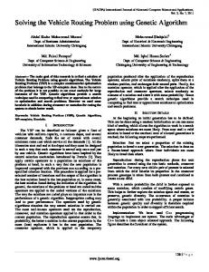
Distance: !5

10

8

Distance: !1

Figure 2: This example demonstrates a case where using range based binning can improve the result. Diagram (a) shows two histograms belonging to different classes of networked applications. We wish to separate them from one another, meaning we wish to apply a binning on them such that the distance between the two histograms increases. In this case range binning, presented in part (b), achieves the goal and frequency binning, presented in part (c), makes the problem worse. based binning attempts to ensure that if the learning sample is combined into a single histogram, each bin will contain roughly the same quantity. To put it another way, we can say that frequency based binning attempts to split the domain so that, when the new histograms are combined, the variance between each bin is minimized. When evaluating a binning we can observe how it affects classifications. A better binning will bring histograms representing the same class closer together, while separating those of different classes. A simple classification method is nearest neighbor classification. Using this method we calculate the euclidean distance between two histograms to decide how similar they are. Thus, if we have two histograms A and B with N bins each, we can define the distance between them as: ! "i