a GPU-Accelerated Implementation of the Cox Method

This article has been accepted for publication in a future issue of this journal, but has not been fully edited. Content may change prior to final publication. Citation information: DOI 10.1109/JSTSP.2016.2601820, IEEE Journal of Selected Topics in Signal Processing

IEEE JOURNAL OF SELECTED TOPICS IN SIGNAL PROCESSING

1

Effective connectivity analysis in brain networks: a GPU-Accelerated Implementation of the Cox Method Vafa Andalibi, Francois Christophe, Teemu Laukkarinen, Tommi Mikkonen

Abstract— The observation of interactions between neurons of a network can reveal important information about how information is processed within that network. Such observation can be established with the analysis of causality between the activities of the different neurons in the network. This analysis is called effective connectivity analysis. However, methods for such analysis are either computationally heavy for daily use or too inaccurate for making reliable analyses. Cox method produces reliable analysis, but the computation takes hours on CPUs, making it slow to use on research. In this paper, two algorithms are presented that speed up analysis of Cox method by parallelizing the computation on a Graphical Processing Unit (GPU) with the help of Compute Unified Device Architecture (CUDA) platform. Both algorithms are evaluated according to network size and recording duration. The interest of proposing GPU implementations is in gaining computation time but another important interest is that such implementation requires rethinking the algorithm in different ways as the sequential implementation. This rethinking itself brings new optimization possibilities, e.g. by employing OpenCL. Utilizing this accelerated implementation, the Cox method is then applied on an experimental dataset from CRCNS in a personal computer. This should facilitate observations of biological neural network organizations that can provide new insights to improve understanding of memory, learning and intelligence 1. Index Terms—Parallel algorithms, Parallel processing, Maximum likelihood estimation, Biological neural networks, Complex networks, Topology analysis

I. INTRODUCTION The observation of biological neural networks organizations plays a significant role in the development of innovative Paper submitted for review on October 31th 2015. “This work is supported by the Academy of Finland under Project: Bio-Integrated Software development for Adaptive Sensor Networks, project number 278882”. V. Andalibi is with Department of Electronics and Communications and Department of Pervasive Computing, Tampere University of Technology, PO Box 553, FI-33101 Tampere, Finland (e-mail: [email protected]). F. Christophe is with Department of Pervasive Computing, Tampere University of Technology, PO Box 553, FI-33101 Tampere, Finland (e-mail: [email protected]). T. Laukkarinen is with Department of Pervasive Computing, Tampere University of Technology, PO Box 553, FI-33101 Tampere, Finland (e-mail: [email protected]). T. Mikkonen is with Department of Pervasive Computing, Tampere University of Technology, PO Box 553, FI-33101 Tampere, Finland (e-mail: [email protected]).

topologies of Spiking Neural Networks (SNNs) [1], that are computationally more powerful than Artificial Neural Networks [2]. The non-linear dynamicity of neuronal networks within the neuroanatomical substrate (structural connectivity) of complex nervous systems, e.g. brain, produces patterns of statistical dependencies as well as causal interactions [3]. The former, i.e. functional connectivity, captures the statistical dependencies among spatially remote neurophysiological events and the latter, i.e. effective connectivity, explains the causal effects of a neural system over another [4]. The functional analysis of neural connections [5], [6] and connection changes [7] takes an important part in this observation for two reasons. First, this analysis enables the observation of causal relations between input stimuli and the activation of paths in a neural network, thus uncovering response patterns to specific events. Second, this analysis enables the creation of a strong relation between the structure of a network and its functionality. Based on the hypothesis of a strong correlation between network’s function and its structure, the analysis of temporal connectivity between neurons can be used to reproduce networks exhibiting complex functionalities such as face recognition, natural language processing or complex tasks requiring deep machine learning [8]–[11]. However, accurate methods for effective connectivity analysis, such as methods based on Maximum Likelihood (ML) estimation, are computationally expensive [12], [13]. Running such analysis on a personal computer typically requires hours of computing. This slows down the development of novel ideas inspired from such analysis of the complex behavior of biological neural networks. Compromising the accuracy of effective connectivity analysis with simpler methods for faster computation can lead to important misconceptions. For example, the Cross-Correlation Functional analysis (CCF) [14], a computationally simpler method than ML estimates, cannot recognize direct and indirect paths between two nodes of a network [15], whereas ML estimation based Cox method can [16]. Graphical Processing Units (GPUs) are not only capable of massive parallelization and crunching but also have very high energy efficiency compared to CPUs. The Compute Unified Device Architecture (CUDA) gives the possibility to execute parallel programs on a personal computer or a laptop GPUs. This provides High Performance Computing to a wider

1 Copyright (c) 2016 IEEE. Personal use of this material is permitted. However, permission to use this material for any other purposes must be obtained from the IEEE by sending a request to [email protected]

1932-4553 (c) 2016 IEEE. Personal use is permitted, but republication/redistribution requires IEEE permission. See http://www.ieee.org/publications_standards/publications/rights/index.html for more information.


IEEE JOURNAL OF SELECTED TOPICS IN SIGNAL PROCESSING population of researchers from disciplines such as bioinformatics [17]–[19]. This paper proposes two parallel algorithms for accelerating the Cox method [16] and compares the GPU-accelerated implementations of these algorithms according to two parameters: the number of neurons in the network (network size), and the length of neuronal activity recordings (recording time). These two implementations avoid compromising accuracy over execution time while enabling its execution on a personal computer. The difference between these algorithms lies on their better performance either over larger number of neurons in the network, or longer recording time of the network’s activity. While the first algorithm is more robust to longer recordings, the generally faster second algorithm suffers from limitations on it. This paper is organized as follows. First, the related works are presented through an overview of methods for effective connectivity analysis, a brief review of GPU implementations for the computational methods (ML estimates and Granger Causality Analysis [20]), and a presentation of the Cox method with its benefits. Second, as method for parallelizing a sequential algorithm, a representation of the sequential computation of the Cox method is analyzed. Two parallel implementations are proposed. The method for comparing these two implementations is also presented. Third, results of the evaluation of these two implementations are presented. Fourth, the Cox method is applied on an experimental dataset from Collaborative Research in Computational Neuroscience (CRCNS2). Fifth, discussion recommends one of these implementations depending on network size and recording time parameters. Finally, conclusions are given on the benefits of implementing the Cox method with CUDA and how this method should provide new insight for the development of novel architectures of SNNs. II. RELATED WORKS This section is organized in three parts. First, an overview of methods used for the analysis of neuronal effective connectivity presents the superiority in accuracy of Granger causality

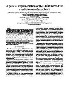
Figure 1 - Representation of spike trains of 10 simulated regular spiking neurons recorded for a duration of 1 second, produced with BRIAN [21] 2

2

1

2 3

1

2 3

Figure 2 - Example of two connectivity that pairwise methods cannot differentiate but can be recognized by both ML estimation methods and Granger causality analysis, adapted from [15].

analysis (GCA) and of methods based on ML estimation, as the Cox method. Second, a review of GPU implementations of ML estimates is given. In this part, it is noticed that none of the implementation found is applied to the study of the effective connectivity of neurons. Third, the Cox method is presented along with justifications of this choice of method for GPU implementation. A. Work related to connectivity analysis Effective connectivity analysis corresponds to the analysis of the temporal causality between the different activations of neurons on the network. Such analysis aims at creating connections between neurons based on their history of common activations forming a chain of events. For a neuron, an event is detected as a peak of a sudden depolarization of the electrical potential of the membrane. This brief peak is called a spike. The recording of the spikes of a neuron over time is called a spike train. Figure 1 shows spike trains of 10 spiking neurons, simulated with BRIAN simulator [21], and recorded for a period of 1 second. Spikes are simplified as instants in time due to their brief duration. Various methods are available for the analysis of effective connectivity of neural networks as presented in [4], [22]. However, only few of them are efficient in the analysis of effective connectivity as they can distinguish the connectivity difference between the two networks presented in Figure 2. The Cox method satisfies criteria of being non-pairwise, statistical and binless [6], [23]. Therefore, it is preconized for offline study of network connectivity as it provides robust results [7]. The following section presents works related to the parallelization of ML estimations and GCA methods. B. Work related to parallelizing ML and GCA methods: GPU-accelerated implementations have gained recent interest in neuroscience mostly for the simulation of models of spiking neurons. Rossant et al. have used a fitness function and a swarm optimization method implement on GPU to fit models of spiking neurons with electrophysiological recordings [24] instead of model fitting techniques based on ML estimates such as in [25], [26]. GPU parallelization is also used in accelerating likelihood function in phylogenetic inference [27]. Krömer et al. have accelerated an estimate of Hebbian learning with ML on GPU and naturally applied it to principal component analysis [13]. Shi et al. [28] address the GPU application in neural circuit mapping and electrophysiological data processing. In [29], Cao

www.CRCNS.org




3 𝑛

𝜑𝐴 (𝑡) = 𝜑𝐴 (𝑈𝐴 (𝑡)). 𝑒 ∑𝑖=1 𝛽𝑖𝑍𝐵𝑖 (𝑡)

Figure 3 - Simple spike train of three spikes and corresponding ISIs 𝒙𝟏 , 𝒙𝟐 and 𝒙𝟑 .

(1)

In (1), 𝑈𝐴 (𝑡) represents the duration since the last spike of neuron A. Most importantly, the parameters of interest for this connectivity analysis are 𝛽𝑖 as they represent the respective strength of connection from neuron Bi to A. 𝑍𝐵𝑖 (𝑡) represents an influence function of Bi on A defined as follows: 𝑗 𝑗 𝑘 𝑈 (𝑡−𝛥) 𝑈 (𝑡−𝛥) (2) 𝑔𝑚 − 𝐵 − 𝐵 𝜏 𝜏𝑟 𝑠 𝑍𝐵 (𝑡) = ∑ (𝑒 −𝑒 ) (𝜏𝑠 − 𝜏𝑟 ) 𝑗=1

where 𝑔𝑚 normalizes the maximum of the influence function to one and parameters and is defined as:

𝑔𝑚 = Figure 4 - Spike train of Figure 3 sorted in ascending order based on length of ISIs and addressed as new values 𝒙(𝟏) , 𝒙(𝟐) and 𝒙(𝟑) . The 𝒕𝒙(𝒊)𝒙(𝒋) values resulted by allocating smaller ISIs inside the larger ones ( i ≥ j ), coinciding left ends and considering right end of 𝒙(𝒋) as the t value.

et al. propose a GPU-implemented connectivity analysis solution to mine spike train datasets using frequent episode method. However, the robustness of the data-mining method should be the object of a comparative study with robust methods for effective connectivity analysis such as ML estimations. Statistical analysis tools running on GPU are also available as an open source package developed for R, the statistical environment used in biomedical research [22] and in particular this package contains a GPU implementation of GCA. This brief overview of GPU implementations of ML estimations reveals that GPU-acceleration has not yet drawn researchers’ attention for effective connectivity analysis in neuronal networks. Similarly, although Cox method is shown to be robust to, for instance, the analysis of non-linear processes, no GPU implementation of it the have been proposed so far to the knowledge of the authors. C. Presentation of the Cox method The Cox method [5] was initially presented for the analysis of multivariate point processes in signal processing. Borisyuk et al. show in [30] that such analysis is particularly fit for the analysis of neural network signals as Figure 2 shows an example of multivariate point processes based on the simulated activity of 10 neurons. This method is based on the assumption of the renewal of a spike on a spike train being modulated by other spike trains of the network, the modulated renewal process (MRP). This MRP is modeled in [6] and [31] as a hazard function expressing the probability of a spike rate at time t relatively to all inter-spike intervals (ISIs) of a spike train of length t or more. Considering a network of size n+1, the proportional hazard function of spike train of neuron A, 𝜑𝐴 (𝑡), is modulated in this model by the possible influence of other spike trains from other neurons Bi of the network as in:

𝑒

𝑡 − 𝑚 𝜏𝑠

𝑡 − 𝑚 𝜏𝑟

− 𝑒 𝜏𝑠 − 𝜏𝑟

(3)

In 𝑔𝑚 formula, 𝑡𝑚 is defined as: 𝑡𝑚 =

log(𝜏𝑠 − 𝜏𝑟 ) 1 1 − 𝜏𝑟 𝜏𝑠

(4)

where 𝜏𝑠 and 𝜏𝑟 defines the time of decay and rise of postsynaptic potential respectively, considered as 10 ms and 0.1 ms respectively. Using these exact values for 𝜏𝑠 and 𝜏𝑟 in Equation (3) and (4), 𝑡𝑚 and 𝑔𝑚 will be calculated as 0.4652 𝑗 and 0.0955 respectively. 𝑈𝐵 is the backward recurrence time of the process B with k as the index of the highest order of the backward recurrence time, i.e. the farthest from the moment 𝑡 − 𝛥. Here 𝛥 represents the propagation delay from reference neuron B to target neuron A which can be considered as 0. The exponential term of Equation (1) is estimated with the computation of a log likelihood function 𝐿(𝛽⃗) where 𝛽⃗ is the vector of 𝛽𝑖 of the hazard function in Equation (1). This likelihood function 𝐿(𝛽⃗), expressed as Equation (5), considers that the shortest ISIs between spikes has the highest contribution in connectivity between neurons as described in [7]. ⃗⃗) L(β

m

n

= ∑ ∑ βi . ZBi (t kk ) i=1 k=1 n

n

(5)

m

− ∑ log {∑ exp (∑ βi . ZBi (t lk ))} k=1

l=k

i=1

In Equation (5), m represents the number of neurons potentially having an influence on the activity of the neuron observed; n represents the number of spikes recorded for the study. With a spike train sorted based on the length of its ISIs and ∀k < 𝑙 (𝑙 and k are indices of an ISI), 𝑡𝑙𝑘 is calculated as right end of the kth ISI whilst it is inserted inside the lth ISI in a way that their left ends coincide. This sorting process is presented with the example of a spike train of 3 spikes as in



IEEE JOURNAL OF SELECTED TOPICS IN SIGNAL PROCESSING Figure 3, for which ISIs are sorted in Figure 4. Finding the maximum of 𝐿(𝛽⃗) implies finding the estimate 𝛽̂ of 𝛽⃗ such that: ⃗∇⃗𝐿(𝛽̂ ) = ⃗0⃗

(6)

Multivariate newton’s method is used for calculating the estimate of Equation (6). Newton’s method requires both the first and the second derivatives of log-likelihood. The first derivative is defined as in Equation (7): ⃗⃗𝐿(𝛽̂ ) ∇ 𝑛

= ∑ 𝑍𝐵𝑚𝑖𝑖 𝑖=1 𝑛

−∑[

∑𝑛𝑙=𝑖 𝑍𝐵𝑚𝑙𝑖 exp(∑𝑝𝑚=1 𝛽𝑚 𝑍𝐵𝑚𝑙𝑖 )

𝑖=1

∑𝑛𝑙=𝑖 exp(∑𝑝𝑚=1 𝛽𝑚 𝑍𝐵𝑚𝑙𝑖 )

(7) ]

(m=1,2,…,p) The formula for the second derivative, aka Hessian, is expressed as: (8) 𝜕2𝐿 𝜕𝛽𝑟 𝜕𝛽𝑠 𝑛 ∑𝑛𝑖=1 𝑍𝐵𝑟𝑙𝑖 𝑍𝐵𝑠𝑙𝑖 exp(∑𝑝𝑚=1 𝛽𝑚 𝑍𝐵𝑚𝑙𝑖 ) = ∑[ ] ∑𝑛𝑙=1 exp(∑𝑝𝑚=1 𝛽𝑚 𝑍𝐵𝑚𝑙𝑖 ) 𝑖=1 𝑛

− ∑[

∑𝑛𝑙=𝑖 𝑍𝐵𝑟𝑙𝑖 exp ∑𝑝𝑚=1 𝛽𝑚 𝑍𝐵𝑚𝑙𝑖 ∑𝑛𝑙=1 ZBsli exp(∑𝑝𝑚=1 𝛽𝑚 𝑍𝐵𝑚𝑙𝑖

𝑖=1

(r,s=1,2,…p)

𝑝

[∑𝑛𝑙=𝑖 exp(∑𝑚=1 𝛽𝑚 𝑍𝐵𝑚𝑙𝑖 )]

2

]

The main benefit of this method compared with other ML estimates is that it does not rely on a bin, i.e. a time window used for analyzing spike trains. However, as described in [6], [7], methods for solving Equation (6) using Equation (7) and (8) require computing the influence function 𝑍𝐵𝑖 (𝑡) for several values of t, depending on the number of neurons in the network

4

but also depending on the number of ISIs of the target neuron. Moreover, after calculating the values of influence function for all neurons, computation of Hessian (Equation (8)), is highly intensive computationally. The following chapter presents the two algorithms implemented in this paper for parallelizing these several computations of the function 𝑍𝐵𝑖 (𝑡). III. METHOD First, this section presents a representation of a sequential algorithm for computing the variables of connectivity strength of the Cox method 𝛽̂ as well as confidence intervals for these estimates. This representation enables finding the tasks that require parallelization. Secondly, a first parallel implementation with CUDA of this algorithm is presented with the parts dedicated for GPU computation. The main aspect of this implementation resides in using a GPU block for computations related to a certain spike timing of the target neuron. Thirdly, a second parallel implementation with CUDA considers using a GPU block computations related to a specific reference neuron. Finally, the method used for testing and evaluating the efficiency of execution of these two implementations is presented. The python codes and CUDA kernels are uploaded and available in GitHub3. A. Component Analysis of Cox method for Parallel Implementation The computation of the estimates coefficients of connectivity ̂ 𝛽 with the Cox method is represented with the pseudocode in Algorithm 1 as well as the sequential flow chart of Figure 5. The flowchart shows that heavy computations of first and second differentials of the log likelihood function are embedded inside three loops. It is noticed from this representation that first and second differential computations are independent tasks, and thus, can be parallelized. However, this optimization should have of much smaller effect than optimizing the availability of data necessary for the

Define reference neuron as r For each r Calculate ISI For each r For each target_spike (i) For each target_spike (j) if j 0.0001 Calculate the first derivative of log-likelihood Calculate the second derivative (Hessian) Calculate the new betahat values Calculate the confidence interval of betahat values

Algorithm 1 - Pseudocode of the computation of the betahats and corresponding confidence interval for a target neuron based on its reference spike trains. 3

https://github.com/Vafa-Andalibi/CUDA_Cox




5

Figure 6 - Simple network topology considered as example for describing the two GPU accelerated implementations of the Cox method.

computing the Cox method on only 1 neuron requires the computation of 536870912 values (10243/2) of the influence function 𝑍() . This example shows the importance of accelerating this computation with GPU, as parallelizing these computations should save a significant amount of time on executing the Cox method. The following sections describe these two implementations in more details by taking the network structure of Figure 6 as an example. In this example, the values of connectivity from reference neurons 1 and 2, 𝛽̂ , are computed for the target neuron. Each neuron is considered spiking three times similarly to the representations of Figure 3 and Figure 4. The influence function 𝑍() should be computed for each reference neuron at each spiking time of the target neuron. This simple network topology helps clarifying the structure of these implementations and expressing the computations handled in each thread of the GPU blocks. Figure 5 - Flow chart of the main tasks of the Cox method presented sequentially. The notations dL1 and dL2 in this chart correspond to the first and second differential of the log ⃗⃗⃗. likelihood L according to the coefficients of connectivity, 𝜷 Thus, dL1 corresponds to the gradient of the log likelihood and dL2 corresponds to the Jacobian of this gradient, also called the Hessian matrix of the log likelihood.

computation of these two differentials. Indeed, the expression of the first and second differentials as derived from Equation (5), shows the importance of computing the values of the influence function 𝑍𝐵𝑖 (𝑡) from all neurons and at all their spiking times. The key approach for the two parallel implementations proposed in this paper is to use the blocks and their corresponding threads of GPU to compute all the values of 𝑍𝐵𝑖 (𝑡𝑙𝑘 ) in parallel. The number of values that need to be computed for analyzing the connections from the rest of the network to one of its neuron equals n.m2, provided that the network as n+1 neurons of which m spikes have been recorded. Considering, for instance, a network of 1025 neurons with a recording time corresponding to a collection of 1024 spikes,

B. Algorithm dedicating each GPU block to a specific spiking time of the target neuron This algorithm gathers the Z values of all reference neurons for a specific spiking time of the target neuron into the same GPU block. Each thread of that block computes the value of influence of a reference neuron at that specific time, as depicted in Figure 7. This specific timing results from sorting as illustrated in Figure 4. As each block calculates the values of Z for a unique time, 𝑡𝑥(𝑖)𝑥(𝑗) , but for all reference neurons, the number of blocks in this algorithm will not grow with an increase of number of neurons in the network. Hence, the performance will not face a significant deterioration, as the second algorithm’s will, by increasing the number of neurons. In this implementation, a block always contains n threads, with n+1 being the number of neurons in the network. The GPU grid contains blocks where m is the number of ISIs of the target neuron. C. Algorithm dedicating each GPU block to a reference neuron and the first index of target spiking time This algorithm positions the values to be computed on the GPU grid as described in Figure 8. A row of this grid




6

Figure 7 - Schematic of the grid formation for the first algorithm where 𝒁𝒓𝒆𝒇 𝒏 (𝒕𝒊𝒋 ) indicates the Z value of reference neuron n at time 𝒕𝒊𝒋 .

Figure 8 - Schematic of the grid formation for the second algorithm where 𝒁𝒓𝒆𝒇 𝒏 (𝒕𝒊𝒋 ) indicates the Z value of reference neuron n at time 𝒕𝒊𝒋 .

corresponds to the Z values related to a specific reference neuron. A column corresponds to a specific target time. Therefore, threads of a same block will always contain Z values of the same reference neuron (e.g. ref1) and have the same value for the first index of tij (e.g. t3j). The threads of a block compute all the Z values for that specific time with consideration to all the smaller ISIs inside this specific time, i.e. 𝑍𝑟𝑒𝑓𝑛 (𝑡𝑖𝑗 ) with 𝑗 ≤ 𝑖. In this algorithm, the grid size is then 𝑛 × 𝑚, and a block contains m threads. The grid size will grow linearly with the growth of ISIs as well as with the growth of neurons.

experiment, the animal is rewarded with water. This specific dataset was recorded for a duration of 1096.4 seconds with sampling rate of 20 KHz. The recording was performed using 4 electrodes (shanks) each with 8 recording sites. After the processing and spike sorting of the raw data, the spikes that seem to be generated by the same neuron are placed into the same category (cluster). Note that number of clusters for each electrode could be different from number of recording sites, as illustrated in Table 1. Furthermore, it is of significance that the exact number of spikes per cluster varies a lot in each cluster. As shown in Table 2, number of spikes per each cluster recorded by E4, varied between 51 and 107340.

D. Testing method Algorithms were tested for computational time efficiency in two steps. First, we compared them with CPU sequential implementation (2 variables of comparison: number of neurons, avg. number of spikes in trains). Second, we compared the algorithms against each other with the same comparison criteria. The number of neurons in the network on which algorithms were tested varies from 4 to 64 in the case of evaluation against CPU, and from 64 to 256 in the comparison of the two parallel implementations. The duration of recording for tests varies from 20s to 40s in test against CPU (with 24 neurons in the network) and from 20s to 52s for the evaluation of parallel implementations (with 64 neurons in the network). E. Experimental Data The GPU accelerated Cox method was applied on a real dataset downloaded from CRCNS database. The selected dataset, entitled hc3, contains recordings from various hippocampal regions of a rat. Each part of this dataset is dedicated to a specific behavioral task of the animal, such as running on a wheel, an Mwheel, a big square, or a Tmaze. In this study, the Cox method is applied on neuronal activity during the selected behavioral task named Mwhell. Thus task corresponds to an alternation task in T-maze (100cm x 120cm) with wheel running delay [32]. In this task, the animal first runs on a wheel attached to a waiting area. Then, after 10 seconds, the animal is released to the central arm of a T-maze. At the end of this arm, the animal can choose whether to go to left or right. In case of selecting the opposite direction than in previous

Table 1 - Number of clusters and average number of spikes per cluster in each electrode.

Electrode Index

Number of Clusters

Average number of spikes per Cluster

E1

9

9905.33

E2

11

12298.91

E3

10

13752.4

E4

4

33905

Table 2 - Number of spikes per cluster in E4

Cluster Index

C1

C2

C3

C4

Number of Spikes

51

107340

1179

27050

IV. RESULTS The sequential implementation of the Cox method was developed and executed with Matlab. In order to propose a fair comparison between CPU and GPU, the initial Matlab implementation provided by [6], was analyzed with Matlab




Figure 9 Comparison of execution times of the 3 Cox method implementations, as variable of the number of neurons in the network. The illustrated values are CPU runtime duration divided by corresponding GPU duration.

profiler and bottlenecks were optimized. In addition, this Matlab implementation was executed using a local parallel pool of four workers (with the use of parfor loops). The maximum possible workers on a local parallel pool is equal to number of cores of the CPU, hence the four workers for a Core i7 CPU. The Matlab profiler confirmed that over 95% of the processing time is spent on calculating the Z-values and Hessian. This parallelized Matlab version of Cox method is also made available on GitHub4. As for the GPU implementations, PyCUDA library was used to compile CUDA kernels in the python code. The experimental platform is a laptop equipped with an Intel Core i7-4702MQ CPU and NVIDIA GK208M (Geforce 740M GT) with 2 GB video memory. The results are presented in two sections. First, the difference of performance between CPU and GPU implementations is shown. Second, the performance of both algorithms is compared according to the two important parameters of activity recording: network size, and recording duration.

Table 3 - Duration of Z-values and Hessian calculation as well as total runtime in CPU implementation for networks of size 4 to 64 at a fixed recording duration of 25 seconds. Number of Neurons 4 8 16 24 32 40 48 56 64 4

Average number of spikes 396.5 392 410 403.7 421.3 419.9 401.3 417.9 424.3

Z-values calculation duration [s] 3.18 11.64 46.13 100.9 187.8 290.08 394.86 555.47 819.67

Hessian calculation duration [s] 9.789 35.78 162.68 458.56 1023.79 1843.23 3139.59 5115.94 8251.8

7

Figure 10 Comparison of execution times of the 3 Cox method implementations, as variable of the duration of recording. The illustrated values are CPU runtime duration divided by corresponding GPU duration.

A. Evaluation against CPU 1) Evaluation of execution time GPU algorithms and CPU runtimes are compared with regard to duration of recording, i.e. train lengths, and number of neurons. The network in the former test consists of 24 neurons and the duration of the recording varies from 20 seconds (average of 352.13 spikes per train) to 40 seconds (average of 656.67 spikes per train). In the latter test, size of the network was realized with networks containing from 4 to 64 neurons at a fixed recording duration of 25s (duration equivalent to an average of 424 spikes per neuron). The runtime duration of both tests in CPU are presented in Table 3 and Table 4 respectively. Overall, these measurements, presented in Figure 9 and Figure 10, show an average ten times speedup for both GPU implementations compared to the optimized parallel Matlab implementation. The following subsections evaluate the precision evaluation as well as performance of GPU implementations on larger datasets. 2) Evaluation of precision As a trade-off to CPU computing precision with 64 bits floating points (FP64), GPU implementations uses only 32 bits floating points (FP32). The connectivity results from CPU and GPU algorithms as presented in Figure 11 and Figure 12 show a Table 4 - Duration of Z-values and Hessian calculation as well as total runtime in CPU implementation at recording duration of 20 to 40 seconds for network size of 24 neurons.

Total duration [s]

Recording Duration [s]

13.81 50.61 221.05 586.66 1260.58 2208.11 3637.26 5813.326 9276.95

20 22.5 25 27.5 30 32.5 35 37.5 40

Average number of spikes 325.13 366.71 408.25 450.88 492.13 533.62 573.92 616.17 656.67

Z-values calculation duration [s] 63.61 80.262 100.706 124.17 151.332 178.077 212.99 250.9 294.598

Hessian calculation duration [s] 294.16 363.029 450.444 525.542 631.256 735.57 813.472 929.592 1078.252

Total duration [s] 378.523 466.543 578.036 679.941 817.093 945.095 1068.565 1227.069 1425.304

https://github.com/Vafa-Andalibi/CUDA_Cox/tree/master/CPU_Matlab




a)

Neuron 1 Index

Neuron Index

1

2

3

4

0.817134863426029 0 0.924795560858616 0.156808705640583

2

3

0 0 0 -0.571694815927135 0.381791637882763 0 -0.319917476791795 0.500488765395997 0 -0.266158057663006 0.501723627603362

1

c)

3

0 -0.094951589022186 0.090285644302101 0.117782784970178

1 2 3 4

b)

2

from

to

2 3 2 3

1 1 3 4

0.462930542512753 1.171339184339306 0 0 0 0 0.573917479447795 1.275673642269438 0 -0.246735503450937 0.560352914732103

8 4

0.719542805555054 -0.122409007772366 0 1.081090826536209

-0.035954401625954 -0.162761838593228 -0.132307868924232 0

4 0.366858879975739 1.072226731134368 0 -0.608763479211233 0.363945463666501 0 0 0 0 0.768056390272881 1.394125262799536

-0.438165412498214 0.366256609246306 0 -0.635801678018669 0.310278000832213 0 -0.585630552294384 0.321014814445920 0 0 0

0.817134863426029 0.719542805555054 0.924795560858616 1.081090826536209

Figure 11 Output of CPU implementation of Cox method in a network of 4 neurons and 25 second of recording duration. a) Adjacency matrix of Cox coefficients (betahat) b) Adjacency matrix of confidence intervals for Cox coefficients. If the confidence interval does not contain zero, it is considered as a connection and the corresponding Cox coefficient is considered as strength of connection (bold numbers), c) Connectivity result of the network with Cox coefficients as strength of connection

precision loss of 0.046% to 0.048% for each value in these figures.

a) Neur on I ndex

1 2 3 4

1

[[ [ [ [

2

0. - 0. 09499713 0. 09032792 0. 1178383

3

4

0. 8175219 0. 71988346 - 0. 035972 ] 0. - 0. 12246726 - 0. 16283952] 0. 92523407 0. - 0. 13237104] 0. 15688086 1. 08160367 0. ]]

b) Neur on 1 I ndex

[[ [ [ [ 2 [ [ [ 3 [ [ [ 4 [ 1

0. 0. 0. - 0. 0. 0. - 0. 0. 0. - 0. 0.

2

57196818 38197392 32006992 50072575 2662851 5019617

3

4

0. 46315142 0. 36703387 - 0. 43837478] 1. 17189237 1. 07273305 0. 36643078] 0. 0. 0. ] 0. - 0. 60905269 - 0. 63610522] 0. 0. 36411818 0. 31042618] 0. 0. 0. ] 0. 57419195 0. - 0. 58591005] 1. 27627619 0. 0. 32116797] 0. 0. 0. ] - 0. 24685837 0. 76842363 0. ] 0. 5606201 1. 39478371 0. ]]

c) f r om [[ [ [ [

2. 3. 2. 3.

to 1. 1. 3. 4.

0. 0. 0. 1.

8175219 ] 71988346] 92523407] 08160367] ]

Figure 12 Output of both GPU-accelerated algorithms for Cox method in a network of 4 neurons and 25 second of recording duration. a) Adjacency matrix of Cox coefficients (betahat), b) Adjacency matrix of confidence intervals for Cox coefficients. If the confidence interval does not contain zero, it is considered as a connection and the corresponding Cox coefficient is considered as strength of connection (bold numbers), c) Connectivity result of the network with Cox coefficients as strength of connection

B. Evaluation of GPU algorithms Similar to the preliminary evaluation against CPU, the evaluation of the two accelerated implementations is realized on network size and recording time criteria. However, this evaluation observes differences between GPU-accelerated implementations with larger datasets than preliminary. The focus of evaluation is placed on the Z value calculation, Hessian calculation, memory copy from Device to Host (DtoH) and Host to Device (HtoD), device occupancy as well as total calculation time. The first evaluation is based on network sizes ranging from 64 to 256 neurons at a constant recording time of 25s (equivalent to an average of ~350 spikes per recorded neuron) as presented in Figure 13. As a general observation for both curves presented in this figure, both algorithms seem to grow linearly with network growth. The implementation presented in III.C (Alg.2) performs faster than the one described in III.B (Alg.1). The time required for DtoH and HtoD memory copy in both algorithms are alike. The second evaluation is based on a network of 64 neurons recorded for durations ranging from 20s to 52s. (equivalent to average spikes per neuron ranging from 325 to 844). Results from this evaluation can be observed from Figure 14. In this test case, although Alg.1 takes longer than Alg.2, the latter runs out of memory with block size bigger than 1024 threads (NVIDIA GK208M thread per blocklimit) as the size of GPU grid grows with the number of spikes. Similar to previous test, the memory transfer time (DtoH and HtoD) in both algorithms are almost identical. Despite the fact that Alg. 1 is slightly slower than Alg. 2, the total computation time of both algorithms in both tests are very




Figure 15 Comparison of Hessian and Total execution times between the 2 GPU implementations of the Cox method, as a variable of the number of neurons in the studied network.

similar, as illustrated in Figure 15 and Figure 16. Note that the required time for hessian calculation, which is also parallelized on GPU, is almost indistinguishable since both uses the same algorithm. Moreover, for both algorithms the ratio between total execution times (Figure 15 and Figure 16) and memory transfer as a summation of both DtoH and HtoD (Figure 13 and Figure 14) is on average 25 in the first scenario, i.e. with a variable of the number of neurons in the studied network, and 18 in the second scenario, i.e. with a variable of the average number of recorded spikes in the studied network. Regarding the device occupancy, the occupancy of Alg.1 increases by enlarging the number of neurons in the network as is shown in Figure 17. This describes the steady occupancy of 50% in Figure 18 as the number of neurons is constant (64). Conversely, the device occupancy in Alg.2 increases by number of spikes, which is the reason of its high occupancy in both tests since the minimum spike of both tests are about 350 spikes.

9

Figure 16 Comparison of execution times between the 2 GPU implementations of the Cox method, as a variable of the average number of recorded spikes in the studied network.

effect on spiking of the target cluster i. The strength of connection is measured as follows: first, the whole spike trains with length of 1096400 ms is trimmed into windows of length 15,000 ms with an overlap of 100 ms. The Cox method is then applied on each of these windows. Having the Cox method indicating connections, a circle is drawn in the corresponding cell based on the target and reference cluster index. In case the connection was already found in previous window(s), the radius of the circle is increased. For instance, the strength of the connection from C3 in E1 to C1 in E1 is less than that of C8 in E1 to C8 in E3. This result can also be illustrated in form of a directed graph, representing causality in the network. Figure 19 shows the final connection map. This figure clarifies that during the MWheel activity, the source of the majority of connections are cluster 3 and 8 in electrode 1 as well as cluster 1 in electrode 2, 3 and 4. V. DISCUSSION

C. Experimental Data Figure 20 illustrates the adjacency matrix resulting from the application of the GPU accelerated Cox method on the experimental data described in III.E. In this figure, a circle in row i and column j implies that the reference cluster j has an

Figure 11 and Figure 12 illustrates the output of the Cox method over a small network of 5 neurons. This output consists of three parts: adjacency matrix of beta values (Figure 11.a and Figure 12.a), adjacency matrix of confidence interval for beta values (Figure 11.b and Figure 12.b) and final connectivity

Figure 13 Comparison of Z-value and memory copy (device to host and host to device) times between the 2 GPU implementations of the Cox method, as a variable of the number of neurons in the studied network.

Figure 14 Comparison of Z-value and memory copy (device to host and host to device) times of between the 2 GPU implementations of the Cox method, as a variable of the average number of recorded spikes in the studied network.



IEEE JOURNAL OF SELECTED TOPICS IN SIGNAL PROCESSING results (Figure 11.c and Figure 12.c). The integrity of implementation of both CUDA algorithms in comparison with the CPU implementation was examined. Indeed, with identical dataset, all three algorithms produce identical effective connectivity results. An instance of Cox method as detailed in this paper only considers the computation of connectivity coefficient to one neuron of the network. Therefore, acquiring the network effective connectivity requires the method to be executed N times in a neural network of N neurons. For this reason, all runtimes of this study consider the duration needed for attaining the full connectivity of the network. Results from larger datasets definitely rule out the use of sequential implementation of the method. For instance, a network composed of 24 neurons with a recording duration of 40 seconds (an average of 656 spikes recorded per neuron requires) CPU takes ~5 min for computing Z values, ~18 min for computing the Hessian and ~24 min for acquiring the entire network connectivity, whereas GPU algorithms needs ~29.4 seconds for calculating Z values, less than 2 minutes for Hessian and 2 and a half minutes for whole connectivity. Similarly, test on a network of 64 neurons with 25 seconds of recording duration (each ~424 spikes) requires CPU 13 and a half min. for computing the Z values, 137 min for Hessian and ~157 min to compute entire network connectivity, whereas the first algorithm needs 74s. for each Z matrix, 13 min for Hessian and 14 minutes for full network connectivity. The performance of proposed algorithms for calculating the Z Values varies depending on the characteristic of the data. With a large number of neurons in the dataset, Alg.1 will eventually become slightly faster than Alg.2 in case the number of neurons in the networks exceeds the average number of recorded spikes. However, this algorithm is vulnerable against long spike trains in a network containing small number of neurons due to low occupancy of the device. In turn, Alg.2 is outperformed when the number of neurons increases, provided that the extensive number of neurons does not exceed the capacity of the RAM and GPU memory. These results can be applied on real datasets of up to 1024 neurons in first algorithm and up to 1024 spikes in each train in second algorithm.

Figure 17 Comparison of device occupancy between the two Z-Value kernels as well as the Hessian, as a variable of the number of neurons in the studied network.

10

Figure 19 Result of the Cox method applied on an experimental data for MWheel task in form of unweighted graph.

Respectively, there is a limit for number of spikes in each train and number of neurons in the network which is dependent on the memory of the GPU. Selecting an accelerated implementation preferably to the other depends on the number of neurons and the time of recording of the dataset. According to [7], the Cox method provides accurate results with recordings of 256 spikes (approximately 40 seconds recording). This limit marks a decisive point for the selection of an implementation preferably to another. Recordings need to last at least 20s. In case, recordings are longer, they can always be split into recording parts of 20s. minimum duration. Now let us assume the recording duration is 40s., which is equivalent to 512 spikes per neuron. Dealing with a dense network composed of more than 512 neurons, one shall choose Alg.1. In the contrary, Alg.2 is to be chosen when observing the activity of a network with fewer than 512 neurons.

Figure 18 Comparison of device occupancy between the two Z-Value kernels as well as the Hessian as a variable of the average number of recording duration in the studied network.




11

The selected experimental hc3 dataset from CRCNS contains a total of 32 neuron clusters recorded from 4 electrodes. Considering this small number of neuron clusters, it would be inefficient to apply the first proposed parallel algorithm on the dataset since at least 992 threads of each block would remain unused, hence the second algorithm is applied. There are some limits in utilizing the Cox method on experimental dataset as well. As illustrated in Table 2, some of the spike trains are very short in length compared to others, e.g. 50 spikes in 1096400 ms. Cox method cannot be applied on such train since for the method to achieve a correct asymptotic statistical level of 95% confidence, target trains need to have at least 256 spikes in it. Note that in our case, this problem persists even if the train length reaches that limit. An ideal solution would be for the train to have a train_length/window ratio of 256 spikes. VI. CONCLUSION In this paper, we analyzed the possibility of parallelizing the Cox method components and compared two parallel CUDAbased algorithms for accelerating the calculation of the values of the influence function Z(). These values can be represented in the form of a 3D matrix of size n × m × m. Moreover, the calculation of the Hessian of ML was also accelerated with GPU. In comparison with the Matlab implementation optimized and parallelized with parfor loops, the proposed GPU implementations show an improvement of an order of magnitude in execution time. The Cox method, formerly demanding a long time as well as consequent CPU power, can now run on CUDA-supported GPUs in personal computers. This implementation will certainly benefit a wide range of researchers in the fields of neural networks, neuroscience as well as neurobiology labs. Effective connectivity analysis gives the opportunity to observe and recreate networks structures directly inspired from natural structures, similarly to the Hierarchical Temporal Memory [33] or for reinforcement learning [34]. As opposite, considering the use of biological neural networks for computation tasks also represents a leap forward in cybernetics and in-terms of energy savings. Such solution becomes possible as biological feedforward neural networks have been developed [35]. This implementation is also advantageous with regard to interval of extracting connectivity map, making it possible to analyze effective connectivity evolution. With short run-time of Cox method it would be possible to calculate 𝑑𝛽/𝑑𝑡 to foresee the succeeding Beta values, facilitating the accurate control over stimulations for obtaining a defined topology. Hence, with a simultaneous employment of 𝑑𝛽/𝑑𝑡 and dynamic stimuli, a great precision is achievable. In this manner, controlling the plastic changes of a network could enable its engineering for specific cognitive tasks. In near future, the next version will be adapted to PyOpenCL in order to provide possibility for laptops without specialized hardware to benefit from these implementations. We also expect form this adaptation to show that it is the algorithms and not the GPU that bring a significant speedup. This assumption

Figure 20 Result of the Cox method applied on an experimental data for MWheel task in form of adjacency matrix.

will be tested. Other future developments consist in proposing an optimized parallel implementation for CPUs, for instance in C/C++ using OpenMP. Such implementation will allow an accurate comparison of execution speed of parallel CPU implementation and the GPU implementations proposed in this paper, as the comparisons applied in [36]. This parallel implementation for CPU will also provide the possibility to the research community to run computational methods on standard computers. ACKNOWLEDGMENT This research is funded by the Academy of Finland under project number 278882 – Bio-integrated Software Development for Adaptive Sensor Networks. REFERENCES [1]

J. Harkin, F. Morgan, L. McDaid, S. Hall, B. McGinley, and S. Cawley, “A Reconfigurable and Biologically Inspired Paradigm for Computation Using Network-On-Chip and Spiking Neural Networks,” Int. J. Reconfigurable Comput., vol. 2009, pp. 1–13, 2009.

[2]

K. J. Cios and M. E. Shields, “The handbook of brain theory and neural networks,” Neurocomputing, vol. 16, no. 3, p. 1083, 1997.

[3]

O. Sporns, D. R. Chialvo, M. Kaiser, and C. C. Hilgetag, “Organization, development and function of complex brain networks,” Trends Cogn. Sci., vol. 8, no. 9, pp. 418–425, 2004.

[4]

K. J. Friston, “Functional and effective connectivity: a review,” Brain Connect., vol. 1, no. 1, pp. 13–36, 2011.

[5]

D. R. Cox and P. A. W. Lewis, “Multivariate point processes,” in Sixth Berkeley Symposium, 1972, pp. 401–448.

[6]

M. S. Masud and R. Borisyuk, “Statistical technique for analysing functional connectivity of multiple spike trains,” J. Neurosci.




[7]

[8]

[9]

12

Methods, vol. 196, pp. 201–219, 2011.

[23]

T. Berry, F. Hamilton, N. Peixoto, and T. Sauer, “Detecting connectivity changes in neuronal networks,” J. Neurosci. Methods, vol. 209, pp. 388–397, 2012.

T. L. T. M. K. K. Francois Christophe Vafa Andalibi, Survey and evaluation of neural computation models for bio-integrated systems. Elsevier, 2015.

[24]

C. Rossant, D. F. M. Goodman, J. Platkiewicz, and R. Brette, “Automatic fitting of spiking neuron models to electrophysiological recordings.,” Front. Neuroinform., vol. 4, p. 2, 2010.

[25]

L. Paninski, J. W. Pillow, and E. P. Simoncelli, “Maximum likelihood estimation of a stochastic integrate-and-fire neural encoding model.,” Neural Comput., vol. 16, pp. 2533–2561, 2004.

[26]

L. Paninski, J. Pillow, and J. Lewi, “Statistical models for neural encoding, decoding, and optimal stimulus design,” Progress in Brain Research, vol. 165. pp. 493–507, 2007.

[27]

F. Pratas, P. Trancoso, L. Sousa, A. Stamatakis, G. Shi, and V. Kindratenko, “Fine-grain parallelism using multi-core, Cell/BE, and GPU systems,” Parallel Comput., vol. 38, pp. 365–390, 2012.

[28]

Y. Shi, A. V Veidenbaum, A. Nicolau, and X. Xu, “Large-scale neural circuit mapping data analysis accelerated with the graphical processing unit (GPU),” J. Neurosci. Methods, vol. 239, pp. 1–10, 2015.

[29]

Y. Cao, D. Patnaik, S. Ponce, J. Archuleta, P. Butler, W. C. Feng, and N. Ramakrishnan, “Parallel mining of neuronal spike streams on graphics processing units,” in International Journal of Parallel Programming, 2012, vol. 40, pp. 605–632.

[30]

G. N. Borisyuk, R. M. Borisyuk, A. B. Kirillov, E. I. Kovalenko, and V. I. Kryukov, “A new statistical method for identifying interconnections between neuronal network elements,” Biol. Cybern., vol. 52, pp. 301–306, 1985.

[31]

F. Hamilton, T. Berry, N. Peixoto, and T. Sauer, “Real-time tracking of neuronal network structure using data assimilation,” Phys. Rev. E, pp. 1–6, 2013.

[32]

E. Pastalkova, V. Itskov, A. Amarasingham, and G. Buzsáki, “Internally generated cell assembly sequences in the rat hippocampus,” Science (80-. )., vol. 321, no. 5894, pp. 1322–1327, 2008.

[33]

J. Hawkins, “Whitepaper: Hierarchical Temporal Memory including HTM Cortical Learning Algorithms.” p. 68, 2011.

[34]

T. H. Teng, A. H. Tan, and J. M. Zurada, “Self-Organizing Neural Networks Integrating Domain Knowledge and Reinforcement Learning,” IEEE Transactions on Neural Networks and Learning Systems, 2014.

[35]

A. Natarajan, T. B. DeMarse, P. Molnar, and J. J. Hickman, “Engineered In Vitro Feed-Forward Networks,” J. Biotechnol. Biomater., vol. 03, no. 01, pp. 1–7, 2013.

[36]

V. W. Lee, P. Hammarlund, R. Singhal, P. Dubey, C. Kim, J. Chhugani, M. Deisher, D. Kim, A. D. Nguyen, N. Satish, M. Smelyanskiy, and S. Chennupaty, “Debunking the 100X GPU vs. CPU myth,” ACM SIGARCH Comput. Archit. News, vol. 38, no. 3, p. 451, 2010.

K. Kavukcuoglu, P. Sermanet, Y.-L. Boureau, K. Gregor, M. Mathieu, and Y. LeCun, “Learning Convolutional Feature Hierarchies for Visual Recognition,” Adv. neural Inf. Process. Syst. 23, no. 1, pp. 1090–1098, 2010. C. Farabet, C. Couprie, L. Najman, and Y. Lecun, “Learning hierarchical features for scene labeling,” IEEE Trans. Pattern Anal. Mach. Intell., vol. 35, pp. 1915–1929, 2013.

[10]

J. Martens, “Generating Text with Recurrent Neural Networks,” Neural Networks, vol. 131, no. 1, pp. 1017–1024, 2011.

[11]

A. Graves, G. Wayne, and I. Danihelka, “Neural Turing Machines,” arXiv Prepr. arXiv1410.5401, 2014.

[12]

S. Yang and D. De Angelis, “Maximum likelihood.,” Methods Mol. Biol., vol. 930, pp. 581–95, 2013.

[13]

P. Krömer, E. Corchado, V. Snášel, J. Platoš, and L. GarcíaHernández, “Neural PCA and maximum likelihood hebbian learning on the GPU,” in Lecture Notes in Computer Science (including subseries Lecture Notes in Artificial Intelligence and Lecture Notes in Bioinformatics), 2012, vol. 7553 LNCS, pp. 132–139.

[14]

D. H. Perkel, G. L. Gerstein, and G. P. Moore, “Neuronal spike trains and stochastic point processes. II. Simultaneous spike trains.,” Biophys. J., vol. 7, pp. 419–440, 1967.

[15]

A. Seth, “Granger causality,” Scholarpedia, vol. 2, no. 7, p. 1667, 2007.

[16]

D. R. Cox and P. A. W. Lewis, “Multivariate point processes,” Sel. Stat. Pap. Sir David Cox Vol. 1, Des. Investig. Stat. Methods Appl., vol. 1, p. 159, 2005.

[17]

A. Bustamam, K. Burrage, and N. A. Hamilton, “Fast parallel markov clustering in bioinformatics using massively parallel computing on GPU with CUDA and ELLPACK-R sparse format,” IEEE/ACM Trans. Comput. Biol. Bioinforma., vol. 9, pp. 679–692, 2012.

[18]

A. A. Huqqani, E. Schikuta, S. Ye, and P. Chen, “Multicore and GPU parallelization of neural networks for face recognition,” in Procedia Computer Science, 2013, vol. 18, pp. 349–358.

[19]

S. Scanzio, S. Cumani, R. Gemello, F. Mana, and P. Laface, “Parallel implementation of Artificial Neural Network training for speech recognition,” Pattern Recognit. Lett., vol. 31, pp. 1302– 1309, 2010.

[20]

T. E. Society and C. W. J. Granger, “Investigating Causal Relations by Econometric Models and Cross-spectral Methods,” Econometrica, vol. 37, pp. 424–438, 1969.

[21]

D. F. M. Goodman and R. Brette, “The brian simulator,” Frontiers in Neuroscience, vol. 3. pp. 192–197, 2009.

[22]

J. Buckner, M. Seligman, and J. Wilson, “gputools: A few GPU enabled functions. R package.” 2011.

AUTHORS’ BIOGRAPHIES Vafa Andalibi obtained his Bachelor’s degree in Computer Engineering from Iran University of Science and Technology (IUST) in 2012. He received his double major master’s degree in Biomedical Engineering and Communication Systems and Networks from Tampere University of Technology in 2016. His research interests include parallel and distributed systems, computer networking, BioIntegrated Systems (BIS), computational neuroscience, neural modeling, neuron-computer interface and functional organization of neuronal circuits. He is currently a research assistant at University of Helsinki.

François Christophe received his bachelor in Signal processing and Automation from University of West Brittany (France) in 2004, and his Master degree in Computer and Software Engineering from Brest National Engineering School (France) in 2007. He received his Ph.D. degrees from Aalto University (Finland) and Nantes Centrale Engineering School (France) in 2012. He works currently as post-doctoral researcher in the Department of Pervasive Computing at Tampere University of Technology. His research interests include computational models and modeling methods for the integration of biological components in digital and software applications.




13

Teemu Laukkarinen (D.Sc. '15, M.Sc. '10) received M.Sc. in computer science in 2010 and D.Sc. in computer science in 2015 from the Tampere University of Technology (TUT). He is currently working as a post-doctoral researcher at the Department of Pervasive Computing at TUT. He has published several international peer reviewed journal and conference articles. His teaching expertise covers computer architecture, microcontroller systems, and wireless sensor network (WSN) applications. He co-founded a spin-off company from the WSN research of TUT in 2010. His main research interesets are embedded software, abstractions, machine learning, and bio-integrations in the domain of resource constrained Internet-of-Things. Tommi Mikkonen (M.Sc. 1992, Lic. Tech. 1995, Dr. Tech 1999, all from Tampere University of Technology, Tampere, Finland) works on software architectures, software engineering and open source software development at the Institute of Software Systems at Tampere U of Tech. Over the years, he has written a number of research papers, and supervised theses and research projects on software engineering. At present, he is working as the head of the Department of Pervasive Computing at TUT.


a GPU-Accelerated Implementation of the Cox Method

a GPU-Accelerated Implementation of the Cox Method

Suggest Documents

Implementation of a Robust Bayesian Method - Universidad ...

A parallel implementation of the LTSn method for a ... - CiteSeerX

A massively parallel GPUaccelerated model for analysis of fully ...

A massively parallel GPUaccelerated model for analysis of ... - DTU Orbit

implementation of the quadrature method of ...

Implementation of the Glucommander Method of

A Multi-Method Evaluation of the Implementation of

Numerical implementation of the factorization method ... - CiteSeerX

The Implementation of Group Method to Improve

A new method for the implementation of arbitrary ... - Semantic Scholar

A Parallel Implementation of the Davidson Method for ... - UPV

On the implementation of a method for automatic ...

Parallel Implementation of a Method on the Experimental G-\ Multigrid ...

Design and implementation of a method for the

COX

A Matlab Implementation of the Implicitly Restarted Arnoldi Method ...

Implementation of a Full P1 Method in the Diffusion ...

Critical Path Method Implementation Drawbacks: A Discussion ...

A Design and Implementation of a Snapshot Based Method for ...

Implementation of a Time-Domain Random-Walk Method into a ...

SCPS: a fast implementation of a spectral method for ... - BioMedSearch

A SLICOT Implementation of a Modified Newton's Method for ...

A method for assessing implementation success of a ... - Springer Link

Method of using of the Box-Cox transformation at the application of the ...