Idelsohn and Oñate [7] identify the main difficulties in mesh building as the need for a conforming mesh, in which all nodes must lie at element vertices, the need.
Boundary Elements and Other Mesh Reduction Methods XXXV
11
A GPU-accelerated meshless method for two-phase incompressible fluid flows J. M. Kelly1, E. A. Divo2 & A. J. Kassab3 1
Institute for Computational Engineering and Sciences, The University of Texas at Austin, USA 2 Department of Mechanical Engineering, Embry-Riddle Aeronautical University, USA 3 Department of Mechanical and Aerospace Engineering, University of Central Florida, USA
Abstract This paper presents the development and implementation of a Meshless twophase incompressible fluid flow solver and its acceleration using the graphics processing unit (GPU). The solver is formulated as a Localized Radial-basis Function Collocation (LRC) Meshless method and the interface of the two-phase flow is captured using an implementation of the Level-Set method. The Compute Unified Device Architecture (CUDA) language for general-purpose computing on the GPU is used to accelerate the solver. Through the combined use of the LRC Meshless method and GPU acceleration this paper seeks to address the issue of robustness and speed in computational fluid dynamics. The LRC Meshless method seeks to mitigate the issue of extensive and time-consuming user input of mesh-based methods by representing the field variables on a set of scattered points that need not meet stringent geometric requirements such as connectivity and poligonalization. The method is shown to render very accurate and stable solutions and the implementation of the solver on the GPU is shown to accelerate the solution process significantly. Keywords: two-phase flow, meshless methods, RBF, GPU, parallelization.
WIT Transactions on Modelling and Simulation, Vol 54, © 2013 WIT Press www.witpress.com, ISSN 1743-355X (on-line) doi:10.2495/BEM130021
12 Boundary Elements and Other Mesh Reduction Methods XXXV
1 Introduction 1.1 Graphics processing unit acceleration The graphics processing unit, or GPU, is a specialized piece of computer hardware designed to achieve high performance in the execution of parallel computations required for 3-D graphics. The GPU began as a fixed-function device, with programmers having only predefined options for controlling the graphics pipeline. In 1999, NVIDIA introduced the first programmable vertex engine, see [1], marking the beginning of a trend towards flexible graphics hardware. As more pieces of the graphics pipeline became programmable, programmers began implementing general-purpose, i.e. non-graphics related, programs on the GPU. With the recent introduction of the Compute Unified Device Architecture (CUDA) programming language by NVIDIA, programmers can now use a C-like language to achieve complete general-purpose programmability of the GPU. Different memory spaces and execution configurations on the GPU are exposed to the programmer, offering more flexibility and familiarity than programming within the graphics framework. Riegel et al. [2] implemented the Lattice Boltzman method using CUDA, observing a speedup factor of 9 over a multi-core CPU. Thibault and Senocak [3] observed a speedup factor of 13 using a single GPU and a speedup factor of 100 using a quad-GPU setup for solution of the Navier-Stokes equations (NSE) using a MAC grid and finite-differencing, both speedups being with respect to a singlecore CPU. Cohen and Molemaker [4] reported that GPU-acceleration provided an 8 times speedup with respect to a high-end eight-core CPU for the solution of the NSE using the Boussinesq approximation and a finite-volume method. Brandvik and Pullan [5] implemented a finite-volume solution of the 3-D Euler equations using CUDA and reported a speedup factor of 16 over a single-core CPU. 1.2 Meshless methods Classical methods in CFD use a mesh or a grid of distributed points that have a certain predefined connectivity. Three of the most popular and widely used classical methods are the Finite Differencing Method, the Finite Volume Method, and the Finite Element Method. Each of these methods requires the user to generate a mesh in order to discretize the solution domain, and the accuracy and convergence of the solution is strongly dependent on mesh quality, see [6]. Idelsohn and Oñate [7] identify the main difficulties in mesh building as the need for a conforming mesh, in which all nodes must lie at element vertices, the need to adhere to boundary contours, and the need to have well-shaped (nondegenerate) elements. Meshless methods eliminate two of these issues: the connectivity between nodes does not need to be conformant, and since no elements are used the presence of degenerate elements is not an issue. Meshless methods were first introduced in the 1990s in order to avoid the issues prevalent in mesh-based methods. The identifying feature of a Meshless
WIT Transactions on Modelling and Simulation, Vol 54, © 2013 WIT Press www.witpress.com, ISSN 1743-355X (on-line)
Boundary Elements and Other Mesh Reduction Methods XXXV
13
method is that the shape functions used to represent the field variables depend on the nodal distribution alone and are independent of connectivity, see [8]. The Localized Radial-basis Function (RBF) Collocation (LRC) Meshless Method formulated by Divo and Kassab in [9], by Sarler and Kosec in [10], and later reformulated as an RBF-enhanced generalized finite-differencing scheme in [11]. The method only requires a nodal distribution, and has been shown to be robust for irregular nodal distributions, abating the need for user intervention and making the mesh-generation process entirely automated, eliminating the main bottleneck in CFD analysis. The LRC is based on a local collocation of RBF and does not require a structured grid. This collocation leads to a linear system of equations that can be solved for the coefficients of the expansion functions, leading to interpolation vectors that can be pre-computed and stored for each node. Any linear differential operator can be applied to the expansion functions, thus differential operators are reduced to vectors and the application of such operators becomes a simple vector-vector product.
2 Methodology 2.1 Solution of the Navier-Stokes equations The incompressible Navier-Stokes equations, given by Eqn. (1), are fullycoupled nonlinear partial differential equations: ∇ ⋅V = 0 (1) 1 ∂V µ = −(V ⋅∇)V − ∇p + ∇ 2V + g ∂t ρ ρ In two-phase flow a moving boundary between the two phases exists and the flow will be governed by two equations, one for each phase of the flow (along with the continuity equation, which holds over the entire fluid domain): ∂Vh ρh + Vh ⋅ ∇ Vh = ∇ph + µh ∇ 2Vh + g x ∈ heavier fluid ∂t (2) ∂Vl 2 ρl + Vl ⋅ ∇ Vl = ∇pl + µl ∇ Vl + g x ∈ lighter fluid ∂t
(
(
)
)
An additional boundary condition is needed at the fluid interface, and is given by Eqn. (3), where Ι denotes the fluid interface, n denotes a unit vector normal to the interface, σ is the coefficient of surface tension and κ is the curvature of the interface, see Batchelor [12] for details. ( µ h ∇ 2V − µl ∇ 2V ) ⋅= n ( ρ h − ρl + σκ )n x ∈Ι (3) Vh Vl x ∈Ι Combining Eqns. (2) and (3) to form an equation which is valid over the entire domain we can arrive at: 1 ∂V µ (4) = −(V ⋅ ∇)V − ∇p + ∇ 2V + g − σκδ (d )n ∂t ρ ρ WIT Transactions on Modelling and Simulation, Vol 54, © 2013 WIT Press www.witpress.com, ISSN 1743-355X (on-line)
14 Boundary Elements and Other Mesh Reduction Methods XXXV In Eqn. (4), δ(d) is the Dirac delta function and d is the signed distance from the fluid interface. We define the signed distance as the positive distance from the interface when x is in the area of the domain occupied by the lighter fluid, and as the negative distance from the interface when x is in the area of the domain occupied by the heavier fluid. Equation (4) is solved using a fractional step method and integration in time is carried out using a first-order Euler time stepping scheme as shown in Divo and Kassab [9]. In this case, the pressure can be initialized to the hydrostatic pressure as long as the initial velocity is set to zero. 2.2 Numerical treatment of the fluid interface The Level-Set Method (LSM), introduced by Osher and Sethian [13], is used to track the fluid interface. The LSM embeds an interface in a given dimension as a function in the next highest dimension. For example, a circle can be represented by the LSM using a cone. The region inside of the circle is defined where the Level-Set is negative, the region outside of the circle is defined where the LevelSet is positive, and the edge of the circle is defined where the Level-Set is zero, as shown in Figure 1. The Level-Set function is treated as a scalar property of the fluid, and is advected using Eqn. (5). ∂ϕ (5) + (V ⋅ ∇)ϕ = 0 ∂t
Figure 1:
Level-Set representation of a circle.
Equation (5) is advanced in time using the same first-order Euler method used in the solution of the Navier-Stokes equations, and so the LSM is straightforward to implement in conjunction with the fluid solver. The density and viscosity can be defined at any point in the domain as: ρ= (ϕ ) H s (ϕ )( ρl − ρ h ) + ρ h (6) µ= (ϕ ) H s (ϕ )( µl − µh ) + µh where H s (ϕ ) is the smoothed, or mollified, Heaviside function that smears the interface over a predefined interface thickness: H s (ϕ )=
1 ϕ 1 πϕ 1 + + sin( ) . 2 ε π ε
i ε / ∇ϕ . Additionally, The thickness i is controlled using the parameter ε as:= the Dirac delta function in Eqn. (4) is replaced with the mollified delta function, WIT Transactions on Modelling and Simulation, Vol 54, © 2013 WIT Press www.witpress.com, ISSN 1743-355X (on-line)
Boundary Elements and Other Mesh Reduction Methods XXXV
15
which is defined as the derivative of the mollified Heaviside function with respect to ϕ . 2.3 Localized radial-basis function interpolation In order to discretize Eqn. (4), an RBF interpolation of the field variables is performed over a set of scattered points or data centers. An RBF is a scalar function whose value at a point depends on the distance from the point to a predefined data center. The RBF used herein is the so-called inverseMultiquadrics RBF: 1 (7) χ ( x) = 2 rj ( x ) + c 2 The value of the shape parameter c can be estimated to optimize the interpolation. Consider a general field variable given by f ( x ) , of which several values f i are known at points xi . Let χ i be an inverse-Multiquadrics RBF whose data center is the point xi . The value of the function can be approximated at any point x using the known values of the function by performing a local NF RBF expansion according to: f ( x ) = ∑ α i χ i ( x ) where the α i are scalar i =1
expansion coefficients and NF is the number of influence points. These
coefficients can be solved as: {α } = [ χ ] { f } . Therefore, interpolation of the function f ( x ) at any point within the influence region such as the data center xk −1
is: f k = {ζ k }
T
{ f } . Notice that the interpolation of the function value at the data
center f k is accomplished through a simple vector-vector inner product where
the interpolation vectors {ζ k } can be pre-computed and stored for every data center prior to the solution process as they are only dependent on geometry and the parameters of the RBF. Now consider the nodal distribution shown in Figure 2(a). The field variable f ( x ) is known at each of the nodes and the different derivatives of f ( x ) at the data center xk are desired. Let us introduce several virtual nodes, denoted by *s in Figure 2(b). Any finite-difference stencil, such as forward or backward differencing, can be used. Therefore, any linear differential operator can be applied over the field variable and recast as a simple inner product of a precomputed operator vector {} and the vector { f } of field variable values within the influence region:
{f k } = { k } { f } . T
Furthermore, accurate and stable
evaluation of the convective derivatives in the momentum equation, the advection-diffusion equation for pressure, and the Level-Set advection equation requires the use of an upwinding scheme. For a general field variable f ( x ) being advected by a general velocity field V , the derivative operators used to WIT Transactions on Modelling and Simulation, Vol 54, © 2013 WIT Press www.witpress.com, ISSN 1743-355X (on-line)
16 Boundary Elements and Other Mesh Reduction Methods XXXV calculate the spatial derivatives of f ( x ) in each of the coordinate directions can be upwinded using the components of V . These operators are also pre-computed and stored for each data center using forward, backward, and central differencing, and the derivative operator to be applied is determined using the Courant–Friedrichs–Lewy condition.
Figure 2:
Irregular point distribution and virtual node distribution.
2.4 Parallelization and GPU-acceleration Parallelization of the solution process for implementation on the GPU requires the segmentation of the domain into groups of nodes, or segments. The segmentation of the nodes is not a trivial process. In order for the solution to operate efficiently in parallel, each segment should contain nodes that are within close physical proximity to one another, ensuring memory and communication requirements are kept to a minimum for each segment. Segmentation is accomplished using a recursive bisection algorithm, see [14]. Each segment produced is directly mapped to a block on the GPU, with each thread on the GPU handling one node in the solution domain. In order to execute a kernel on the GPU, an execution configuration is required at run-time and it specifies the total number of threads executed. The execution configuration is limited by the number of registers and shared memory per multiprocessor on the GPU. We used the NVIDIA GeForce 9800 GT, which has 8192 registers and 16 KB of shared memory per multiprocessor. Two versions of the fluid solver were programmed: one that was entirely serial and executed solely on the CPU, and one that had portions of the code ported to the GPU. In order to determine which routines in the solver should be ported to the GPU, the serial code was analyzed for bottlenecks by running two problems on four grid sizes and recording the execution times of each of the primary subroutines in the solver. Each solution was run for 100 time steps, and the execution times were recorded every 10 time steps. The solution of the Poisson equation for the Helmholtz potential and the solution of the advectiondiffusion equation for the pressure were found to take over 99% of the total execution time of each time step and so these subroutines were targeted for GPU-acceleration. WIT Transactions on Modelling and Simulation, Vol 54, © 2013 WIT Press www.witpress.com, ISSN 1743-355X (on-line)
Boundary Elements and Other Mesh Reduction Methods XXXV
17
On the GPU, each thread uses its local influence point array to perform differential operations using the shared memory of the block. For the solution of the Poisson and advection-diffusion equations, all data such as differential operators and boundary node identifiers is transferred to the GPU before iteration begins. At each time step, the right-hand sides of the equations and the boundary conditions are transferred to texture memory on the GPU, and the global unknown vectors are transferred to and from global memory on the GPU. Each thread block loads the nodal values it requires from global to shared memory, performs operations using the shared data, and then writes all values required by other thread blocks to global memory.
3 Results 3.1 Testing and verification To demonstrate the robustness of the solver in two-phase flow a dam break problem setup as shown in Figure 3 was run using three nodal distributions: Evenly-spaced, perturbed, and perturbed twice as seen in Figure 4. At t=0, the fluid is allowed to collapse under gravity. Figure 5 shows the evolution of the dam break flow on these three nodal distributions through time. They show that solutions to the dam break problem on successively disordered nodal distributions agree very well, demonstrating that the solver is robust regarding both the discontinuity between the interfaces as well as with the ability to handle irregular nodal distributions.
Figure 3:
Dam break problem setup.
WIT Transactions on Modelling and Simulation, Vol 54, © 2013 WIT Press www.witpress.com, ISSN 1743-355X (on-line)
18 Boundary Elements and Other Mesh Reduction Methods XXXV
Figure 4:
Point distribution: evenly-spaced, once perturbed, and twice perturbed.
Figure 5:
Dam break problem evolution after t=0.1783s, 0.4047s, and 0.5821s: (a) evenly-spaced points, (b) once perturbed and (c) twice perturbed.
A droplet problem in which a droplet of a dense fluid was allowed to fall under the force of gravity through a lighter fluid into a pool of the dense fluid was run using a 34 × 34 node Meshless point distribution. The problem setup is shown in Figure 6 and Figure 7 shows the evolution of the droplet flow.
WIT Transactions on Modelling and Simulation, Vol 54, © 2013 WIT Press www.witpress.com, ISSN 1743-355X (on-line)
Boundary Elements and Other Mesh Reduction Methods XXXV
Figure 6:
Figure 7:
19
Droplet problem setup.
Evolution of the droplet problem.
3.2 Benchmarking of GPU-accelerated routines Benchmarking of the two GPU-accelerated routines was performed using four different grid sizes for two different problems, one single-phase and one twophase. The four grid sizes used were 18×18, 34×34, 66×66, and 130×130. Figure 8 shows the speedup factors for each of these grid sizes and problems and the execution time per time step for the serial code and the GPU-accelerated code as a function of grid size. As can be seen, the acceleration obtained is independent of the problem being solved, and strongly depends on grid size. It was observed that the acceleration factor increases considerably as the grid size increases. It is interesting to note that the execution time for the GPU-accelerated code scales fairly linearly with grid size, while execution time for the serial code appears to scale quadratically with grid size. This is a result of the architecture of the GPU. As more threads are executed on the device, its efficiency increases due to the higher occupancy per multiprocessor than for lower numbers of threads. Concerning accuracy and robustness, the GPU-accelerated code performs identically to the serial code. Many of the examples presented in the previous sections concerning accuracy and robustness were computed with the GPUaccelerated code. Since all of the data is identical for the two codes, it would be trivial to display any comparative results, as they may already be found throughout the solutions previously discussed.
WIT Transactions on Modelling and Simulation, Vol 54, © 2013 WIT Press www.witpress.com, ISSN 1743-355X (on-line)
20 Boundary Elements and Other Mesh Reduction Methods XXXV
Figure 8:
Speedup factors for one and two-phase problems on several grid sizes.
The data discussed above concerns the acceleration of the entire time step. Looking at individual subroutines rather than the time step as a whole, the largest speedup factor observed was for the solution of the Helmholtz potential in a dam break problem on a 130×130 grid, as shown in Figures 9(a) and (b). The speedup factor in this case was found to be 16.07. Table 1 compares the maximum speedup factor observed in this paper to other contemporary GPGPU projects in CFD. The speedup factor achieved in this paper is fairly consistent with other published speedup factors. Table 1: Author This paper Riegel et al. [2] Thibault and Senocak [3] Brandvik and Pullan [5]
Figure 9:
Speedup factor comparison. Method Meshless Lattice-Boltzman FDM FVM
Speedup factor 14.3 9 13 16
Dam break problem with 130x130 points: (a) execution times and (b) speedup factors.
WIT Transactions on Modelling and Simulation, Vol 54, © 2013 WIT Press www.witpress.com, ISSN 1743-355X (on-line)
Boundary Elements and Other Mesh Reduction Methods XXXV
21
4 Conclusions This paper presents the development and implementation of a Meshless twophase incompressible fluid flow solver and its acceleration using the graphics processing unit (GPU). The solver is formulated as a Localized Radial-basis Function Collocation (LRC) Meshless method and the interface of the two-phase flow is captured using an implementation of the Level-Set method. The Compute Unified Device Architecture (CUDA) language for general-purpose computing on the GPU is used to accelerate the solver. Through the combined use of the LRC Meshless method and GPU acceleration this paper seeks to address the issue of robustness and speed in computational fluid dynamics. The LRC Meshless method seeks to mitigate the issue of extensive and time-consuming user input of mesh-based methods by representing the field variables on a set of scattered points that need not meet stringent geometric requirements such as connectivity and poligonalization. The method is shown to render very accurate and stable solutions and the implementation of the solver on the GPU is shown to accelerate the solution process significantly.
References [1] Lindholm, E., Kligard, M. J., and Moreton, H. A user-programmable vertex engine. ACM Press, 2001. SIGGRAPH ’01: Proc. of the 28th Conference on Computer Graphics and Interactive Techniques, pp. 149–158. [2] Riegel, E., Indinger, T., and Adams, N. Implementation of a LatticeBoltzmann method for numerical fluid mechanics using the NVIDIA CUDA technology. June 2009, Computer Science – Research and Development, Vol. 23, pp. 241–247. [3] Thibault, J. C., and Senocak, I. CUDA implementation of a Navier-Stokes solver on multi-GPU desktop platforms for incompressible flows, 2009, 47th AIAA Aerospace Sciences Meeting. [4] Cohen, J.M., and Molemaker, M.J. A fast double precision CFD code using CUDA. NVIDIA Corporation, 2009. [5] Brandvik, T., and Pullan, G. Acceleration of a 3D Euler solver using commodity graphics hardware, 2008, 46th AIAA Aerospace Sciences Meeting. [6] Belytschko, T., Lu, Y. Y., and Gu, L. Element-free Galerkin methods. 1994, International Journal for Numerical Methods in Engineering, Vol. 37, pp. 229 – 256. [7] Idelsohn, S. and Oñate, E. To mesh or not to mesh, that is the question... July 2006, Computer Methods in Applied Mechanics and Engineering, Vol. 195, pp. 4681– 4696. [8] Idelsohn, S. R., Oñate, E., Calvo, N., and Del Pin, F. The Meshless finite element method. 2003, International Journal for Numerical Methods in Engineering, Vol. 58, pp. 893–912.
WIT Transactions on Modelling and Simulation, Vol 54, © 2013 WIT Press www.witpress.com, ISSN 1743-355X (on-line)
22 Boundary Elements and Other Mesh Reduction Methods XXXV [9] Divo, E. and Kassab, A.J. Localized Meshless Modeling of Natural Convective Flows. 2008, Numerical Heat Transfer, Part B: Fundamentals, Vol. 53, pp. 487–509. [10] Sarler, B. and Kosec, G. Local RBF collocation method for Darcy flow. 2008, Computer Modeling in Eng.& Sciences, Vol. 25, pp. 197–207. [11] Erhart, K., Gerace, S., Divo, E., and Kassab, A.J. An RBF interpolated generalized finite difference Meshless method for compressible turbulent flows. ASME IMECE 2009. IMECE2009-11452. [12] Batchelor, G.K. An Introduction to Fluid Dynamics. Caimbridge, UK, Caimbridge University Press, 2000. [13] Osher, S. and Sethian, J. Fronts propagating with curvature-dependent speed: Algorithms based on Hamilton-Jacobi formulations. 1988, Journal of Computational Physics, Vol. 79, pp. 12–49. [14] Fox, G.C. A review of automatic load balancing and decomposition methods for the hypercube. 1988, Inst. for Math and Its Applications, Vol. 13, p. 63.
WIT Transactions on Modelling and Simulation, Vol 54, © 2013 WIT Press www.witpress.com, ISSN 1743-355X (on-line)