â¡AIAA Fellow, Thomas V. Jones Professor of Engineer- ...... respect to variations in 54 Hicks-Henne sine âbumpâ functions ..... hibit, Reno, Nevada, January 1996.
A Gradient Accuracy Study for the Adjoint-Based Navier-Stokes Design Method Sangho Kim∗ , Juan J. Alonso† and Antony Jameson‡ Department of Aeronautics and Astronautics Stanford University Stanford, California 94305 U.S.A.
1
Abstract
2
Introduction
Since its introduction for the study of fluid flow, Computational Fluid Dynamics (CFD) has played an important role in the analysis of aerodynamic configurations of varying complexity. Successive improvements to our ability to predict complex flow fields have addressed both the physics of the flow model (potential, Euler, Navier-Stokes equations) and the level of geometric complexity present (airfoils, wings, wing-bodies, complete configurations). Although several attempts were made in the past to use CFD as a design tool [1, 2, 3], it has not been until recently, with the advent of high speed computers and the development of accurate numerical algorithms, that the focus of CFD applications has shifted to aerodynamic design [4, 5, 6, 7, 8, 9].
A continuous adjoint method for Aerodynamic Shape Optimization (ASO) using the compressible Reynolds-Averaged Navier-Stokes (RANS) equations and the Baldwin-Lomax turbulence model was implemented and tested. The resulting implementation was used to determine the accuracy in the calculation of aerodynamic gradient information for use in ASO problems. For completeness, the formulation and discretization of the Navier-Stokes equations and the resulting adjoint equations are discussed. However, the reader is referred to previous work for details of the derivations. The accuracy of the resulting derivative information is investigated by direct comparison with finite-difference gradients. In the process, shortcomings of the finite difference method for the calculation of derivative information are pointed out and discussed. The advantages of the use of an adjoint method become apparent because of the strict requirements that the finite difference method imposes on the level of flow solver convergence and the sensitivity of the value of the gradients with respect to the choice of step size. Design examples for both inverse and drag minimization problems are presented. A parallel implementation using a domain decomposition approach and the MPI (Message Passing Interface) standard is used to reduce the computational cost of automatic design involving viscous flows.
Typical CFD design methods use gradient-based optimization techniques in which a control function to be optimized (an airfoil shape for example) is parameterized with a set of design variables, and a suitable cost function to be minimized is defined (drag coefficient, lift/drag ratio, difference from a specified pressure distribution, etc). Then, the sensitivity derivatives of the cost function with respect to the design variables are calculated in order to get a direction of improvement. A step is taken in this direction and the procedure is repeated until convergence to a minimum is achieved. Finding a fast and accurate way of calculating the necessary gradient information is essential to developing an effective design method, since this can be the most time consuming portion of the design algorithm.
∗ Doctoral
Candidate Member, Assistant Professor, Department of Aeronautics and Astronautics, Stanford University, Stanford, CA 94305, U.S.A ‡ AIAA Fellow, Thomas V. Jones Professor of Engineering, Department of Aeronautics and Astronautics, Stanford University, Stanford, CA 94305, U.S.A † AIAA
Gradients can be computed using finite differences in a straight-forward manner. In the finite difference method, it is customary to take small steps in each 1
and every one of the design variables independently, in order to find the sensitivity of the cost function with respect to those design variables. Since each of these steps requires a complete flow solution, the computational cost of this method is proportional to the number of design variables, and, consequently, it cannot be afforded for problems with large dimensionality.
It is interesting to point out that the different existing approaches to the adjoint method can be classified into two categories: the continuous-adjoint and discrete-adjoint methods. If the adjoint equations are directly derived from the governing equations and then discretized, they are termed continuous, and if they are derived from the discretized form of the governing equations then they are referred to as discrete.
The control theory approach to optimal aerodynamic design, in which gradient information is obtained via the solution of an adjoint equation, was first applied to transonic flow by Jameson [4, 5, 10] and has become a popular choice for design problems involving fluid flow [11, 7, 12, 13]. In fact, the method has even been successfully used for the aerodynamic design of complete aircraft configurations [14, 6]. The adjoint method is extremely efficient since the computational expense incurred in the calculation of the complete gradient with respect to an arbitrary number of design variables is effectively independent of the number of design variables. The only cost involved is the calculation of one flow solution and one adjoint solution whose complexity is similar to that of the flow solution.
In this paper a continuous adjoint formulation for aerodynamic shape optimization using the compressible Reynolds-Averaged Navier-Stokes equations and the Baldwin-Lomax turbulence model is presented. This work derives from that published in Refs. [16] and [17]. In particular, this paper focuses on a study of the accuracy of the gradient information resulting from the application of a viscous adjoint to the problems of inverse design and drag minimization. The comparisons made here are meant to validate the use of a viscous adjoint formulation in aerodynamic design and to answer questions regarding the level of convergence in the flow and adjoint solutions necessary to obtain sufficiently accurate gradient information. Section 3 presents the governing equations of the flow in the specific form used in the derivation of the adjoint equations. Section 4 presents a general description of the adjoint design method and its formulation for the Navier-Stokes equations. In Sec. 5, the the convergence properties of the flow and adjoint solvers are briefly discussed. Section 6 summarizes the derivation of the viscous adjoint terms and the gradient formulae. Finally, Sec. 7 discusses the results of the gradient accuracy study by direct comparison with finite-difference gradients. The study focuses on the effects of mesh resolution, flow solver convergence, adjoint solver convergence, and step size, for the calculation of finite-difference and adjoint gradients. In addition, Sec. 7 includes the results of sample design calculations.
Most of the early work in the formulation of the adjoint-based design framework was done using the potential and Euler equations as models of the fluid flow. The development of the adjoint system for the Euler equations, as well as the assessment of the accuracy of the gradient information that can be obtained from these adjoint equations have been presented in the past [5, 15]. Aerodynamic design calculations using the Reynolds Averaged Navier-Stokes equations as the flow model have only recently been tackled. Most of the early work was done directly in three dimensions using an inviscid adjoint equation [16, 10]. In order to validate this procedure, it was considered appropriate to conduct a series of numerical experiments in two dimensions that would establish the soundness of the three-dimensional implementations. The extension of adjoint methods for optimal aerodynamic design to viscous flows is necessary to provide the increased level of modeling which is crucial for certain types of flows. This cannot only be considered an academic exercise, but also a very important issue for the design of viscous dominated applications such as the flow in high lift systems.
Because of the increased mesh point count needed to resolve the boundary layer, the additional cost of computing the viscous terms, the need to use a turbulence model, and the slower convergence of the Navier-Stokes equations on stretched meshes, the computational costs for viscous design are at least an order of magnitude greater than for inviscid design. Therefore, the reduction of computational costs is 2
crucial to the further development of practically effective viscous design methods. The design method, which is greatly accelerated by the use of control theory, can be further enhanced by the use of parallel computing. In this study a parallel implementation using a domain decomposition approach and the MPI standard for communication was used. Section 7 contains information regarding the speedup obtained with the use of parallel computing.
3
The
Navier-Stokes
energy and δij is the Kronecker delta function. The pressure is determined by the equation of state ¾ ½ 1 p = (γ − 1) ρ E − (ui ui ) , 2 and the stagnation enthalpy is given by p H=E+ , ρ where γ is the ratio of the specific heats. The viscous stresses may be written as µ ¶ ∂ui ∂uj ∂uk σij = µ + + λδij , ∂xj ∂xi ∂xk
Equa-
where µ and λ are the first and second coefficients of viscosity. The coefficient of thermal conductivity and the temperature are defined by p γµ , T = . (5) k= Pr (γ − 1)ρ
tions For the rest of this paper, three-dimensional expressions are derived for formulational completeness, although only two-dimensional computations were performed during the course of this study. For the derivations that follow, it is convenient to adopt the convention of indicial notation where a repeated index “i” implies summation over i = 1 to 3. The three-dimensional Navier-Stokes equations in Cartesian coordinates (x1 ,x2 ,x3 ) take the form ∂w ∂fi ∂fvi + = ∂t ∂xi ∂xi
in D,
For discussion of real applications using a discretization on a body conforming structured mesh, it is also useful to consider a transformation to the computational coordinates (ξ1 ,ξ2 ,ξ3 ) defined by the metrics · ¸ ¸ · ∂xi ∂ξi −1 Kij = , J = det (K) , Kij . = ∂ξj ∂xj The Navier-Stokes equations can then be written in computational space as
(1)
∂ (Jw) ∂ (Fi − Fvi ) + = 0 in D, (6) ∂t ∂ξi where the inviscid and viscous flux contributions are now defined with respect to the computational cell faces by Fi = Sij fj and Fvi = Sij fvj , and the quan−1 tity Sij = JKij is used to represent the projection of the ξi cell face along the xj axis. For high Reynolds numbers, the Navier-Stokes equations are time averaged, and a suitable turbulence model needs to be included to account for the appearance of the Reynolds stresses. In this work, the Baldwin-Lomax turbulence model is used.
where the state vector w, inviscid flux vector f , and viscous flux vector fv in are described respectively by ρ ρu 1 w= , (2) ρu2 ρu3 ρE ρui ρu u i 1 + pδi1 fi = ρui u2 + pδi2 ρui u3 + pδi3 ρui H fv i =
0 σij δj1 σij δj2 σij δj3 ∂T uj σij + k ∂x i
,
(3)
4
.
General Formulation of the Optimum Design Problem for the Navier-Stokes equations
(4)
In this section, the general formulation of the optimum design method using the Navier-Stokes equations is briefly described. A more thorough derivation can be found in Refs. [16, 17].
In these definitions, ρ is the density, u1 , u2 , u3 are the Cartesian velocity components, E is the total 3
For the adjoint-based optimal design of airfoils and wings, a control function which represents the physical location of the boundary, F, is defined and parameterized using a fixed set of design variables. A cost function, I, which represents an aerodynamic performance measure such as the drag coefficient, Cd , the lift-to-drag ratio, L/D, or the difference from a specified pressure distribution, is constructed. The fact that the flow solution must satisfy the governing equations of the flow (Navier-Stokes equations) can be introduced as a constraint in the problem. With all this in mind, the design problem is treated as a control problem where the control function, F, is altered to minimize the cost function, I, subject to the above constraint, which expresses the interdependence of the cost function and the control function in the domain of interest. The process of minimization of the control function is based on the direction of steepest descent provided by the sensitivity derivatives of the cost function with respect to the design variables . As mentioned in Sec. 2 the fundamental advantage of the adjointbased optimum design method lies in the procedure followed to obtain these sensitivity derivatives. Suppose that the performance of the design is measured by a cost function of the form Z Z I= M (w, S) dBξ + P (w, S) dDξ , B
while δMII and δPII represent the contribution of the metric variations δS to δM and δP. In the steady state, the constraint equation (6) specifies the variation of the state vector δw by ∂ δ (Fi − Fvi ) = 0. ∂ξi
Here δFi and δFvi can also be split into contributions associated with δw and δS using the notation δFi δFvi
(10)
Since the left hand expression equals zero, it may be subtracted from the variation in the cost function (7) to give Z £ ¤ δI = δM − ni ψ T δ (Fi − Fvi ) dBξ B ¸ Z · ∂ψ T + δP + δ (Fi − Fvi ) dDξ . (14) ∂ξi D Now, since ψ is an arbitrary differentiable function, it may be chosen in such a way that δI no longer depends explicitly on the variation of the state vector δw. The gradient of the cost function can then be evaluated directly from the metric variations without having to recompute the variation δw resulting from the perturbation of each design variable. Comparing equations (8) and (10), the variation δw may be eliminated from (14) by equating all field terms with subscript “I” to produce a differential adjoint system governing ψ
D
with δM = [Mw ]I δw + δMII , = [Pw ]I δw + δPII ,
= [Fviw ]I δw + δFviII .
If ψ is differentiable this may be integrated by parts to give Z ni ψ T δ (Fi − Fvi ) dBξ (12) B Z ∂ψ T − δ (Fi − Fvi ) dDξ = 0. (13) D ∂ξi
containing both boundary and field contributions, where dBξ and dDξ are the surface and volume elements in the computational domain. In general, M and P will depend on both the flow variables w and the metrics S defining the computational space. A shape change produces a variation in the flow solution δw and the metrics δS which in turn produce a variation in the cost function Z Z δI = δM(w, S) dBξ + δP(w, S) dDξ , (7)
δP
= [Fiw ]I δw + δFiII
Multiplying by a co-state vector ψ and integrating over the domain produces Z ∂ ψT δ (Fi − Fvi ) dDξ = 0. (11) ∂ξi D
D
B
(9)
¤ ∂ψ T £ Fj w − Fvj w I + [Pw ]I = 0 in D. ∂ξi
(8)
where we use the subscripts I and II to distinguish between the contributions associated with the variation of the flow solution δw and those associated with the metric variations δS. Thus [Mw ]I and ∂P [Pw ]I represent ∂M ∂w and ∂w with the metrics fixed,
(15)
The corresponding adjoint boundary condition is produced by equating the subscript “I” boundary terms in equation (14) to produce £ ¤ ni ψ T Fj w − Fvj w I = [Mw ]I on B. (16) 4
the adjoint boundary condition (16). Consequently, the boundary contribution to the cost function M cannot be specified arbitrarily. Instead, it must be chosen from the class of functions which allow cancelation of all terms containing δw in the boundary integral of equation (14). On the other hand, there is no such restriction on the specification of the field contribution to the cost function P, since these terms may always be absorbed into the adjoint field equation (15) as source terms.
The remaining terms from equation (14) then yield a simplified expression for the variation of the cost function which defines the gradient Z © ª δMII − ni ψ T [δFi − δFvi ] II dBξ δI = B ¾ Z ½ ∂ψ T δPII + + [δFi − δFvi ] II dDξ , (17) ∂ξi D The details of the formula for the gradient depend on the way in which the boundary shape is parameterized as a function of the design variables, and the way in which the mesh is deformed as the boundary is modified. Using the relationship between the mesh deformation and the surface modification, the field integral is reduced to a surface integral by integrating along the coordinate lines emanating from the surface. Thus the expression for δI is finally reduced to Z δI = G δS dBξ = GδF, (18)
The detailed inviscid adjoint terms have been previously derived in [18, 4] and a detailed derivation of the viscous adjoint terms and the corresponding viscous adjoint boundary conditions can also be found in [16, 17].
5
Flow Solvers
Although, as will be shown later, the adjoint method is fairly insensitive to the convergence level of either the flow or the adjoint systems, an accurate, robust and fast solver for both the flow and the adjoint equations is required for an usable design method. In this study FLO103, a RANS solver developed by Martinelli [19, 20], is used to satisfy the requirements of accuracy, convergence, and robustness. FLO103 solves the steady two-dimensional RANS equations using a modified explicit multistage Runge-Kutta time-stepping scheme. A finite volume technique and second order central differencing in space are applied to the integral form of the Navier-Stokes equations.
B
where F represents the design variables, and G is the gradient, which is a function defined over the boundary surface. The advantage is that (18) is independent of δw, with the result that the gradient of I with respect to an arbitrary number of design variables can be determined with only a single flowfield evaluation and a single adjoint evaluation in a design cycle. Then, the computational cost of a single design cycle is roughly equivalent to the cost of two flow solutions since the adjoint problem has similar complexity. When the number of design variables becomes large, the computational efficiency of the control theory approach over the traditional approach (which requires direct evaluation of the gradients by individually varying each design variable and recomputing the flow field) becomes compelling. Once equation (18) is established, an improvement can be made with a shape change
The Jameson-Schmidt-Turkel(JST) scheme with adaptive coefficients for artificial dissipation is used to prevent odd-even oscillations and to allow the clean capture of shock waves and contact discontinuities. In addition, local time stepping, implicit residual smoothing, and the multi-grid method are applied to accelerate convergence to steady-state solutions. The algebraic turbulent model of Baldwin and Lomax is used to calculate the eddy-viscosity necessary to estimate the effect of the Reynolds stress. Because of the need to achieve high levels of convergence in the flow solver, the turbulence model is frozen after the average density residual has converged 4 orders of magnitude. Figure 1 shows a typical convergence history of the average density residual for both calculations at fixed angle of at-
δF = −λG, where λ is positive and small enough that the first variation is an accurate estimate of δI. Then δI = −λG T G < 0. After making such a modification, the gradient can be recalculated and the process repeated to follow a path of steepest descent until a minimum is reached. The boundary conditions satisfied by the flow equations restrict the form of the left hand side of 5
FLO103 Convergence History
0
10
−2
−2
10
10
−4
−4
10
Residual
10
Residual
Adjoint Solver Convergence History
0
10
← Fixed Coefficient of Lift Solution
−6
10
−6
10
Fixed Angle of Attack Solution → −8
−8
10
10
−10
−10
10
10
−12
10
−12
0
100
200
300
400
500 600 Multigrid Cycles
700
800
900
10
1000
Figure 1: Convergence History for the Average Density Residual of a Typical FLO103 Calculation.
100
200
300
400
500 600 Mutigrid Cycles
700
800
900
1000
Figure 2: Convergence History of the Adjoint Solver for the Average Residual in the First Co-State Variable.
tack and fixed coefficient of lift (obtained by periodic updates of the angle of attack). As can be seen, engineering accuracy calculations can be obtained in under 100 multigrid cycles. In addition, at the expense of larger computational cost, the flow solver can be made to converge at least 10 orders of magnitude. This ability to obtain highly converged RANS solutions will be necessary in the results of Sec. 7. The adjoint solution is obtained with the exact same numerical techniques used for the flow solution. The implementation exactly mirrors the flow solution modules inside FLO103, except for the boundary conditions which are imposed on the costate variables. Acceptable convergence rates are obtained for the solution of the adjoint equation. It is clear from Fig. 2 that additional work is needed to make sure that the convergence of the adjoint solver achieves the same asymptotic rates as the flow solution. However, as will be shown in Sec. 7, only mild levels of convergence in the adjoint equation are necessary to obtain highly accurate gradient information. Therefore, the current implementation of the adjoint solution is fully adequate for all practical purposes.
6
0
are briefly presented here. The reader is referred to Refs. [16, 17] for some of the missing details omitted for brevity.
Adjoint equations The resulting adjoint equations are given by CiT
∂ψ T ˜ = 0 in D. − M −1 Lψ ∂ξi
(19)
The first and the second terms come from the convective and diffusive terms of the Navier-Stokes equations respectively. Ci are the inviscid Jacobian matrices in the transformed space which are given by ∂fj Ci = Sij . ∂w The derivation of the viscous adjoint terms is simplified by transforming to primitive variables w ˜ T = (ρ, u1 , u2 , u3 , p)T , because the viscous stresses depend on the velocity ∂ui derivatives ∂x , while the heat flux can be expressed j as µ ¶ p ∂ , κ ∂xi ρ
Derivation of the Viscous Adjoint Terms
γµ k where κ = R = P r(γ−1) . The relationship between the conservative and primitive variations is defined by the expressions
Following the steps described in the previous section, the derivations of the adjoint equations, the adjoint boundary conditions, and the gradient terms
M= 6
∂w ˜ ∂w , M −1 = . ∂w ˜ ∂w
The transpose of M −1 is expressed as
M −1
T
− uρ2 0
1 − uρ1 1 0 ρ 0 0 0 0 0 0
=
1 ρ
− uρ3 0 0 1 ρ
0 0
0
natural choice for the cost function is to set Z 1 2 (p − pd ) dS, I= 2 B
(γ−1)ui ui 2
−(γ − 1)u1 −(γ − 1)u2 −(γ − 1)u3 γ−1
.
and the corresponding boundary condition is φk = nk (p − pd ) .
For high Reynolds number flows, the pressure gradient in the direction normal to the boundary layer is very small, and the specification of a target pressure in inverse design should work in a similar fashion to inviscid flow. For inviscid drag minimization, the cost function reflects the pressure drag alone, which can be expressed as Z
The viscous adjoint operator in primitive vari˜ can be expressed as ables, L, ³ ´ ˜ (Lψ) 1
=
˜ (Lψ) i+1
=
+
˜ (Lψ) 5
−
p
∂
ρ2 ∂ξl
∂ ∂ξl ∂
n
Slj
n
−
σij Slj
=
ρ
∂ ∂ξl
h ³
µ
∂θ
∂xj
∂φi
µ
∂xj
h ³
Slj
∂ξl
Slj κ
ui
+
∂θ ∂xj
∂φj
´
∂xi + uj
+ λδij ∂θ ∂xi
´
∂φk
io
∂xk
+ λδij uk
i = 1, 2, 3 ∂θ
io
∂xk
∂θ ∂ξl
³
Slj κ
∂θ ∂xj
(20)
Dnf =
´
ni S2j pdBξ , B
,
and the boundary condition is similar to that of inviscid inverse design in Eq. 20. For viscous drag minimization, the cost function should measure the skin friction drag. The friction force is given by Z Dnf = ni S2j σij dBξ .
where ψj+1 is set to φj for j = 1, 2, 3 and ψ5 is set to θ in order to make use of the summation convention. In the derivation of the viscous adjoint terms, the viscosity and heat conduction coefficients µ and k are assumed independent of the flow so that their variations may be neglected. In the case of turbulent flow, if the flow variations are found to result in significant changes in the turbulent viscosity, it may eventually be necessary to include its variation in the calculations.
B
Expressed in terms of the surface stress τi , this corresponds to Z Dnf = ni τi dS, B
and the resulting adjoint boundary condition is given by, φ k = nk .
Adjoint Boundary Conditions It was recognized in Sec.4 that the boundary conditions satisfied by the flow equations restrict the form of the performance measure that may be chosen for the cost function. There must be a direct correspondence between the flow variables for which variations appear in the variation of the cost function, and those variables for which variations appear in the boundary terms arising during the derivation of the adjoint field equations. Otherwise it would be impossible to eliminate the dependence of δI on δw through proper specification of the adjoint boundary condition.
Note that this choice of boundary condition eliminates one of the terms in the variation in the cost function so that it need not be included in the gradient calculation. This is also a special case of the boundary condition for inviscid drag minimization, and, therefore, it is used for the total drag minimization cases.
Boundary Conditions Arising from the Energy Equation The form of the boundary terms arising from the energy equation depends on the choice of temperature boundary condition at the wall. For the adiabatic case, the boundary contribution is Z ∂θ kδT dBξ , ∂n B
Boundary Conditions Arising from the Momentum Equations In the inverse design case, in order to design a shape which will lead to a desired pressure distribution, a 7
while for the constant temperature case the boundary term is slightly different and can be found in Ref. [17]. One possibility is to introduce a contribution into the cost function which is dependent on T or ∂T ∂n so that the appropriate cancelation would occur. Since there is little physical intuition to guide the choice of such a cost function for aerodynamic design, a more natural solution is to set
chosen. Therefore, in order to minimize the truncation error, a small step size is preferred. In theory, very small step sizes and high levels of convergence would provide the most accurate approximation to the true value of the gradient. However, one cannot arbitrarily decrease the step size, because, due to the finite precision in the representation of floating point quantities, the error due to roundoff can become significant. In addition, the choice of step size and convergence level are intimately related if one intends to obtain accurate gradient information. Suppose that the gradient, G, we are interested in is defined as dI , G= dF with appropriate definitions of I and F given earlier. If a small step in a given design variable produces a change in the aerodynamic coast function, ∆I, and the error in our numerical solution of the flow equations is proportional to ², we have, approximately, that (I + ∆I ± ²) − (I ± ²) ∆I ³ ² ´ G= = 1± . ∆F ∆F ∆I
θ=0 in the constant temperature case or ∂θ =0 ∂n in the adiabatic case.
Gradient Formulae The specific form of the gradient formulae for the aerodynamic cost functions used in this work are omitted here for the sake of brevity. However, they have been presented in Refs. [16, 17] and the reader is referred to them for more details.
7
That is, the error in the approximation of the deriva² tive depends on the value of ∆I . The error in the numerical approximation, ², is proportional to the residual in the calculation, Ra , while the change in the aerodynamic cost function, ∆I, is proportional to the step size. Suppose, for the sake or argument that I = Cd . Then, for a good approximation, ² −2 , and if the change in the cost function is ∆I < 10 measurable, say one drag count, ∆I = 0.0001, the requirement on the level of convergence of the flow solver is Ra < 10−6 ,
Results
This section presents the results of the gradient accuracy study for both the Euler and NavierStokes equations, as well as some simple examples of the use of the resulting gradient information in inverse design and drag minimization problems. Gradient accuracy is assessed by comparison with finite-difference gradients and by examination of the changes in the magnitude of the gradients as various parameters are changed. Two main considerations need to be taken into account when discussing the characteristics of finite difference gradients: the level of numerical convergence in the flow solution, and the step size chosen to discretize the gradient formula. The level of numerical convergence in the flow solution gives an indication of the error in the calculation of the aerodynamic figure of merit that is being differentiated: the lower the size of the flow solution residual, the more accurate the aerodynamic information will be. On the other hand, for simple one-sided finite difference approximations of the first derivative of a given aerodynamic quantity, the truncation error in the approximation is proportional to the step size
which places a heavy burden on the CFD procedure both in terms of computational cost and in the requirement that the flow solver converge for at least 6 orders of magnitude. Experience shows, and we will see this confirmed by numerical experiments later, that, in order to obtain accurate gradient information, the step size for the finite difference approximation needs to be chosen to be ∆F < 10−4 . Since the gradients that are typically produced are of O(1), this implies that ∆F ∼ ∆I > 10−4 , which leads to a contradiction, since earlier, we had required that the change in the shape should be 8
∆F < 10−4 . Since the aerodynamic cost function will typically be an integral over a surface, the requirements on step size and convergence level are even more severe. Despite the fact that this analysis states some simple assumptions, it is representative of the fact that, in the finite difference method, an a priori choice of step size and convergence level that leads to accurate gradient information is at the very least problematic.
which is simply the Euclidean norm of the difference between the current pressure distribution and a desired target, pd , at constant angle of attack, α. The gradient of the above cost function is obtained with respect to variations in 54 Hicks-Henne sine “bump” functions centered at various locations along the upper and lower surfaces of a NACA 64A410 airfoil. The locations of these geometry perturbations are ordered sequentially such that they start at the lower surface of the trailing edge, proceed forward to the leading edge, and then back around to the upper surface of the trailing edge. The target pressure used is that produced by the same flow solver, FLO103, for a Korn airfoil at M = 0.75 and at an angle of attack α = 0.124. The mesh used is an C-mesh of size 192 × 32, whose resolution has been shown to be appropriate for inviscid calculations.
The adjoint method is only mildly affected by these issues. The formula for the gradient in general terms is given by ( · ¸) ∂R ∂I T − ψT δI = δF ∂F ∂F which is completely analytic, and therefore, the adjoint gradients should be independent of the step size chosen to modify the geometry. Moreover, since the expression for the gradient above is a function of both the flow solution, w, and the adjoint solution, ψ, its evaluation will have a numerical error, ²adjoint ∼ max(Rf low , Rcostate ), where Rf low and Rcostate are the residuals of the flow and costate solutions. This form of the dependence of the accuracy of the gradient on the residuals of both solutions places less stringent requirements on convergence than the finite difference method, making the adjoint approach even more computationally affordable.
Figures 3 and 4 show the values of the 54 components of the computed gradients for different levels of flow solver convergence in the finite difference and adjoint methods. As we can see, for Euler calculations, the finite difference information requires a minimum of 4 to 5 orders of magnitude of convergence before the gradients are fully converged. In contrast, the adjoint information is essentially unchanged if the level of convergence in the flow solver is at least 2.5 orders of magnitude. Figures 5 and 6 show the variation in the values of the gradients for both the finite difference and adjoint techniques when the step size is varied. As predicted by the analysis at the beginning of this section, the results from the finite difference method are much more sensitive to the value of the step size than those obtained with the adjoint method. In fact, although convergence to a set of values is achieved for a range of step sizes, we see how, for a fixed convergence level in the flow solver of 7 orders of magnitude, the gradient information starts to deviate when the step size is chosen to be 10−6 . In contrast, the adjoint method produces gradients which are completely independent of the the step size chosen as predicted earlier. Figure 7 shows the dependence of the gradients produced by the adjoint method on the convergence tolerance of the adjoint solver. As mentioned earlier in Sec. 5 the adjoint solver is only required to converge a small amount before the gradients stabilize; in this case, the threshold appears to be at a convergence level of 1 order of magnitude. This allows the
The results that follow focus on the variations in the finite difference and adjoint gradients obtained when each of the above parameters is varied in turn while keeping the others constant. In addition, the issue of mesh resolution will be studied. The remainder of this section is organized into three subsections for the different problems for which the gradient study was performed.
Euler Inverse Design Problem In this section we present the results of the gradient accuracy study for the case of inverse design using the Euler equations. These results are meant to serve as a benchmark for later comparison with the viscous data. The aerodynamic cost function chosen is given by: Z 1 2 I= (p − pd ) dS, (21) 2 B 9
computation of the adjoint solution with substantially decreased computational cost. Figure 8 shows a comparison between the most accurate gradients obtained using both techniques. It is clear that small discrepancies exist on the trailing edge area (first and last few design variables) and around the location of the upper surface shock (design variable no. 38), but it is clear that the gradient information resulting from the adjoint method can be used with confidence in design problems of this kind. Finally, Figs. 9 and 10 show the outcome of mesh resolution studies on the accuracy of the finite difference and adjoint gradients. Both figures show that the results converge nicely as the mesh is refined, except in the neighborhood of the trailing edge, where the mesh resolution is perhaps still not fully adequate. When the results of both plots are superimposed, we find, as expected, that the finite difference and adjoint gradient discrepancies disappear as the mesh is refined. This is also to be expected because the continuous adjoint formulation should reduce to the discrete one in the limit of infinite mesh resolution. Similar results to the ones presented here were first published by Reuther [15]. The intent here is to contrast the inviscid results with the viscous ones in the following sections. The reader is referred to Reuther’s work for more detailed comparisons.
trast, once again, the adjoint information is essentially unchanged if the level of convergence in the flow solver is at least 4 orders of magnitude. This requirement of lower levels of convergence is even more relevant in viscous calculations since the convergence rates are slower than in the inviscid case, and, in addition, not all flow solvers can converge to that large extent. Figures 13 and 14 show the variation for both the finite difference and adjoint gradients when the step size is changed. Once again, the variation of step size is reflected much more heavily on the finite difference information. In fact, as opposed to the inviscid case, there doesn’t seem to be a range of step sizes for which the gradient information is converged. In particular, as the step size is reduced beyond 10−5 , the error in the calculation of the gradient increases changing drastically both the magnitude and the sign of the values, which can lead to erroneous design decisions. As predicted by the analysis at the beginning of this section, the results from the adjoint method are effectively independent of the step size chosen to calculate the gradients. Figure 15 shows the dependence of the gradients produced by the adjoint method on the convergence tolerance of the adjoint solver. As was the case in the inviscid results, the adjoint solver is only required to converge 1.5 orders of magnitude to produce stable gradients. This allows the computation of the adjoint solution with substantially decreased computational cost. Figure 16 shows a comparison between the most accurate gradients obtained using both techniques. Slightly larger discrepancies exist when compared with the inviscid case, which are not surprising due to the degree of uncertainty in the choice of the finite difference gradients that one should be comparing to. However, there is a general agreement on all trends that validates the implementation of our adjoint method. Finally, Figs. 17 and 18 show the outcome of mesh resolution studies on the accuracy of the finite difference and adjoint gradients. The second figure shows that, as the mesh is refined, subtle changes are seen on the upper surface of the airfoil, particularly at the locations of the initial double shock wave. Otherwise the gradients have achieved grid convergence. The finite difference result, although at first sight reasonable, under closer scrutiny shows some disturbing features. The gradient solution that departs more clearly from the
Navier-Stokes Inverse Design Problem The results in this section exactly mimic those in the previous one, with the main difference being that the Reynolds Averaged Navier-Stokes equations are used as a model of the flow. For inverse design, the same aerodynamic cost function in Eq. 21 is used with 50 Hicks-Henne sine “bump” functions distributed in a similar fashion. The mesh used is a Navier-Stokes C-mesh of size 512 × 64 around a Korn airfoil. The target pressure specified is that of NACA 64A410 airfoil at M = 0.75 and α = 0.0. The Reynolds number of all calculations was Re = 6.5 million. Figures 11 and 12 show the values of the 50 components of the computed gradients for different levels of flow solver convergence in the finite difference and adjoint methods. For Navier-Stokes calculations, the finite difference information requires a minimum of 6 orders of magnitude of convergence before the gradients are fully converged. In con10
others is in fact the one corresponding to the finest mesh in the sequence. We had expected that the differences in the gradients would decrease as the mesh resolution was increased, but this is clearly not the case. In fact, when the finite difference and adjoint gradients are over-plotted in Figs. 19 and 20 we see that there is closer agreement between the two methods for the coarser mesh, rather than the finest. This issue is one whose resolution will require further study. Figures 21 and 22 show the progress in two typical viscous inverse design calculations. The norm of the pressure error is decreased from 0.0573 to 0.0056 in 100 design iterations in the first case, and from 0.0504 to 0.0043 in the second. Both target pressure distributions are achieved around the majority of the airfoil. The areas around the trailing edge lower surface are very sensitive to small changes in the geometry and require more geometry control to be exactly matched.
Navier-Stokes Problem
Drag
much slower asymptotic convergence rates than inviscid ones. In addition, the asymptotic convergence rate slows down after the solution has converged 2 orders of magnitude as can be seen in Fig. 1. Figures 25 and 26 paint a similar picture to the one presented before: finite difference gradients are highly dependent on the step size chosen, to the extreme that, even as the step size is refined, and for a high level of convergence in the flow solver, we are unable to find values of the gradient that are step size independent. Once again, as predicted by the analysis at the beginning of this section, the results from the adjoint method are effectively independent of the step size chosen to calculate the gradients. Figure 27 shows the dependence of the gradients produced by the adjoint method on the convergence tolerance of the adjoint solver. In the case of drag minimization it appears that the requirement of adjoint solver convergence is a bit more severe. From the Figure, one can say that 2.5 orders of magnitude of convergence are necessary to produce accurate gradients. Finally, Figure 28 shows a comparison between the gradients obtained using both techniques. Some discrepancies exist which are attributed to several sources. First, there is the issue that the finite difference gradients never achieved step size independence, and, therefore, a step size had to be selected for this plot which may not be the correct one. Second, there is the issue of mesh resolution. It is possible that finer resolution is necessary to obtain closer agreement between the gradients from finite differences and those from the adjoint method when small changes in pressure and viscous drag need to be resolved. The source of the discrepancies is likely to be a combination of these two influences. However, we believe that the gradient information resulting from the adjoint method can be used with confidence in aerodynamic design problems. To substantiate this claim, the following figures show the result of two separate drag minimization studies using the RAE 2822 airfoil at M = 0.83, and fixed Cl = 0.84. Figure 29 shows the initial and final results of a drag minimization study where the cost was chosen to be the inviscid pressure drag alone. As we can see, after 14 design iterations, the total (pressure + skin friction) coefficient of drag has been reduced from Cd = 0.0168 to Cd = 0.0108. Notice that in this design case, the gradients used for minimization are
Minimization
Finally, the results of the gradient accuracy study for the drag minimization problem are discussed in this section. The aerodynamic figure of merit is the total drag of the airfoil (pressure + skin friction). The presentation of the results exactly follows that of the previous two sections. Computations were performed with an RAE 2822 airfoil at a fixed coefficient of lift, Cl = 0.84, and M = 0.73. The Reynolds number of all calculations was set to Re = 6.5 million. A C-mesh of size 512×64 was also used for all calculations. As before, 50 Hicks-Henne sine “bump” functions are placed along the surface of the airfoil. Figures 23 and 24 show the values of the 50 components of the computed gradients for different levels of flow solver convergence in the finite difference and adjoint methods. For viscous drag minimization cases, the finite difference gradients are also very sensitive to the level of flow solver convergence to the point that 6 to 7 orders of magnitude are necessary to assure converged gradients. On the other hand, the adjoint gradients are effectively independent of the flow solver convergence after 4 orders of magnitude. As mentioned before, less severe convergence requirements result in large computational savings because typical Navier-Stokes solvers have 11
those of the inviscid drag only. Figure 30 shows the initial and final results of a viscous drag minimization study for the same airfoil, mesh, and coefficient of lift. In this case, the aerodynamic cost function was the total coefficient of drag (pressure + skin friction) and therefore, the gradient terms include information regarding the viscous effects present. In this case, after 17 design cycles, the total coefficient of drag was reduced from Cd = 0.0168 to Cd = 0.0096. This result is 12 counts lower than the previous one which emphasizes the fact that the additional gradient information coming from the viscous adjoint can lead to substantial improvements in performance of the design.
size for the calculation of derivatives using the finite difference method can cause a large error in the approximation of the gradients. Smaller step sizes (even disregarding the effect of roundoff error) are not necessarily better; the error in the resulting gradients depends on both the convergence level of the flow solver and the step size chosen. • Gradient information obtained using the adjoint method is much less dependent on the level of convergence of the flow solver. Typically a convergence level 2 orders of magnitude larger than in the finite difference method can be tolerated.
Parallel Implementation
• Gradient information obtained using the adjoint method is insensitive to the step size chosen in the deformation of the aerodynamic configuration.
Details of the parallel implementation of this program can be found in Refs. [21, 22]. The parallel implementation uses a domain decomposition approach, a SPMD (Single Program Multiple Data) structure, and the MPI (Message Passing Interface) standard for message passing. Figure 31 shows the parallel speedups obtained with up to 8 processors of an SGI Origin 2000 which can further enhance the usability of the design method. Additional processors can be added to the calculation, but, due to the relatively small size of two-dimensional calculations, it would be inefficient to do so.
8
• The adjoint method requires only modest levels of convergence (1.5 –2.5 orders) of the adjoint solver, thus reducing even further the computational cost of this procedure. • Accurate gradient information can be obtained for flow governed by the RANS equations using the procedure outlined in Ref. [17]. Finally, several design examples were presented which show the ability to use the resulting gradient information in useful viscous aerodynamic design problems.
Conclusions
The work presented in this paper addresses the accuracy of the sensitivity derivatives of aerodynamic cost functions that can be obtained using an adjoint method for flows governed by the Reynolds Averaged Navier-Stokes equations. The accuracy of these gradients is assessed by comparison with gradients obtained via the finite difference method, and by mesh and parameter refinement studies. The following conclusions are reached:
9
Acknowledgments
This research has been made possible by the generous support of the David and Lucille Packard Foundation in the form of a Stanford University School of Engineering Terman fellowship.
References
• The flow solver convergence requirements for the finite difference method to produce accurate gradient information are quite severe and substantially increase the computational cost of this method.
[1] F. Bauer, P. Garabedian, D. Korn, and A. Jameson. Supercritical Wing Sections II. Springer Verlag, New York, 1975.
• As opposed to what may be expected from direct truncation error analysis, the choice of step
[2] P. R. Garabedian and D. G. Korn. Numerical design of transonic airfoils. In B. Hubbard, 12
editor, Proceedings of SYNSPADE 1970, pages 253–271, Academic Press, New York, 1971.
paper 96-4045, 6th AIAA/NASA/ISSMO Symposium on Multidisciplinary Analysis and Optimization, Bellevue, WA, September 1996.
[3] R. M. Hicks and P. A. Henne. Wing design by numerical optimization. Journal of Aircraft, 15:407–412, 1978.
[12] O. Baysal and M. E. Eleshaky. Aerodynamic design optimization using sensitivity analysis and computational fluid dynamics. AIAA paper 91-0471, 29th Aerospace Sciences Meeting, Reno, Nevada, January 1991.
[4] A. Jameson. Aerodynamic design via control theory. Journal of Scientific Computing, 3:233– 260, 1988.
[13] W. K. Anderson and V. Venkatakrishnan. Aerodynamic design optimization on unstructured grids with a continuous adjoint formulation. AIAA paper 97-0643, 35th Aerospace Sciences Meeting and Exhibit, Reno, Nevada, January 1997.
[5] A. Jameson. Optimum aerodynamic design using CFD and control theory. AIAA paper 951729, AIAA 12th Computational Fluid Dynamics Conference, San Diego, CA, June 1995. [6] J. Reuther, A. Jameson, J. J. Alonso, M. J. Rimlinger, and D. Saunders. Constrained multipoint aerodynamic shape optimization using an adjoint formulation and parallel computers. AIAA paper 97-0103, 35th Aerospace Sciences Meeting and Exhibit, Reno, Nevada, January 1997.
[14] J. Reuther, A. Jameson, J. Farmer, L. Martinelli, and D. Saunders. Aerodynamic shape optimization of complex aircraft configurations via an adjoint formulation. AIAA paper 960094, 34th Aerospace Sciences Meeting and Exhibit, Reno, Nevada, January 1996.
[7] J. Reuther, J. J. Alonso, J. C. Vassberg, A. Jameson, and L. Martinelli. An efficient multiblock method for aerodynamic analysis and design on distributed memory systems. AIAA paper 97-1893, June 1997.
[15] J. Reuther. Aerodynamic shape optimization using control theory. Ph. D. Dissertation, University of California, Davis, Davis, CA, June 1996. [16] A. Jameson, N. Pierce, and L. Martinelli. Optimum aerodynamic design using the NavierStokes equations. AIAA paper 97-0101, 35th Aerospace Sciences Meeting and Exhibit, Reno, Nevada, January 1997.
[8] J. J. Reuther, A. Jameson, J. J. Alonso, M. Rimlinger, and D. Saunders. Constrained multipoint aerodynamic shape optimization using an adjoint formulation and parallel computers: Part I. Journal of Aircraft, 1998. Accepted for publication.
[17] A. Jameson, L. Martinelli, and N. A. Pierce. Optimum aerodynamic design using the NavierStokes equations. Theoretical and Computational Fluid Dynamics, 10:213–237, 1998.
[9] J. J. Reuther, A. Jameson, J. J. Alonso, M. Rimlinger, and D. Saunders. Constrained multipoint aerodynamic shape optimization using an adjoint formulation and parallel computers: Part II. Journal of Aircraft, 1998. Accepted for publication.
[18] A. Jameson and J. Reuther. Control theory based airfoil design using the Euler equations. AIAA paper 94-4272, 5th AIAA/USAF/NASA/ISSMO Symposium on Multidisciplinary Analysis and Optimization, Panama City Beach, FL, September 1994.
[10] A. Jameson. Re-engineering the design process through computation. AIAA paper 97-0641, 35th Aerospace Sciences Meeting and Exhibit, Reno, Nevada, January 1997.
[19] L. Martinelli and A. Jameson. Validation of a multigrid method for the Reynolds averaged equations. AIAA paper 88-0414, 1988.
[11] J. Reuther, J.J. Alonso, M.J. Rimlinger, and A. Jameson. Aerodynamic shape optimization of supersonic aircraft configurations via an adjoint formulation on parallel computers. AIAA
[20] S. Tatsumi, L. Martinelli, and A. Jameson. A new high resolution scheme for compressible 13
viscous flows with shocks. AIAA paper To Appear, AIAA 33nd Aerospace Sciences Meeting, Reno, Nevada, January 1995. [21] J. J. Alonso, T. J. Mitty, L. Martinelli, and A. Jameson. A two-dimensional multigrid Navier-Stokes solver for multiprocessor architectures. In Satofuka, Periaux, and Ecer, editors, Parallel Computational Fluid Dynamics: New Algorithms and Applications, pages 435– 442, Kyoto, Japan, May 1994. Elsevier Science B. V. Parallel CFD ’94 Conference.
Finite Difference Gradients for Different Flow Solver Convergence 1
6 orders 5 orders 4 orders 3 orders 2.5 orders
gradient
0.5
0
[22] J. J. Alonso, L. Martinelli, and A. Jameson. Multigrid unsteady Navier-Stokes calculations with aeroelastic applications. AIAA paper 950048, AIAA 33rd Aerospace Sciences Meeting and Exhibit, Reno, NV, January 1995.
−0.5 0
10
20
30 control parameter
40
50
60
Figure 3: Inviscid Inverse Design: Finite Difference Gradients for Varying Flow Solver Convergence.
Continuous Adjoint Gradients for Different Flow Solver Convergence 1
6 orders 5 orders 4 orders 3 orders 2.5 orders
gradient
0.5
0
−0.5 0
10
20
30 control parameter
40
50
60
Figure 4: Inviscid Inverse Design: Adjoint Gradients for Varying Flow Solver Convergence.
14
Continuous Adjoint Gradients for Different Adjoint Solver Convergence
Finite Difference Gradients for Different Step Sizes
1
1
3 orders 2.5 orders 2 orders 1.5 orders 1 orders
0.0001 step size 0.001 step size 0.01 step size 0.000001 step size 0.5
gradient
gradient
0.5
0
0
−0.5
−0.5
0
10
20
30 control parameter
40
50
0
60
10
20
30 control parameter
40
50
60
Figure 7: Inviscid Inverse Design: Adjoint Gradients for Varying Adjoint Solver Convergence Levels.
Figure 5: Inviscid Inverse Design: Finite Difference Gradients for Varying Step Sizes.
Comparison of Finite Difference and Adjoint Gradiensts on Medium Mesh 1
Continuous Adjoint Gradients for Different Step Sizes 1
Adjoint Finite Difference
0.0001 step size 0.001 step size 0.01 step size 0.000001 step size 0.5
gradient
gradient
0.5
0 0
−0.5 −0.5 0 0
10
20
30 control parameter
40
50
60
10
20
30 control parameter
40
50
60
Figure 8: Inviscid Inverse Design: Comparison of Finite Difference and Adjoint Gradients for Medium Mesh.
Figure 6: Inviscid Inverse Design: Adjoint Gradients for Varying Step Sizes.
15
Finite Difference Gradient for Different Flow Solver Convergence
Finite Difference Gradients for Different Mesh Resolutions
1.5
1
medium 192x32 fine 256x64 coarse 160x16
1 −out−
0.5
7(4) 6(3) 5(2) 4(1) 3(0)
orders orders orders orders orders
gradient
gradient
0.5
0
0
−0.5
−1
−0.5 −1.5 0
10
20
30 control parameter
40
50
60
0
5
10
15
20 25 30 control parameter
35
40
45
50
Figure 11: Navier-Stokes Inverse Design: Finite Difference Gradients for Varying Flow Solver Convergence.
Figure 9: Inviscid Inverse Design: Comparison of Finite Difference Gradients for Varying Mesh Sizes.
Continuous Adjoint Gradients for Different Mesh Resolutions
Continuous Adjoint Gradient for Different Flow Solver Convergence
1
1.5
medium 192x32 fine 256x64 coarse 160x16
7(4) 6(3) 5(2) 4(1) 3(0)
1
orders orders orders orders orders
0.5
gradient
gradient
0.5
0
0 −0.5
−1 −0.5 0
10
20
30 control parameter
40
50
−1.5
60
Figure 10: Inviscid Inverse Design: Comparison of Adjoint Gradients for Varying Mesh Sizes.
0
5
10
15
20 25 30 control parameter
35
40
45
50
Figure 12: Navier-Stokes Inverse Design: Adjoint Gradients for Varying Flow Solver Convergence.
16
Continuous Adjoint Gradient for Different Adjoint Solver Convergence Finite Difference Gradient for Different Step Sizes
1.5
1.5
0.0001 step size 0.0005 step size 0.001 step size 0.01 step size 0.00001 step size
1
3 orders 2.5 orders 2 orders 1.5 orders 1 orders
1
0.5
gradient
gradient
0.5
0
0
−0.5 −0.5
−1 −1
−1.5 −1.5
0
5
10
15
20 25 30 control parameter
35
40
45
0
5
10
15
50
20 25 30 control parameter
35
40
45
50
Figure 15: Navier-Stokes Inverse Design: Adjoint Gradients for Varying Adjoint Solver Convergence Levels.
Figure 13: Navier-Stokes Inverse Design: Finite Difference Gradients for Varying Step Sizes.
Comparison of Finite Difference and Adjoint Gradiensts on 512x64 Mesh Continuous Adjoint Gradient for Different Step Sizes
1.5
1.5
Adjoint Finite Difference
0.0001 step size 0.001 step size 0.01 step size 0.000001 step size
1
1
0.5
gradient
gradient
0.5
0
0
−0.5 −0.5
−1 −1
−1.5 −1.5
0
5
10
15
20 25 30 control parameter
35
40
45
50
0
5
10
15
20 25 30 control parameter
35
40
45
50
Figure 16: Navier-Stokes Inverse Design: Comparison of Finite Difference and Adjoint Gradients for Medium Mesh.
Figure 14: Navier-Stokes Inverse Design: Adjoint Gradients for Varying Step Sizes.
17
Comparison of Finite Difference and Adjoint Gradiensts on 384x64 Mesh
Finite Difference Gradients for Different Mesh Resolutions
1.5
1.5
Adjoint Finite Difference
medium 512x64 fine 512x96 coarse 384x64
1
1
0.5
gradient
gradient
0.5
0
0
−0.5
−0.5
−1
−1
−1.5
−1.5 0
5
10
15
20 25 30 control parameter
35
40
45
50
0
5
10
15
20 25 30 control parameter
35
40
45
50
Figure 19: Navier-Stokes Inverse Design: Comparison of Finite Difference and Adjoint Gradients on Coarse Mesh.
Figure 17: Navier-Stokes Inverse Design: Comparison of Finite Difference Gradients for Varying Mesh Sizes.
Comparison of Finite Difference and Adjoint Gradiensts on 512x96 Mesh 1.5
Continuous Adjoint Gradients for Different Mesh Resolutions 1.5
Adjoint Finite Difference
medium 512x64 fine 512x96 coarse 384x64
1
1
0.5
gradient
gradient
0.5
0
0
−0.5 −0.5
−1 −1
−1.5 −1.5
0
5
10
15
20 25 30 control parameter
35
40
45
50
0
5
10
15
20 25 30 control parameter
35
40
45
50
Figure 20: Navier-Stokes Inverse Design: Comparison of Finite Difference and Adjoint Gradients on Fine Mesh.
Figure 18: Navier-Stokes Inverse Design: Comparison of Adjoint Gradients for Varying Mesh Sizes.
18
-.2E+01 0.8E+00
+ + +
GRID 513X65
0.0033
NCYC
MACH 0.750
CM -0.1279 20
++ +
0.1E+01
CD
CL -.2E+01
0.5044
RES0.471E-01
0.5722
ALPHA 0.000
CD
GRID 513X65
0.0113
NCYC
CM -0.1428 20
RES0.476E-01
+
+
+
+
+
+
-.2E-15
+ + + + + ++++ +++ ++ ++++ ++ +++ ++++ + +++ ++ ++ +++ ++ + +++ ++ +++ ++ ++ ++ ++ + ++ ++ +++ + + ++ ++ ++ ++ ++ + ++ ++ ++ ++ ++ + ++ ++ ++ ++ ++ ++ + + ++ ++ ++ ++ ++ ++ +++ ++ ++ ++ ++ +++ +++ +++ +++ + + +++ + + +++ +++ +++ +++ ++
-.4E+00
Cp
+
NACA64A410P 22b: 100RAE2822 DesignTOIterations, error = 0.0043
RAE2822 TO NACA64A410 22a: Initial, Perror = 0.0504 MACH 0.750 0.3196
ALPHA 0.000
CD
GRID 513X65
0.0029
NCYC
MACH 0.750
CM -0.0952 10
++ + + + +
0.1E+01
+
+
0.8E+00
+
+ + + + + + + + + +
+
+
+
+
CL
++++ +++ + ++++ +++ ++ + ++ + ++ ++ + ++ ++ + ++ + ++ + ++ ++ ++ + ++ + + ++ ++ + ++ + + ++ + ++ ++ + + + ++ + ++ + + + + + ++ ++ + + ++ + ++ ++ + ++ + ++ + ++ +++ ++ + +++ +++ ++ +++ + +++ + +++ + +++ + ++++ + ++++ + + ++++ + ++++ + ++++ + ++++ + ++++ + + + + + + + + + + + + + + + + + + + + + + + + + +
+
-.2E+01 + + + + +
0.4E+00
++ + + + + + + + + + + + + + + + + + + + + + + ++++ + + +++
+ + + ++
+ ++ ++ ++ ++ ++ + + ++ ++ ++ ++ ++ ++ + + ++ ++ ++ ++ ++ ++ ++ + + ++ +++ +++ +++ +++ +++ +++ ++ ++++ +++
+ ++ ++
++
+
+ ++
++
++
+ ++
++++ +++ +++ +++ ++ ++ ++ ++ ++ ++ ++ ++ ++ ++ ++ ++
++
++
++
++ ++ ++ ++ ++ ++
+++++ + +++ +++ + ++++ + ++++ +++ + + + + + ++++ + + + +++ + + + + ++ +++ + + ++ + ++ ++++ + + +++ ++ + ++ + +++ + + + + ++ ++ + + + +++++++ +++ + + + + ++ + + + ++ ++ + ++++++ ++ ++ + ++ ++ + ++ ++++ + +++ + ++ + +++ + +++ +++ + ++ + +++ + +++ +++ + ++ +++ + +++ + +
-.8E+00
-.1E+01
Figure 21: Typical Navier-Stokes Inverse Design Calculation, Korn airfoil to NACA 64A410
-.2E+01 -.8E+00 -.4E+00
+ + + + +
TO NACA64A410 21b: 100KORN Design Iterations, Perror = 0.0056
ALPHA 0.000
-.1E+01
-.2E+01
CL
-.2E-15
+ +++++ ++ +++ + ++++ + +++ ++++ ++ ++ ++ ++ + ++ ++ +++ ++ ++ ++ ++ ++ ++ ++ ++ +++ ++ ++ ++ ++ ++ + + ++ ++ ++ ++ + + ++ ++ ++ ++ ++ + ++ ++ ++ ++ ++ ++ +++ + ++ +++ ++ ++ ++ ++ ++ +++++ +++ + +++ + + ++ ++ +++ +++ + +++ +
+
+ + + + + +
MACH 0.750
0.4E+00
+ +
+++ + + + + +
0.8E+00 0.1E+01
+
+
+ + + + + + + + + + +
KORN TO NACA64A410 21a: Initial, Perror = 0.0573
0.8E+00
+ + +
+
0.1E+01
+ ++ + +
-.2E-15
+ +
+
Cp
+
-.2E+01 -.4E+00
Cp
0.4E+00
++++
+ ++++
+ + + + + + +++ + ++++
0.4E+00
-.2E-15
+++
+++
+++ ++ ++ ++ ++ ++ ++ ++ ++ ++ + ++ +++ + + ++ ++ ++ ++ + + ++ ++ ++ ++ + + ++ ++ ++ ++ + ++ ++ ++ ++ ++ + ++ ++ ++ ++ ++ ++ + ++ ++ ++ ++ ++ ++ ++ +++ + ++ ++ +++++ +++ +++ +++ ++ ++ ++ +++ ++++ +
-.8E+00
-.1E+01
-.2E+01 -.2E+01 -.1E+01 -.8E+00 -.4E+00
Cp
+++ ++ +++++++ + +++ +++ + ++ + + + +++ + + +++++++ ++ +++++++ + + +++++ + + +++ ++ + + + ++ + + + + + + + +++++ + + + ++ + ++ + ++ + ++ + ++ + + ++ + ++ + ++ + + ++ + ++ + ++ + + ++ + ++ + ++ + + ++ + ++ + ++ + ++ + ++ + ++ + ++ + ++ + +++ + +++ + +++ + +++ + +++ + ++++ + +++++ + + + + + + +
+++ ++ + +++ ++++ +++ + ++ + + ++ ++ + ++ + ++ ++ + + + ++ ++ ++ + + + ++ ++ ++ ++ + ++ + ++ + ++ + + + + ++ + ++ + + + + +++ + ++ + + ++ + ++ + ++ + + ++ + ++ +++ ++ + +++ ++ +++ + +++ ++ + +++ + ++ +++ + + +++ +++ ++ + +++ + +++ + ++++ + + ++++ + +++++ + + ++++++ + + + + + + + ++ ++ + + +
CL
RES0.220E+00
0.5650
ALPHA 0.000
CD
GRID 513X65
0.0111
NCYC
CM -0.1445 10
RES0.129E+00
Figure 22: Typical Navier-Stokes Inverse Design Calculation, RAE 2822 airfoil to NACA 64A410
19
Finite Difference Gradients for Different Flow Convergence Levels 2.5
Finite Difference Gradients for Different Step Sizes 2.5
7(4) 6(3) 5(2) 4(1) 3(0)
2
orders orders orders orders orders
2
1.5 −out− 1.5
0.001 step size 0.05 step size 0.01 step size 0.0005 step size 0.0001 step size 0.00001 step size
gradient
gradient
1
0.5
0.5
0
−0.5
−1
1
0
0
5
10
15
20 25 30 control parameter
35
40
45
50
−0.5
Figure 23: Navier-Stokes Drag Minimization: Finite Difference Gradients for Varying Flow Solver Convergence.
0
5
10
15
20 25 30 control parameter
35
40
45
50
Figure 25: Navier-Stokes Drag Minimization: Finite Difference Gradients for Varying Step Sizes.
Continuous Adjoint Gradients for Different Flow Convergence Levels 2
Continuous Adjoint Gradients for Different Step Sizes 2
7(4) 6(3) 5(2) 4(1) 3(0)
1.5
orders orders orders orders orders
0.0001 step size 0.001 step size 0.01 step size 0.000001 step size
1.5
1
gradient
gradient
1
0.5
0.5
0 0
−0.5 −0.5
−1
0
5
10
15
20 25 30 control parameter
35
40
45
50
−1
Figure 24: Navier-Stokes Drag Minimization: Adjoint Gradients for Varying Flow Solver Convergence.
0
5
10
15
20 25 30 control parameter
35
40
45
50
Figure 26: Navier-Stokes Drag Minimization: Adjoint Gradients for Varying Step Sizes.
20
Continuous Adjoint Gradients for Different Adjoint Convergence Levels 2
3 orders 2.5 orders 2 orders 1 orders
1.5
gradient
1
0.5
0
−0.5
−1
0
5
10
15
20 25 30 control parameter
35
40
45
50
Figure 27: Navier-Stokes Drag Minimization: Adjoint Gradients for Varying Adjoint Solver Convergence Levels.
Comparison of Finite Difference and Adjoint Gradiensts on 512x64 Mesh 2.5
Adjoint Finite Difference
2
1.5
gradient
1
0.5
0
−0.5
−1
0
5
10
15
20 25 30 control parameter
35
40
45
50
Figure 28: Navier-Stokes Drag Minimization: Comparison of Finite Difference and Adjoint Gradients for Medium Mesh.
21
-.2E+01 -.1E+01
+
0.1E+01
+ + + + + + + +
0.0168
NCYC
CM -0.0959 200
RES0.251E-01
++ ++ ++ ++ ++ ++ ++ ++ ++ ++ ++ ++ ++ ++ ++ + + ++ ++ ++ ++ + + ++ ++ ++ ++ ++ + ++ ++ ++ ++ ++ ++ + + ++ ++ ++ ++ ++ ++ ++ + + ++ ++ ++ +++ +++ +++ +++++ ++++ ++ ++ +++ ++++ ++
+++ + ++
+
+ + + + + + +
0.8463
CD
GRID 513X65
0.0108
NCYC
CM -0.0958 100
RES0.131E-01
-.2E+01
Figure 29: Typical Navier-Stokes Drag Minimization Calculation, RAE 2822 Airfoil
-.8E+00
+
+++ + + + + + + + + + + +++++++ ++
++++ + + + + + + + + + + +++++++ ++++
++ ++ ++ ++ ++ ++ ++ ++ ++ ++ + + ++ ++ ++ ++ + + ++ ++ ++ ++ ++ + ++ ++ ++ ++ ++ ++ + + ++ ++ ++ ++ ++ ++ ++ + + ++ ++ +++ +++ +++ +++ + + + +++ ++ ++ +++ ++ + + + ++
++ ++ ++ ++ ++
+
+
+
+
0.8E+00
+
+
+
0.1E+01
+ + + + + + + +
30a: Initial, RAE AIRFOIL TO CD KORN t =0.0168 0.730 ALPHA 2.756 M =MACH 0.73, α = 2.756, CLt = 0.8363 CL
+ ++ +++ +++ ++ ++ ++ ++ ++ ++
+++ + ++ ++ +++
+ +
+
++++
+
+++
++ ++ ++ ++ ++ + ++
++
+ +
0.4E+00
++ ++ ++ ++ ++
+ +
-.2E-15
++ ++ ++ ++ ++ ++ ++ ++ ++ ++ + + + ++ ++ ++ ++ ++ + + ++ ++ ++ ++ ++ + + ++ ++ ++ ++ ++ ++ + ++ ++ ++ ++ ++ ++ ++ +++ + ++ +++ +++ +++ +++ +++++ ++ ++ ++ +++ ++++ +
+ +
+ + ++
+ +
++++++++++ ++ ++++ + ++ + ++ + ++ + ++ + ++ + ++ ++ + ++ ++ + +++ +++ + +++ +++++ + ++++++++++++ +++ + ++ + + + + +++++++ + + + + + + ++++++ + + + + + + ++ ++ ++ + + ++ ++ ++ + ++ ++ ++ ++ + ++ ++ ++ ++ + ++ ++ ++ ++ +++ + ++ +++ +++ +++ +++ + +++ +++ +++ +++ + +++ + +++
+++++
+ + + + + + ++ +++ +++ ++ ++ +++ +++ +++ +++ +++ +++ +++ +++ +++ +++ +++ +++ +++ +++ +++ +++ +++ ++++ ++++ ++
-.4E+00
+
+
-.1E+01
++ ++ + +++ + ++++++ ++++++ ++++++ +++ +++++++++++++++ + ++ + ++++++++++++++++++++++++++ ++ + ++ + + + + + + + + + + + + + + + +
Cp
-.1E+01 -.8E+00
+
CL -.2E+01
CD
+
29b: 14 RAEDesign AIRFOILIteration, TO KORN CDt =0.0108 0.730α ALPHA 2.665 M =MACH 0.73, = 2.665, CLt = 0.8463
-.2E+01
-.2E+01
0.8363
GRID 513X65
+
-.4E+00
++++ + + + + + + + + + +++++++ ++
0.8E+00
+
CL
-.2E-15
+ ++ ++ ++ ++ ++ ++ ++
-.2E-15
++++ + + + + + + + + + + +++++++ ++++
0.8E+00 0.1E+01
+
+
29a: Initial, RAE AIRFOIL TO CD KORN t =0.0168 0.730α ALPHA 2.756 M =MACH 0.73, = 2.756, CLt = 0.8363
0.4E+00
+ + +
+
0.8E+00
+
+++
+++ + ++ ++++
+
+ + +
++ +++
0.4E+00
+
+
+ +++
+ ++
++
+
+ +
+
0.4E+00
++ ++ ++ ++ ++ ++ ++ ++ ++ ++
-.2E-15
+ +
+ +++++ ++ ++ ++ ++ ++ ++ ++ ++ ++ ++ ++ ++ ++ ++ ++ ++ ++ ++ +++ +++ +++ +++ +++ +++ +++ +++ +++ +++ +++ + +++
+++++
+ + +
0.1E+01
+
+ +
-.4E+00
+
+
Cp
+
+
+
++ ++ ++ ++ ++ ++ ++ ++ ++ ++ + + + ++ ++ ++ ++ ++ + + ++ ++ ++ ++ ++ + + ++ ++ ++ ++ ++ ++ + ++ ++ ++ ++ ++ ++ ++ +++ + ++ +++ +++ +++ +++ +++++ ++ ++ ++ +++ ++++ +
-.4E+00
Cp
+
Cp
+ + + + + + ++ +++ +++ ++ ++ +++ +++ +++ +++ +++ +++ +++ +++ +++ +++ +++ +++ +++ +++ +++ +++ +++ ++++ ++++ ++
+
+
+
+
+
+
++++++++++++ ++ +++ +++ ++ +++ + + +++ + +++ + +++ + +++ +++ + ++++ + +++++++ ++++++++++++++++++++++++++++ + + + + +
-.8E+00
-.2E+01
-.2E+01 -.2E+01 -.1E+01 -.8E+00
++ ++ + +++ + ++++++ ++++++ ++++++ +++++++++++++ +++ + + + ++ +++++++++++++++++++++++++++ ++ ++ ++ + + + + + + + + + + + + + + + +
0.8363
CD
GRID 513X65
0.0168
NCYC
+
+
+ + + + + + +
30b: 17 RAEDesign AIRFOILIterations,CD TO KORN t =0.0096 0.730 ALPHA 2.565 M =MACH 0.73, α = 2.565, CLt = 0.8519
CM -0.0959 200
+
CL
RES0.251E-01
0.8519
CD
GRID 513X65
0.0096
NCYC
CM -0.1006 100
RES0.277E-01
Figure 30: Typical Navier-Stokes Drag Minimization Calculation, RAE 2822 Airfoil
22
SYN103P Parallel Speedup 8
7
Parallel Speedup
6
5
4
3
2
1
1
2
3
4 5 Number of Processors
6
7
8
Figure 31: Parallel Speedup of SYN103P Viscous Design Code.
23