A Gradient Projection Algorithm for Side-constrained Traffic Assignment
Joseph N. Prashker* and Tomer Toledo** *Technion - Israel Institute of Technology Department of Civil Engineering Haifa Israel Email:
[email protected] **Massachusetts Institute of Technology Center for Transportation and Logistics Cambridge, MA USA Email:
[email protected] EJTIR, 4, no. 2 (2004), pp. 177-193
Received: October 2003 Accepted: May 2004
Standard static traffic assignment models do not take into account the direct effects of capacities on network flows. Separable link performance functions cannot represent bottleneck and intersection delays, and thus might load links with traffic volumes, which far exceed their capacity. This work focuses on the side-constrained traffic assignment problem (SCTAP), which incorporates explicit capacity constraints into the traffic assignment framework to create a model that deals with capacities and queues. Assigned volumes are bounded by capacities, and queues are formed when capacity is reached. Delay values at these queues are closely related to Lagrange multipliers values, which are readily found in the solution. The equilibrium state is defined by total path travel times, which combine link travel times and delays at bottlenecks and intersections for which explicit capacity constraints have been introduced. This paper presents a new solution procedure for the SCTAP based on the inner penalty function method combined with a path-based adaptation of the gradient projection algorithm. This procedure finds a solution at the path level as well as at the link level. All intermediate solutions produced by the algorithm are strictly feasible. The procedure used to ensure that side-constraints are not violated is efficient since it is only performed on constrained links that belong to the shortest path.
178
A radient Projection Algorithm for Side-constrained Traffic Assignment
1. Introduction The static traffic assignment problem (TAP) deals with predicting traffic flows on the links of a transportation network, given the travel demand between origins and destinations. The effects of traffic flows on travel times are represented by link performance functions. User equilibrium (UE) traffic assignment is found by solving a mathematical minimization problem (Beckmann et al. 1956). The solution of the standard TAP formulation has been thoroughly investigated in the literature. The Frank-Wolfe (F-W) algorithm is widely used due to its simplicity and minimal computer memory requirements. However, the method suffers from slow convergence to the optimum, especially in the vicinity of the optimal solution. In recent years, considerable attention has been given to path-based solution algorithms for the TAP. Path-based algorithms were previously considered infeasible for large networks. However, Jayakrishnan et al. (1994) and Chen and Lee (1999) showed that large-scale problems could be efficiently solved using path-based algorithms with existing computing capabilities. Moreover, the path-based solution is useful in cases that require knowledge of used paths and path flows, such as ATMS\ATIS applications. In particular, two path-based solution algorithms were introduced in the literature: Larsson and Patriksson (1992) proposed the Disaggregate Simplicial Decomposition algorithm (DSD) and Jayakrishnan et al. (1994) used the Gradient Projection (GP) algorithm. Both algorithms were shown to be superior to the F-W algorithm in terms of convergence and computing time (Jayakrishnan et al. 1994, Tatineni et al. 1998). Chen and Lee (1999) compared DSD and GP on several realistic networks. They found that GP performed better in most aspects. A class of problems closely related to TAP is the side-constrained traffic assignment problem (SCTAP). A side-constrained problem is created when additional constraints are added to the TAP. These constraints may represent capacity limitations at bottlenecks and intersections or external constraints on the transportation system. The purpose of this paper is two-fold: first, we discuss the SCTAP formulation and highlight its advantages in terms of modeling realism compared to standard traffic assignment. Secondly, we present a new development of the GP algorithm to efficiently solve the SCTAP. The new algorithm exploits the characteristics of the GP algorithm to combine it with a penalty function method. The rest of the paper is structured as follows: The next section motivates the use of SCTAP. The extension of the TAP to include side-constraints and solution algorithms to the SCTAP are presented in section 3. A new path-based solution algorithm for the SCTAP and assignment results of the proposed algorithm are presented in section 4. A summary of the results is presented in section 5.
2. Motivation Static traffic assignment has been the main tool for transportation network analysis within the four-step planning paradigm. Over the years, many deficiencies of TAP have been raised, pointing at the over-simplicity and unrealistic aspects of the results produced by this model. Research efforts in recent years have led to the development of dynamic assignment models that relax some of the simplifying assumptions made in static TAP. However, dynamic
Joseph N. Prashker and Tomer Toledo
179
assignment models are still far from being able to replace static models in practice. One important reason for that is the ability of TAP models to efficiently handle large-scale applications that may be beyond the capabilities of more complex and detailed models. Furthermore, given the long-term focus of some of the applications with the associated uncertainty in inputs and the data intensive and computation-heavy nature of dynamic models it is likely that static models will continue to be an important transportation modeling tool in the foreseeable future. Thus, efforts to improve the realism of static models are very important (FHWA 2002). As we will discuss next, the addition of side-constraints to the standard TAP model has a potential to significantly improve the realism of the solution, while making relatively simple modifications in the TAP that do not overly complicate the solution process. TAP solutions, especially in congested networks, often assign links with flows that exceed their capacity. For example, approximately 15% of the links in the ADVANCE network solution (Chen and Lee 1999) are over-saturated. Such assignment results cannot be used for realistic engineering analysis: Not only that traffic flows on over-saturated links are unrealistically high, but the assignment on the alternative paths is also distorted since these links will often be under-utilized. This behavior is typical to models that use link performance functions that do not provide an upper bound on flows and so tend to under-estimate queuing delays, such as the BPR function (BPR 1964). Daganzo (1977) proposed to use link performance functions that are asymptotic to the capacity, such as Davidson’s function (Davidson 1966) in order to restrict assigned flows. However, application of these functions produces very high travel times in saturated links (Boyce et al. 1981), and so does not improve the realism of the solution. The introduction of explicit capacity constraints to the TAP model is a simple and intuitive alternative to the use of asymptotic link performance functions to prohibit over-saturated links. Another shortcoming of standard static assignment is that separable link performance functions (in which the cost of a link is a function of the flow on that link only) cannot capture delays caused by the interaction between flows on two or more links. Non-separable cost functions, which may capture these interactions, require complicated and less efficient solution techniques (Patriksson 1994). Moreover, existence and uniqueness of equilibrium are not always ensured (Smith 1979, Sheffy 1985). Similar to capacities, it may be simpler to represent the limitations imposed by link interactions by introducing side-constraints in the problem formulation, rather than through the link performance functions. For example, in the next section we will discuss a simple constraint that can guarantee that the total flow entering a merging area is smaller or equal to the saturation flow of the merged link. However, it may be much more difficult to calibrate a link performance function that captures the merging effect.
3. Side-constrained traffic assignment (SCTAP) 3.1 Formulation We begin by briefly reviewing some of the basic definitions of the assignment model. Let G=(N, A) be a directed graph, where N and A are the sets of nodes and links, respectively.
180
A radient Projection Algorithm for Side-constrained Traffic Assignment
Denote q rs the demand for trips from origin r ∈ R to destination s ∈ S . R and S are subsets of N. A set, K rs , of paths that connect r to s is defined for each OD pair. The user equilibrium (UE) principle states that for each OD pair, all used paths have equal and minimal travel times: rs ⎪⎧ f k > 0 ⎨ rs ⎪⎩ f k = 0
rs ⇒ tkrs = tmin
∀ k , ∀ rs
rs ⇒ tkrs ≥ tmin
(1)
rs f krs is the flow on path k ∈ K rs , tkrs and tmin are travel times on path k and on the shortest path from r to s, respectively. Path travel times are the sum of travel times on all the links that comprise the path. Assuming separable link performance functions, the solution of the following optimization problem, defined in the space of path flows variables, corresponds to the UE principle:
Va
min Z = ∑ ∫ ta ( w ) dw a
(2)
0
Subject to:
∑f
rs k
= q rs
∀ rs
(3)
k
f krs ≥ 0
∀ k , ∀rs
Va = ∑∑ f krsδ akrs rs
(4)
∀a
(5)
k
ta and Va are travel time and flow on link a, respectively. δ akrs is an indicator variable, which takes a value of 1 if link a is on path k for OD pair rs and 0 otherwise. We consider the addition of explicit side-constraints to the TAP formulation in Equations (2)(5) to represent various conditions and control measures in the network. The extended formulation was first introduced in Thompson and Payne (1975), which considered capacity constraints and flow-independent link travel times. Smith (1987) proved their results. Patriksson (1994) extended them to flow-dependent travel times and general side-constraints. The theoretical development below considers a set of general side-constraints:
gi (V ) ≤ 0
∀i ∈ I
(6)
gi (V ) is some function of the vector of link flows in the network, V. The subscript i denotes the constraint index within the set I. The optimal solution to the SCTAP is characterized by the Karush-Kuhn-Tucker (KKT) first order optimality conditions (see, for example, Ravindran et al. 1987):
∑ t (V ) δ a
a
a
rs ak
+ ∑ λi ∑ i
a
∂gi (V ) rs δ ak ≥ τ rs ∂Va
∀ k , ∀ rs (7)
Joseph N. Prashker and Tomer Toledo
∑f
rs ∗ k
= q rs
181
∀ rs (8)
k
f krs ∗ ≥ 0
∀ k , ∀ rs
gi (V ) ≤ 0
∀i
(10)
λi ≥ 0
∀i
(11)
τ rs ≥ 0
∀ rs
(12)
⎡ ∂g (V ) rs ⎤ f krs ∗ ⎢∑ ta (Va ) δ akrs + ∑ λi ∑ i δ ak − τ rs ⎥ = 0 ∂Va i a ⎣ a ⎦
∀ k , ∀ rs
λi gi (V ) = 0
∀i
(9)
(13) (14)
λi and τ rs are Lagrange multipliers associated with the side-constraints and trip demands, respectively. Equations (10), (11) and (14), and can be summarized jointly by: gi (V ) < 0
gi (V ) = 0
⇒
λi = 0
∀i
⇒ λi ≥ 0
∀i
(15)
Assuming that side-constraints capture limited capacities of various road facilities, the above equations can be interpreted as defining the delays caused by these limitations. When flows are such that capacities are not reached, there are no delays associated with the corresponding constraint. When flows reach the capacity, queues form and drivers experience delays. From Equations (7), (9) and (13) we get: ⎧ rs ∗ ⎪ fk > 0 ⎪ ⎨ ⎪ f rs ∗ = 0 ⎪ k ⎩
⇒
∑ t (V ) δ a
a
rs ak
a
⇒
+ ∑ λi ∑ i
a
∂g i (V ) ∂Va
δ akrs = τ rs
∂g (V ) ∑a ta (Va ) δ + ∑i λi ∑a ∂iV δ akrs ≥ τ rs a
∀ k , ∀ rs
(16)
rs ak
This is a generalization of the UE principle stated in Equation (1). The network equilibration is defined over generalized path travel times that include link travel times and delays at queues. The delays are captured by the magnitude of the Lagrange multiplier of the sideconstraint: d ai = λi
∂gi (V ) ∂Va
∀ a, ∀ i
d ai is the delay on link a caused by constraint m.
(17)
182
A radient Projection Algorithm for Side-constrained Traffic Assignment
It is important to note that, unlike the link flows solution, the path flows and the Lagrange multipliers are generally not unique. An optimal solution to the SCTAP problem will yield one out of the possibly infinite such solutions. It is therefore important to use path flow solutions and interpret Lagrange multipliers with caution. Larsson and Patriksson (1999) discuss this issue in detail and provide sufficient conditions for uniqueness. 3.2 Side-constraints
Different facilities in the network may be represented in the assignment model through a simplification of the mechanism that operates them to a single (or set) of constraints. The most common side-constraints are link capacity constraints: Vj ≤ C j (18) C j is the capacity of link j. The subscript j denotes links in the subset J ⊆ A for which
capacity constraints are defined. Capacity constraints represent link geometry and bottleneck capacities created by lane drops, lane closure, or road incidents. Facilities that limit usage time of links (e.g. fixed-time traffic signals, portals and ramp controls) can also be modeled with capacity constraints. Other constraints may also be used. Bell (1995) modeled the operations of traffic-actuated signals in which green proportions change according to the relative demands on all links approaching the intersection with the constraint: Vj
∑S
j∈IN
≤ 1−
j
W c
(19)
IN is the set of all links approaching the intersection. S j is the saturation flow of link j approaching the intersection. c is the cycle time and W is the lost time. Thus,
W is the c
proportion of lost time. In merging situations, the total flow entering the merging area is limited by the capacity of the common outgoing link. This can be represented by:
∑V
j
≤ Cout
(20)
j∈IN
IN denotes the set of all links entering the merge. Cout is the capacity of the outgoing link. The above constraint assumes non-priority merging. However, it may also be used as an approximation for priority merges, such as an on-ramp merging into a freeway or two-way stop or yield controlled intersections. While in these situations the major stream is supposed to have absolute priority over the minor stream in the allocation of available capacity, there is ample empirical evidence (e.g. Bunker and Troutbeck 2003, Bonneson and Fitts 1999) that behaviors such as yielding, gap forcing and intersection blockages by minor stream vehicles result in capacity allocation that is more similar to that of a non-priority merge. To further simplify the constraints, the merging constraint can be replaced by simple capacity constraints for each merging link under the assumption that all the merging links are saturated in congested conditions. In this case the exit capacity from each one of the links entering the merge will be proportional to its saturation flow:
Joseph N. Prashker and Tomer Toledo
Vj ≤ C j =
Sj
∑S
183
(21)
Cout l
l∈IN
S j and Sl are the saturation flows of links j and l that enter the merge area, respectively.
3.3 A simple example
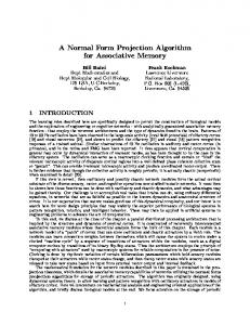
The following example illustrates the ability of the SCTAP model to produce more realistic assignment results compared to standard traffic assignment. Consider the network presented in Figure 1Figure1, which consists of a central intersection that may represent a city center surrounded by two ring roads. Travel times on each link are given by the BPR formula with parameters α = 0.15 and β = 4 . The free-flow travel times ( t0 ) and capacities of the links in this network are presented inTable 1. Trip demands are for passing traffic (1→2, 2→1) and for trips to the center (1→7, 2→7). These demands are presented inTable 2. 9
10
3
6
1
7
2
4
5
8
11
Figure1. Example network
User equilibrium flows on this network were found using two models: the standard model and the side-constrained model. In the latter, constraints on intersection flows, given by Equation Fout! Verwijzingsbron niet gevonden., were imposed on intersections 3, 4, 5 and 6. Both solutions are presented in Figure 2. The unconstrained solution shows high levels of traffic passing through the center and the inner ring. The outer ring is not used at all. As a result the flows on four links exceed capacities. The flows through intersections 3, 4, 5 and 6 are more than double the capacity of these intersections. It is more realistic to assume that limited capacities and delays near the center will divert traffic to other paths bypassing the center. This is apparent in the SCTAP solution: only center-bounded traffic goes into the center. Passing traffic is diverted from the center to the two ring roads. The resulting link
184
A radient Projection Algorithm for Side-constrained Traffic Assignment
flows are such that the flows through all intersections satisfy the capacity constraints of these facilities. This example shows that the introduction of side-constraints can significantly alter traffic assignment patterns and provide more realistic and plausible predictions. The impact on decision making may not only be in terms of the conclusions that will be drown from the assignment results, but also in terms of the fidelity decision-makers associate with the assignment results. Table 1. Link parameters Up Node 1 1 1 1 2 2 2 2 3 3 3 3 4 4 4 4 5 5 5 5
Down Node 3 4 8 9 5 6 10 11 1 6 7 9 1 5 7 8 2 4 7 11
t0
C
20 20 30 30 20 20 30 30 20 15 6 20 20 15 6 20 20 15 6 20
3000 3000 4000 4000 3000 3000 4000 4000 3000 3000 2000 4000 3000 3000 2000 4000 3000 3000 2000 4000
Table 1 Trip demands Origin 1 1 2 2
Destination 2 7 1 7
Demand 4000 3000 4000 3000
Up Node 6 6 6 6 7 7 7 7 8 8 8 9 9 9 10 10 10 11 11 11
Down Node 2 3 7 10 3 4 5 6 1 4 11 1 3 10 2 6 9 2 5 8
t0
C
20 15 6 20 6 6 6 6 30 20 30 30 20 30 30 20 30 30 20 30
3000 3000 2000 4000 2000 2000 2000 2000 4000 4000 4000 4000 4000 4000 4000 4000 4000 4000 4000 4000
Joseph N. Prashker and Tomer Toledo
820
2000
185
3500
820 2680 1180 3500
2680
2000
1180
1180
2000
2680
3500
1180 2680 820 2000
3500
820
UE not considering constraints
1250 1250
1250
1250 1250
750
1250
2250
750
750 1500 750
1500
2250
2250
750
1500
2250 1250
1500 750
750
750
1250
1250
1250
1250 1250 UE considering constraints Legend V/C