Proceedings of the 15th International Conference on Auditory Display, Copenhagen, Denmark May 18 - 22, 2009
A GRAPH-BASED SYSTEM FOR THE DYNAMIC GENERATION OF SOUNDSCAPES Andrea Valle, Vincenzo Lombardo, Mattia Schirosa CIRMA-Universit`a di Torino via Sant’Ottavio 20, 10124, Torino, Italy
[email protected],
[email protected],
[email protected] ABSTRACT
atmosphere [18]. At the same time, musique concr`ete has prompted composers to think about sounds as sound objects. During the ’60-’70s many composers started working with sound field recording. Sharing the musique concr`ete attitude towards sound, they have been strongly influenced by the soundscape studies. Not by chance, many of Murray Schafer’s associates were composers. Thus, the concept is widely present in many contemporary musical forms, as the soundscape itself is regarded as a form of “natural” music composition (in general, cf. [19]). More, “soundscape composition” identifies a mainly electro-acoustic genre, starting from natural acoustic environmental sounds, sometimes juxtaposed with musical scores. Also, sound designers working for cinema and TV have contributed to the diffusion of the term, indicating with “soundscape” the idea of an acoustic scenario to be added/adapted to the moving image ([20], cf. [21]).
This paper presents a graph-based system for the dynamic generation of soundscapes and its implementation in an application that allows for an interactive, real-time exploration of the resulting soundscapes. The application can be used alone, as a pure sonic exploration device, but it can also be integrated into a virtual reality engine. In this way, the soundcape can be acoustically integrate in the exploration of an architectonic/urbanistic landscape. The paper is organized as follows: after taking into account the literature relative to soundscape, a formal definition of the concept is given; then, a model is introduced; finally, a software application is described together with a case-study. 1. INTRODUCTION The term “soundscape” has been firstly introduced (or at least, theoretically discussed) by R. Murray Schafer in his famous book The tuning of the world [1]. Murray Schafer has lead the research of the World Forum For Acoustic Ecology, a group of researchers and composers who empirically investigated for the first time the “environment of sounds” in different locations both in America and in Europe. Murray Schafer and his associates studied for the first time the relation between sounds, environments and cultures. Hence on, the diffusion of the term has continuously increased, and currently the concept of soundscape plays a pivotal role at the crossing of many sound-related fields, ranging from multimedia [2] to psychoacoustics [3], from job environment studies [4] to urban planning [5], from game design [6] [7], to virtual reality [8], from data sonification [9] to ubiquitous computing [10] [11]: in particular it is a fundamental notion for acoustic design [12] [13], electroacoustic composition [14], auditory display studies ([15]). Indeed, it can be noted that such a diffusion of the term is directly proportional to the fuzziness of its semantic spectrum. It is possible to individuate three main meanings of the term “soundscape”, related to three different areas of research: • Ecology/anthropology [16]. Since Murray Schafer’s pioneering work, this perspective aims at defining the relevance of sound for the different cultures and societies in relation to the specific environment they inhabit. A soundscape is here investigated through an accurate social and anthropological analysis. The goals are two. On the one side, the researchers are interested in documenting and archiving sound materials related to a specific socio-cultural and historical context. On the other side, they aim at leading the design of future projects related to the environmental sound dimension. • Music and sound design [17]. The musical domain is particularly relevant. All along the 20th century, ethnomusicological studies, bruitism, “musique d’ameublement” and “musique anecdotique” have fed the reflection on environmental sound dimension as acoustic scenery or as scenic
• Architecture/urban planning [22]. In recent years, electroacoustic technology and architectural acoustics have allowed to think about the relation between sound and space in a new form, in order to make citizens aware of the sonic environment (the soundscape) they live in, so that they can actively contribute to its re-design. Many architectural projects have been developed descending from these assumptions [23]. The concept of “lutherie urbaine” has been proposed as a combined design –of architecture and of materials– for the production of monumental components located in public spaces and capable of acting like resonators for the surrounding sound environment [24]. It must be noted that such a complex and rich set of features related to soundscape is extremely relevant because it demonstrates that the problem of the relation between sound and space cannot be solved only in acoustic or psycho-acoustic terms. An acoustic or psycho-acoustic approach considers the relation among sound, space and listener in terms of signal transfer [25]. Acoustic ecology, through a large body of studies dedicated to soundscape description and analysis ([1], has pointed out that the perception of soundscape implies the integration of low-level psychoacoustic cues with higher level perceptual cues from the environment, its cultural and anthropological rooting, its deep relations with human practices. The integration of soundscape in a landscape documentation/simulation is crucial in order to ensure a believable experience in human-computer interaction [26]. A consequence of the integration among different perceptual domains and among multilevel information is that the study of soundscape requires to include phenomenological and semiotic elements. In this sense, the study of soundscape can benefit from the research in “audiovision”, i.e. the study of the relation between audio and video in audiovisual texts (film, video etc) [27]. More, soundscape studies have highlighted the relevance of different listening strategies in the perception of the sonic environments: from a phenomenological perspective ([28], [29]) it is possible to identify an “index-
ICAD09-1
Proceedings of the 15th International Conference on Auditory Display, Copenhagen, Denmark May 18 - 22, 2009
ical” listening (when sounds are brought back to their source), a “symbolic” listening (which maps a sound to its culturally-specific meanings), an “iconic” listening (indicating the capabilites of creating new meanings from a certain sound material [28]). 2. FOR A DEFINITION OF SOUNDSCAPE As the semantic spectrum of the term “soundscape” is quite fuzzy, a modelization of soundscape requires firstly of all to provide an explicit definition. With this aim, we need to introduce other concepts. A “sound object” is a cognitive and phenomenological unit of auditory perception [28]. It can be thought as an “auditory event” [30] and integrated in terms of ecological and cognitive plausibility in the auditory scene analysis approach [31]. Its nature of “object” is intended to emphasize its semiotic quality. This means that a sound object is always related to a specific listening practice, so it is not exclusively placed at the perceptual level but is also related to a specific cultural context. As sound objects are temporal objects, their description must include a temporal organization. Traditionally, the soundscape studies have insisted on a tripartite typology of sounds in relation to their socio-cultural function [16]: keynote sounds, signal sounds, soundmarks. Keynote sounds are the sounds heard by a particular society continuously, or frequently enough, to form a background against which other sounds are perceived (e.g. the sound of the sea for a maritime community). Signals stands to keynotes sounds as a figure stands to a background: they emerges as isolated sounds against a keynote background (e.g. a fire alarm). Soundmarks are historically relevant signals (e.g. the ringing of the historical bell tower of a city). While this classification is intended as a guidance for the analysis of the soundscape in its cultural context, here we propose a different classification focusing on the perceptual and indexical properties of the soundscape. In particular, the sound objects of a soundscape can be distinguished in: • atmospheres: in relation to sound, B¨ohme has proposed an aesthetics of atmospheres [32]. Every soundscape has indeed a specific “scenic atmosphere”, which includes explicitly an emotional and cultural dimension. An atmosphere is an overall layer of sound, which cannot be analytically decomposed in single sound objects, as no particular sound object emerges. Atmosphere characterizes quiet states without relevant sound events. While keynote sounds are intended as background sounds (i.e. they are a layer of the soundscape), atmospheres identify the whole sound complex. • events: an event is a single sound object of well-defined boundaries appearing as an isolated figure. In this sense, it is similar to a signal as defined in soundscape studies. • sound subjects: a sound subject represents the behavior of a complex source in terms of sequencing relations between events. In other words, a sound subject is a description of a sound source in terms of a set of events and of a set of sequencing rules. In other words, an atmosphere is a sound object which source cannot be identified, as the source coincides with the whole environment. Events and sound subjects are sound objects related to specific sources. In the case of an event, the behavior of the source is simple, and can be thought as the emission of a specific sound object. In case of a sound subject, the behavior is complex and must be specified as a set of generation rules. Still, the previous classification of sound objects is not enough to exhaustively define a soundscape. A soundscape is not only
a specific structure of sound objects arranged in time (otherwise, every piece of music could be defined a soundscape), but it is related to a space, so that the exploration of such a space would reveal other nuances of the same soundscape. This exploration is performed by a listener, not to be intended as a generic psychoacoustic subject but considered as a culturally-specific one: through the exploration of the space, the listener defines a transformation on the sound objects that depends on the mutual relation between her/himself and the objects. The transformation is operated by the listener and is intended as a global response of the environment to her/his exploration. The transformation is both spatial –as it depends on features related to the listening space (e.g. reverberation)– and semiotic –as it depends on cultural aspects (e.g. specific listening strategies). By coupling the spatial and semiotic aspects, Wishart [33] has discussed in depth the symbolic construction of landscape in acousmatic listening conditions, by taking into account this overall sound dimension. For Wishart “the landscape of a sound-image” is “the imagined source of the perceived sounds” ([33]: p. 44). In this sense, for Wishart the landscape of the sounds heard at an orchestral concert is musician-playing-instruments, exactly as the landscape of the same concert heard over loudspeakers through recording is also musician-playing-instruments. The reconstructed landscape is a semiotic construction based on cultural coding of soundscape. Wishart proposes a semiotic/phenomenological description of natural soundscapes. For instance: moorlands reveal a lack of echo or reverberation, sense of great distance, indicated by sounds of very low amplitude with loss of high-frequency components; valleys display a lack of distance cues and possibly include some specific image echos; forests are typified by increasing reverberation as the distance of the source from the listener increases ([33]: p. 45). Such a characterization can be semantically described through three continuous parameters: dynamics (cf. in music: from ppp to fff ), reverberation (expressed along the axis dry/wet), brightness (in timbral studies, typically along the axis bright/dull). It can be noted that a similar semantic description is strictly correlated to psychoacoustic cues, respectively intensity, direct-to-reverberant ratio, spectrum [26]. These three categories provide three descriptive axes for a qualitative evaluation of the global acoustic behavior of the soundscape: each soundscape can then be represented as a point in a three dimensional, qualitative space. From the previous discussion, we can provide the following definition: A soundscape is a temporal and typological organization of sound objects, related to a certain geo-cultural context, in relation to which a listener can apply a spatial and semiotic transformation. 3. TOWARDS A FORMALIZED MODEL It is worth noting that, despite the profusion of usages, there are neither models nor applications aiming at a simulation of a soundscape starting from the analysis of an existing soundscape. Listen [34] works on the generation and control of interactive soundscapes, but does not include an explicit modelization of the soundscape itself. Tapestrea [17] is designed to generate “environmental audio” in real time, but does not define any relation between sound and space. In devising a computational model to be implemented in an application, a first issue concerns the relation between the acoustic and the phenomenological level. As a computer deals only with sound signals, for each sound object a matching signal must be individuated [26]. The problem is particularly relevant when the sound objects are simultaneous. The more complex a soundscape is, the more difficult is to unambiguously identify a signal corresponding to a sound object. Hence on, a “sound material” will be an audio signal corresponding to a certain sound object. Thus, in
ICAD09-2
Proceedings of the 15th International Conference on Auditory Display, Copenhagen, Denmark May 18 - 22, 2009
the analysis of a complex soundscape, there are at least two difficult issues: first, the decomposition of the sound continuum into sound objects; second, the retrieval of the corresponding signal for each sound object. As an example, in the soundscape of a restaurant kitchen, the decomposition of the overall sound into unitary elements can be quite vague, as some elements are easy recognizable (creaking fire, falling water, voices of the cooks), but on the other side there is a diffuse texture made of a large amount of microsonic events that can be hardly brought back to their sources. But even after having identified the sound objects, it can be very difficult to extract isolated signals from the global soundscape. The first issue can be identified as “semiotic discretization”, the second as “acoustic discretization”: it is thus possible to consider both a semiotic discretization error (Sde) and an acoustic discretization error (Ade). If the space is taken into account while defining a soundscape (i.e. a soundscape is indexically related to a certain space), it can happen that a space presents different sound regions. “Soundscape” will then indicate the summation of all the sound regions that a listener will be able to explore. Such regions can be called “zones”. A zone is a sound region that can include all the different kinds of sound objects previously discussed: atmospheres, events and sound subjects. In turn, a sound subject SS represents the behavior of a source in term of sequencing relations on a set of sound objects. It can be then defined as the summation of all the composing events and their spatial and temporal relations: X SS = E+R A zone is then the summation of all the atmospheres A, the events E, and the sound subjects SS, plus the set of temporal and spatial relations R defined over them. As a consequence, a zone Z can be formally defined as follows: X Z= (A + E + SS) + R Typically, in the literature a soundscape is considered a unitary object characterized by a set of relevant features. A “static” soundscape SSC (see later for static/dynamic opposition) is the summation of all the different sound zones Z, without the errors induced by semiotic and acoustic quantization (Sde and Ade). Hence the following definition: X SSC = ( Z) − Sde − Ade As noted, the previous definition is still static, as it does not take into account the role of the listener. The given definition considers all the sound objects, but still does not recognize a role for the listener: in this sense is still static. As already discussed, the presence of a listener –exploring the space– allows to reveal the global acoustic properties of the space itself. The definition of a “dynamic” soundscape DSC considers the listener L as a function receiving as argument a static soundscape SSC, intended as a collection of sound objects and their relations. DSC = L(SSC) Starting from the previous definition of soundscape, it is possible to propose a model for the simulation of soundscapes. The proposed system is named GeoGraphy and features four phases (Fig. 1): 1. classification, analysis and recording, 2. production, 3. generation, 4. evaluation. 4. CLASSIFICATION, ANALYSIS AND RECORDING The first phase aims at gathering data from the real environment. It includes the classification of sound objects, their perceptual analysis and the recording of the related sound material.
First, general information on the space are collected, including cultural features (e.g. if it is a religious or a secular space) ascribed to it, topographical organization (e.g. if it contains pedestrian areas), global acoustic properties (e.g. if it is reverberant or not and how much). Then, we proceed at the identification of sound objects. This is a particularly delicate task, as it cannot make use of measurements but must rely on qualitative parameters. In order to limit the subjectivity of evaluation and to reduce the complexity and arbitrariness of the whole operation, a specific two-step procedure has been devised. The first step focuses on an “absentminded” exploration of the soundscape: the analyst must be perceptually open, adhering to a passive listening strategy [21]. In this way it becomes possible to identify the most relevant sound objects of the overall soundscape, i.e. the ones that are evident even to the least aware listeners. Moreover, the analyst carries out interviews with different kinds of listeners, dealing with their global experience of the soundscape at different levels (perceptual, emotional, cultural). In the second step, an active listening strategy locates the sound objects in the space. The soundscape is investigated in depth, so that now even less prominent sound objects can be detected and analyzed. The step consists in an on-site exploration, so that the eye can complement and help the ear in the retrieval process while aiming at identifying areas with homogeneous sound objects. As an example, in case of a market, different areas can be identified in relation to different stands, pedestrian crossovers, loading/unloading areas, parking zones. It is thus possible to create a sound map (Fig. 7) partitioned into areas with sound objects assignment. Then, we focuses on the analysis of specific sequences of sound objects. As an example, loading/unloading procedures in a market are characterized by specific sequences of sounds: it can be said that they show a specific syntax, i.e. temporal ordering. The analysis of the temporal behavior of the syntactical properties of sound objects is fundamental for the parameterization of the generative algorithm (see later). Finally, recordings of raw audio material from the environment are realized. The recording process tries to avoid information loss. In fact, if a sound material is not recorded, it cannot be recovered any more in the next phases of the process. As a consequence, the recording procedure is based on a double approach. On one side, large portions of soundscape are recorded via an omnidirectional microphone: so, a large quantity of raw material is available for editing and processing. On the other side, high directivity microphones (“shotgun”) are used to capture a wide variety of emissions while minimizing undesired background. This collection of sound emissions can be filtered out in the analysis step. The data gathered in this phase are furtherly refined in the production phase. 5. PRODUCTION The production phase focuses on the creation of the soundscape database. The database is intended as a catalogue of the soundscape information and contains all the previously discussed information. The fundamental operation in this phase is the creation of sound materials. As discussed, a sound material is the audio signal associated with a sound object. The phase consists of two steps. First, recordings are analyzed through an acousmatic listening while the classification/recording phase relies on symbolic and indexical listening, trying to identify culturally relevant objects and locate them in the space. The production phase focuses on iconic listening strategy, since it considers the sounds as perceptual objects, regardless of their meaning or relation to the environment. After an accurate, acousmatic listening, the final set of sound ob-
ICAD09-3
Proceedings of the 15th International Conference on Auditory Display, Copenhagen, Denmark May 18 - 22, 2009
Soundscape Analysis of sound objects
Recording
Simulated soundscape
Soud objects/ structures
User Interactive exploration . GeoGraphy . Sound Interpreter . Libraries
Sound materials Annotated sound material database
Spatial and behavioral information
Resynthesis
Evaluation tests
4. Evaluation 1. Classification/Analysis/ Recording
2. Production 3. Generation
Figure 1: The GeoGraphy model. The generated soundscape (right) contains a reduced set of relevant sound objects.
jects is identified. Then, sound materials are created: this operation involves some editing on audio samples (e.g. noise reduction, dynamics compression, normalization). In case different sound objects reveal analogous phenomenological features, they can be grouped into a single sound material. For example, the sounds of forks, spoons and knifes are indexically different; at an iconic listening, they can reveal a substantial phenomenological identity, so that they are realized through the same sound material. The second step is a general reviewing phase of the previous information in order to create a final sound map. If some sound material is lacking, a new recording session is planned, targeted to that specific sound object. In this way a feedback loop is defined from production to classification (hence the double arrow in Fig. 1). 6. GENERATION The information retrieved from the annotation/analysis of the real soundscape is then used to generate a synthesized soundscape. The generation process involves two components. The first is a formal model defining a dynamic algorithm for the sequencing of the sound objects. In order to be dynamic, the algorithm must meet two requirements. First, it must be generative, i.e. to be able to create an infinite set of sequences of sound objects. This sequence represents a continuous variation over the same soundscape from a finite set of sound objects. Second, the algorithm must be able to merge the information coming from the sequencing process with the user’s navigation data. In this way, a soundscape can be simulated and explored interactively. The generative model is based on graphs and extends the GeoGraphy system [35] [36]. The second component is responsible for the interpretation of the data generated by the model in a sonic context. Hence, it is named “Sound Interpreter”. In the following subsections we first describe the two levels of GeoGraphy, and then the Sound Interpreter. 6.1. GeoGraphy, I level: graphs Graphs have proven to be powerful structure to describe musical structures ([37]): they have been widely used to model sequencing relation over musical elements belonging to a finite set. It can be disputed if non-hierarchical systems are apt for music organization, as hierarchical structures have proven to be useful in modeling e.g. tonal music ([38]). But hierarchical structures are not present in soundscapes: on the contrary, it is common to consider soundscape in terms of multiple parallel and independent layers
vLab woodLow A
A: woodLow
woodHi B
vID 3: 0.5
woodHi woodLow woodHi B A B
1: 0.7 eID: eDur
4: 1.0 B: woodHi 2: 1.2
4: 1.0
2: 1.2
1: 0.7
3: 0.5
vDur (0.7)
Figure 2: A graph (left) and a resulting sequence (right). A and B: vertices; 1,2,3: edges. The duration of the vertices is 0.7.
of sound ([1]). A common feature of all these graph representations devised for music is that they generally do not model temporal information: the GeoGraphy model relies on time-stamped sequences of sound objects. The sequencing model is a direct graph (Figure 2), where each vertex represents a sound object and each edge represents a possible sequencing relation on pairs of sound objects. This graph is actually a multigraph, as it is possible to have more than one edge between two vertices; it can also include loops (see Figure 2 on vertex 2). Each vertex is labeled with the sound object duration and each edge with the temporal distance between the onsets of the two sound objects connected by the edge itself. The graph defines all the possible sequencing relation between adjacent vertices. A sequence of sound objects is achieved through the insertion of dynamic elements, called “graph actants”. A graph actant is initially associated with a vertex (that becomes the origin of a path); then the actant navigates the graph by following the directed edges according to some probability distribution. Each vertex emits a sound object at the passage of a graph actant. Multiple independent graph actants can navigate a graph structure at the same time, thus producing more than one sequence. In case a graph contains loops, sequences can also be infinite. As modeled by the graph, the sound object’s duration and the delay of attack time are independent: as a consequence, it is possible that sound objects are superposed. This happens when the vertex label is longer than the chosen edge label. A soundscape is a set of sequences, which are superposed like tracks: in a soundscape there are as many sequences as graph actants. At the first level the generation process can be summarized as follows. Graph actants circulates on the graph: there are as many simultaneous sound object sequences as active graph actants. In the generation process, when an actant reaches a vertex, it passes to the level II the vertex identifier: the ID will be used in the map of graphs to determine if the vertex itself is heard by the Listener (see later). An example is provided in Figure 2. The graph (left) is defined by two ver-
ICAD09-4
t
Proceedings of the 15th International Conference on Auditory Display, Copenhagen, Denmark May 18 - 22, 2009
tices and four edges. The duration of both vertices is set to 0.7 seconds. In Figure 2 (right), vertices are labeled with an identifier (“1”, “2”). More, each vertex is given a string as an optional information (“woodLow”, “woodHigh”), to be used in sound synthesis (see later). A soundscape starts when an actant begins to navigate the graph, thus generating a sequence. Figure 2 (left) represents a sequence obtained by inserting a graph actant on vertex 1. The actant activates vertex 1 (“woodLow”), then travels along edge 4 and after 1 second reaches vertex 2 (“woodHi”), activates it, chooses randomly the edge 2, re-activates vertex 2 after 1.2 seconds (edge 2 is a loop), then chooses edges 1, and so on. While going from vertex 1 to vertex 2 by edge 3, vertex duration (0.7) is greater then edge duration (0.5) and sound objects overlap. The study of the temporal pattern of the many sound objects provides the information to create graphs capable of representing the pattern. Every graph represents a certain structure of sound objects and its behavior. Different topologies allow to describe structure of different degrees of complexity. This is apparent in relation to the three types of sound objects previously introduced. Atmosphere are long, continuous textural sounds: they can be represented by a single vertex with an edge loop, where the vertex duration (typically of many seconds) coincides with the edge duration (Figure 3, a). In this sense, atmospheres simply repeat themselves. Analogously, events can be represented by graphs made of a single vertex with many different looping edges, which durations are considerably larger than the duration of the vertex (Figure 3, b). In this way, isolated, irregularly appearing events can be generated. Indeed, the graph formalism is mostly useful for sound subjects. A complex, irregular pattern involving many sound objects can be aptly described by a complex multigraph (Figure 3, c). The multigraph can generate different sequences from the same set of sound objects: in this sense, it represents a grammar of the sound subject’s behavior.
graph
energetic areas
distance displacement angle
active vertex audibility area Listener
trajectory
Figure 4: Listener in the map of graphs. The audibility radius filters out active vertices falling outside.
control; the audibility area defines the perceptual boundaries of the Listener. The Listener can be thought as a function that filters and parameterizes the sequences of sound objects generated by the graph actants. Every time a vertex is activated by a graph actant, the algorithm calculates the position of the Listener. If the intersection between the Listener’s audibility area and the vertex’s energetic area is not void, then the Listener’s orientation and distance from the vertex are calculated, and all the data (active vertex, position, distance and orientation of the Listener) are passed to the DSP module. In sum, the level II receives a vertex ID from the level I, and adds the information related to its mutual position with respect to the Listener: distance and displacement along the two planes. The two-level system outputs a sequence of time-stamped vertex IDs (I level) with positional information added (II level). Actually, the level II models the space as a 2-dimensional extension, and assumes that the sound sources (represented by vertices) are static. 6.3. The Sound Interpreter
a
b
c
Figure 3: Possible topologies for atmosphere, events and sound subjects (sizes of vertices and edge lengths roughly represents durations).
6.2. GeoGraphy, II level: map of graphs At the second level, the vertices are given an explicit position in terms of coordinates of a Euclidean 2-dimensional space (hence the name GeoGraphy: graphs in a space): in this way, the original location of a sound object is represented. Each vertex is given a radiation area: the radius indicates the maximum distance at which the associated sound object can be heard. The space is named map of graphs. A map contains a finite number of graphs (n), which work independently, thus generating a sequences, where a is the total number of the graph actants that navigate in all the graphs. As there is at least one graph actant for each graph, there will be a minimum of n tracks (a ≥ n), i.e. potential layers of the soundscape. This second metric level allows to include the exploration process. Inside the map of graphs, a dynamic element, a “Listener” determines the actually heard soundscape. The Listener is identified by a position, an orientation and an audibility area (see Fig. 4). The position is expressed as a point in the map; the orientation as the value in radiant depending on the user’s interaction
The GeoGraphy model does not make any assumption about sound objects, whose generation is demanded to an external component. It defines a mechanism to generate sequences of referred sound objects (grouped in sequences). During the generation step, the data from the model are passed to the Sound Interpreter. As discussed, for each event the data include attributes of space and sources, and movement. The Interpreter defines the audio semantics of the data by relating them to transform functions. These transform functions are grouped into libraries containing all the necessary algorithms to generate the audio signal: they define a mapping schema associating the vertex IDs to sound materials in the database, and spatially-related data to audio DSP components, e.g. relating distance to reverberation or displacement to multi-channel delivery. By using different libraries the system allows to define flexible mapping strategies. As an example, one can consider a “cartoonification” library. Rocchesso and his associates [26] have proposed cartoonification techniques for sound design, i.e. simplified models for the creation of sounds related to physical processes (e.g. bouncing, cracking, water pouring etc). The cartoonification process starts from an analysis of the physical situation and simplifies it, retaining only the perceptual and culturally relevant features. Cartoonification is particularly relevant for GeoGraphy as our approach is not intended as a physical modelization, but as a semiotic/phenomenologic reconstruction. In fact, the map of graphs in itself can be considered as a cartoonification of the real space. A cartoonification library can use the distance parameter as a general controller for audio processing: distance can be used to calculate amplitude scaling, reverberation parameters and lowpass filter coefficients, i.e. the greater the distance, the lower the amplitude
ICAD09-5
Proceedings of the 15th International Conference on Auditory Display, Copenhagen, Denmark May 18 - 22, 2009
Libraries
Database I - emit vertices
Graphs
II - add Listenrelated params Map of graphs
GeoGraphy
...
be connected to a virtual reality engine, in order to allow an audiovisual integration of an architectonic-urbanistic space.
- audio processing and delivery
ˆ 9. CASE-STUDY: THE MARKET OF THE “BALON”
Sound Interpr eter
The model has been tested on a simulation of the soundscape of the Balˆon, Turin’s historical market (see [40]). The market is a
- maps data to sound libraries
Figure 5: The generation process. In this case the final delivery is stereo. multiplier, the higher the reverberation value, the lower the lowpass filter’s cut frequency. Orientation will typically be used to calculate panning. In this way, it is possible to create “sound symbols” of the whole landscape by providing global, semiotically recognizable, perceptual cues. In this sense, sound symbols can be thought as cartoonified models of the global, physical properties of the space. Other libraries can include “fictional” rendering of the soundspace, e.g. where the distance is directly proportional to the cut frequency of the lowpass filter, thus inverting the cartonified schema. In this way, the continuous nature of the space (populated by the same sound objects) is preserved, even if the global result can sound “alien”. Alien mappings are useful to create artificial spaces (for artistic purposes, from music to sound design) and to test the degree of soundscape invariance over different space models. 7. EVALUATION The resulting simulation is evaluated through listening tests, taking into account both the sound materials and the transformations induced by space. As the competences about sound can vary dramatically from a user to another, the evaluation procedure considers four different typologies of listeners: occasional visitors, regular goers, non-sensitized listeners, sensitized listeners (musician/sound designers). Throughout evaluation tests are still to be carried out. We plan to evaluate the quality of the simulated soundscape by comparing it with a real one. In particular, we will define a path in a real space and record the resulting soundscape with a stereo microphone while going through it. Then we will simulate in GeoGraphy the same soundscape following the procedure described above: the Listener’s trajectory will reproduce the real exploring path. In this way, it will be possible to compare the simulation with the original recording over different listeners, thus evaluating its global effectiveness. 8. IMPLEMENTATION The GeoGraphy system has been implemented in the audio programming language SuperCollider ([39], see Fig. 6), which features a high-level, object-oriented, interactive language together with a real-time, efficient audio server. The SuperCollider language summarizes aspects that are common to other general and audio-specific programming languages (e.g. respectively Smalltalk and Csound), but at the same time allows to generate programmatically complex GUIs. The application includes both graphical user interfaces and scripting capabilities (see Fig. 6). Graph structures are described textually (with a dot language formalism) and displayed graphically. Both the activation of vertices and the interactive exploration process can be visualized in real time. The Open Sound Control (OSC) interface, natively implemented in SuperCollider, allows for a seamless network integration with other applications. As a typical example, the GeoGraphy application can
Figure 7: Map of a portion of the Balˆon market: numbers and names indicate sound zones identified during the annotation phase. typical case of a socio-cultural relevant soundscape. In particular, the market of the Balˆon has a long tradition (it has been established more than 150 years ago): it is the greatest outdoor market in Europe and represents the commercial expression of the cultural heritage of the city of Turin. During the century, it has tenaciously retained its identity, characterized by the obstinate will of the workers of sharing its government’s responsibility. It is probably the part of Turin where the largest number of different social realities and cultures inhabit. As a consequence, its soundscape manifests an impressive acoustic richness. First, it includes languages and dialects from all the regions of Italy, South America, Eastern Europe, North Africa. More, there are many qualitatively different sound sources: every day the market serves 20,000 persons (80,000 on Saturday), and 5,000 persons work there every day. The analysis of the case-study initially focused on the sociocultural dimension of the market, and on short informal interviews to local workers, customers and worker representatives. The interviews occurred while performing the first absentminded explorations of the place, and annotating the most common sound objects: the sound of plastic shoppers (noticed like a keynote sound), the shouts of the merchants, the pervasive noises of vehicles. Then, sound signals concern specific market stands. This phase has lead to the creation of a sound map where specific areas have emerged. As an example, fruit stands include the sound of hard fruits being knocked over the iron tables or of fresh fruit moved over the table’s surface. The stands of the anchovy sellers have proven to be very different, including sounds of metal cans, anchovies being beaten over wood plates, olives thrown in oil. Subsequently, geographical-sound zones have been created: the analysis of the soundscape has led to define five indipendent zones formed by characteristic elements (events and sound subjects that have a par-
ICAD09-6
Proceedings of the 15th International Conference on Auditory Display, Copenhagen, Denmark May 18 - 22, 2009
Actant Control Window
Map of Graphs GUI
SuperCollider Control Window
SupeCollider Server Window
Figure 6: A screenshot from the application with a graph width edge/vertex durations (background), the Actant Control Window and other SuperCollider-related GUIs for real-time control.
ticular presence in a zone, and that do not often appear in another). It was been possible to define specific atmospheres. In Fig. 7 all the zones are illustrated with an identifying index. Zone 5 presents only vegetable and fruit stands: in this sense, it is a “pure” example of sounds related to human activity, as there are no other sound objects (related, e.g., to motor vehicles). Zone 4 is formed by different and sparse stands; it presents a less prominent density of market activity sounds because the passage area is bigger, and the sound of the customers is louder. Zone 3 shows a mixup of sounds related to market and street/parking areas. Zone 2 is filled by the sounds of people in the street passage, with trams and buses. Zone 1 refers to the sound atmosphere made up of sounds from delivery trucks, hand-carts and gathering of packing boxes from stands. The best field recordings have been chosen in order to create the sound materials related to each sound object. Typically, many different sound materials related to the same sound object have been stored, so that the complexity of the original soundscape would not be lost. The phase has included an in-depth analysis of the sound object’s behavior and the positioning of the sound objects over the sound map. Graphs have proven to be capable of expressing very different behaviours. As an example, the butcher’s knife beating the meat generates a single sound object repeated with a specific pattern, which can be expressed by a graph made of a single vertex with a looping edge. Payment procedures have revealed a chain of many different sound objects: there is a specific pattern of sound objects, involving the rustle of the wrapping paper and the shopper, the tinkling of coins, the different noises of the cash register marking the many phases of the action. In this case, a much more complex graph is needed. Finally, acousmatic listening of the recordings has allowed to identify a large quantity of unexpected sound objects. In some cases, this has lead to the realization of other recording sessions in the market. The information gathered during the annotation process has been used to simulate the Balˆon’s soundscape through the GeoGraphy application. The evaluation phase is actually in a preliminary phase, but has included both experts (sound designers, soundscape researchers) and occasional listeners, with positive results in both cases. Reportedly, a prominent feature lies in the generative nature of the system: even if based on a discrete set of sound materials, the use of graph-based sequencing avoids the feeling of artificiality typical of sound sample looping, as the soundscape is in continuous transformation.
10. CONCLUSIONS AND FUTURE WORK The notion of soundscape is increasingly relevant not only in contemporary culture, but also in the world of sound-related studies. Still, a rigorous definition of the concept is lacking. By providing such a formal definition, it is possible to propose a generative model for the simulation of not only real soundscapes. GeoGraphy provides a theoretical framework for the modelling of soundscape in terms of both temporal information describing sound time patterns (via the vertex/edge labeling) and spatial information encoding the site/observer relation (via vertex positioning). The Sound Interpreter allows to create different soundscapes form the same set of sound objects by defining specific mapping strategies to different libraries. GeoGraphy implementation in SuperCollider can operate interactively in real time and it can be integrated in other multimedia applications. A major issue in GeoGraphy concerns the generation of multigraphs, actually to be carried out manually and potentially quite time-consuming. We are planning to extend the system so to include the automatic generation of graphs starting from information stored in the database or from sound-related semantic repertoires (see [41]). The database itself can eventually include not only sound materials created from direct recording but also samples from available sound libraries. An interesting perspective is to investigate user-generated, online databases such as Freesound1 : in this case, the graph generation process can be governed by social tagging. 11. REFERENCES [1] R. Murray Schafer, The Tuning of the World, McClelland & Steward and Knopf, Toronto and New York, 1977. [2] Matthew Burtner, “Ecoacoustic and shamanic technologies for multimedia composition and performance,” Organised Sound, vol. 10, no. 1, pp. 3–19, 2005. [3] Federico Fontana, Davide Rocchesso, and Laura Ottaviani, “A structural approach to distance rendering in personal auditory displays,” in Proceedings of the International Conference on Multimodal Interfaces (ICMI 2002), Pittsburgh, PA, 2002.
ICAD09-7
1 http://www.freesound.org/
Proceedings of the 15th International Conference on Auditory Display, Copenhagen, Denmark May 18 - 22, 2009
[4] Iain McGregor, Alison Crerar, David Benyon, and Catriona Macaulay, “Sounfields and soundscapes: Reifying auditory communities,” in Proceedings of the 2002 International Conference on Auditory Display, Kyoto, 2002. [5] Benjamin U. Rubin, “Audible information design in the New York City subway system: A case study,” in Proceedings of the International Conference on Auditory Display ’99, Glasgow, 1998. [6] Milena Droumeva and Ron Wakkary, “The role of participatory workshops in investigating narrative and sound ecologies in the design of an ambient intelligence audio display,” in Proceedings of the 12 th International Conference on Auditory Display, London, 2006. [7] Johnny Friberg and Dan G¨ardenfors, “Audio games: New perspectives on game audio,” in Proceedings of the 2004 ACM SIGCHI International Conference on Advances in computer entertainment technology, New York, 2004, pp. 148– 154, ACM Press. [8] Stefania Serafin, “Sound design to enhance presence in photorealistic virtual reality,” in Proceedings of the 2004 International Conference on Auditory Display, Sydney, 2004. [9] T. Hermann, P. Meinicke, and H. Ritter, “Principal curve sonification,” in Proceedings of International Conference on Auditory Display, 2000, 2000. [10] Andreas Butz and Ralf Jung, “Seamless user notification in ambient soundscapes,” in IUI ’05: Proceedings of the 10th international conference on Intelligent user interfaces, New York, NY, 2005, ACM Press. [11] Fredrik Kilander and Peter L¨onnqvist, “A whisper in the woods - an ambient soundscape for peripheral awareness of remote processes,” in Proceedings of the 2002 International Conference on Auditory Display, Tokyo, 2002. [12] VV.AA., “The tech issue ...to be continued,” Soundscape, vol. 3, no. 1, July 2002. [13] VV.AA., “Acoustic design,” Soundscape, vol. 5, no. 1, 2004. [14] Hildegard Westerkamp, “Linking soundscape composition and acoustic ecology,” Organised Sound, vol. 7, no. 1, 2002. [15] Bradley S. Mauney and Bruce N. Walker, “Designing systems for the creation and evaluation of dynamic peripheral soundscapes: a usability study,” in Proceedings of the Human Factors and Ergonomics Society 48th Annual Meeting2004, New Orleans, 2004.
[23] Pascal Amphoux, L’identit´e sonore des villes europ´eennes, Guide m´ethodologique a` l’usage des gestionnaires de la ville, des techniciens du son et des chercheurs en sciences sociales, publication IREC, EPF–Cresson, Lausanne– Grenoble, 1993. ´ [24] VV.AA., “Etude de conception et d’amenagement du paysage sonore du secteur de la Sucrerie - St. Cosme,” Tech. Rep., Acirene–atelier de traitement culturel et est´etique de l’environnement sonore, 2007. [25] Barry Truax, “Model and strategies for acustic design,” in H¨or upp! Stockholm, Hey Listen! - Papers presented at the conference on acoustic ecology, H. Karlsson, Ed., Stockholm, 1998. [26] Davide Rocchesso and Federico Fontana, Eds., The Sounding Object, Edizioni di Mondo Estremo, Firenze, 2003. [27] Michel Chion, L’audiovision. Son et image au cin´ema, Nathan, Paris, 1990. [28] Pierre Schaeffer, Trait´e des objets musicaux, Seuil, Paris, 1966. [29] Michel Chion, Guide des objets sonores. Pierre Schaeffer et la recherche musicale, Buchet/Castel-INA, Paris, 1983. [30] Stephen Handel, Listening. An Introduction to the Perception of Auditory Events, The MIT Press, Cambridge, Mass., 1989. [31] Albert Bregman, Auditory Scene Analysis, The MIT Press, Cambridge, Mass. and London, 1990. [32] Gernot B¨ohme, Ecologia della musica: Saggi sul paesaggio sonoro, chapter Atmosfere acustiche. Un contributo all’estetica ecologica, Donzelli, 2004. [33] Trevor Wishart, The Language of Electroacoustic Music, chapter Sound Symbols and Landscapes, pp. 41–60, MacMillan, London, 1986. [34] O. Warusfel and G. Eckel, “LISTEN-Augmenting everyday environments through interactive soundscapes,” Virtual Reality for Public Consumption, IEEE Virtual Reality 2004 Workshop, Chicago IL, vol. 27, 2004. [35] Andrea Valle and Vincenzo Lombardo, “A two-level method to control granular synthesis,” in XIV CIM 2003. Computer Music: Past and Future. Proceedings, Firenze, 2003, pp. 136–140. [36] Andrea Valle, “GeoGraphy: a real-time, graph-based composition environment,” in NIME 208: Proceedings, 2008, pp. 253–256.
[16] Barry Truax, Acoustic Communication, Greenwood, Westport, CT, 1984.
[37] Curtis Roads, The computer music tutorial, The MIT Press, Cambridge, Mass., 1996.
[17] Ananya Misra, Perry R. Cook, and Ge Wang, “Musical Tapestry: Re-composing Natural Sounds,” in Proceedings of the International Computer Music Conference (ICMC), 2006.
[38] Fred Lerdahl and Ray Jackendoff, A Generative Theory of Tonal Music, The MIT Press, Cambridge, Mass. and London, 1983.
[18] Brandon LaBelle, Background noise: perspectives on sound art, Continuum, New York–London, 2006. [19] Albert Mayr, Ed., Musica e suoni dell’ambiente, CLUEB, Bologna, 2001. [20] Walter Murch, In the blink of an eye, Silman-James Press, Los Angeles, 2nd edition, 2001. [21] Luigi Agostini, Creare Paesaggi Sonori, Lulu.com, 2007. [22] Jean-Franc¸ois Augoyard and Henry Torgue, Repertorio degli effetti sonori, Lim, Lucca, 2003.
[39] Scott Wilson, David Cottle, and Nick Collins, Eds., The SuperCollider Book, The MIT Press, Cambridge, Mass., 2009. [40] Studio di Ingegneria ed Urbanistica Vittorio Cappato, “50 centesimi al kilo: La riqualificazione del mercato di porta palazzo dal progetto al cantiere,” Tech. Rep., Comune di Torino, Torino, 2006. [41] P. Cano, L. Fabig, F. Gouyon, M. Koppenberger, A. Loscos, and A. Barbosa, “Semi-automatic ambiance generation,” in Proceedings of the International Conference of Digital Audio Effeccts (DAFx’04), 2004, pp. 1–4.
ICAD09-8