Jun 20, 1997 - (sjk < 0), then she gives an NA response to item k indicating that she ... sjk; tjk; and djk are specified as independent unit normal variables, sjk.
A Hierarchical Latent Variable Model for Ordinal Data with \No Answer" Responses Eric T. Bradlow and Alan M. Zaslavsky� June 20, 1997
� Eric
T. Bradlow is Assistant Professor of Marketing and Statistics, Wharton School, University of Pennsylvania, Philadelphia, PA. Alan M. Zaslavsky is Associate Professor of Statistics, Department of Health Care Policy, Harvard Medical School, Boston, MA. This research was supported in part by the Agency for Health Care Policy and Research, Proposal No. 1R01HS07118-01, \Hierarchical Statistical Modeling in Health Policy Research."
1
Abstract An item response theory model for ordinal responses proposes that the probability of a particular response from a person on an speci c item is a function of latent person and question parameters and of cuto�s for the ordinal response categories. This structure was incorporated into a Bayesian hierarchical model by Albert and Chib (1993). We extend their formulation by modeling \No Answer" responses as due to either lack of a strong opinion or indi�erence to the entire question. In our hierarchical Bayesian framework, prior means for the person and item e�ects are related to observed covariates. An application of the model to the DuPont Corporation 1992 Engineering Polymers Division Customer Satisfaction Survey is described in detail. The non-conjugate likelihood and prior prevent closed form posterior inference. Three different iterative solutions, using the Griddy Gibbs Sampler (Ritter and Tanner 1992), Metropolis-Hastings Algorithm (Roberts and Smith 1993), and Data Augmentation (Tanner and Wong 1987), are compared. The models are checked using posterior predictive checks (Rubin 1984) and case in uence is diagnosed by importance reweighting (Bradlow and Zaslavsky 1997). The methods illustrated in this research have potential application in other situations in which categorical observations are determined by several latent variables.
1 Introduction Ordinal responses are observed in applications in which multiple responses may be regarded as a discretization of a continuum of opinions or ratings. Consumer satisfaction surveys are a common example, in which an arbitrary number of response categories (e.g. from \strongly agree" to \strongly disagree" or from \very satis ed" to \very dissatis ed") are used to elicit information about an underlying opinion. Corporations spend millions of dollars annually analyzing such survey data in an exploratory fashion, or using packaged software routines. These approaches have some typical shortcomings. (1) Analyses of means require treating 2
the data as interval-scaled rather than ordinal. (2) The analyses do not provide an adequate basis for inference about broader populations or about relationships between respondent characteristics and opinions. (3) The analyses do not provide stable estimates of individuallevel parameters (e.g. overall satisfaction of a particular consumer) when the data at the individual level are sparse. (4) There is usually not a suitable treatment for item nonresponse. Our motivation for this research was to provide an analysis framework which addressed these concerns. This research demonstrates an analytic approach based on parametric models. The ordinal structure of the data is incorporated into the analysis through latent continuous variables with cut points, estimated from the data, for the ordinal categories. Parameters corresponding to individual respondents or questions are modeled hierarchically, in the sense that each person or question is regarded as a member of a population with a distribution of characteristics. Our complete model has several levels of hierarchy corresponding to the grouping of individual responses within respondents and questions and the modeling of these units within larger populations. The hierarchical structure is modeled in a Bayesian framework. In the psychometric literature, item response theory models for binary data (Rasch 1960) are widely used, and were extended by Birnbaum (1968) and Lord (1980), among others. Bahadur (1961) modeled dependent multinomial responses using an independence model modi ed by a quadratic factor for dependence. Agresti (1977) developed generalized linear models for ordinal data. More recently, Andrich (1978, 1980), Masters (1982), and Holland (1981, 1990) have discussed maximum likelihood (ML) estimation for ordinal data models, and Albert and Chib (1993) conducted Bayesian inference using modern iterative simulation methods. Our framework allows for \No Answer" (NA) responses as well as ordinal responses, incorporating a subject-matter based theory about why respondents do not answer various 3
items, and uses the information from such responses in the analysis. We posit a thought process for survey response, described in terms of latent variables, that can be viewed as a series of steps determining the observed outcome, each of which can be modeled probabilistically. This di�ers from other work which treats the NA responses as uninformative. In fact, the mechanism which generates the non-ordinal response may be of intrinsic interest. Although this paper develops a speci c model for the ordinal and NA responses that is tailored to the characteristics of our example, the model-building and inferential methods that are used are much more general. The model could be altered easily to represent another theory about the decision process leading to an NA. Other observations, not necessarily involving missing data, can also be regarded as being determined by several unobserved processes. For example, an examinee might require two distinct skills to correctly answer a test item, and particular incorrect choices might correspond to de ciencies in each of the skills; the probability models appropriate to this situation, like ours, could involve a combination of several item response models for each question. Our methods also can be generalized to hierarchical models with a combination of dichotomous, ordinal, and continuous observations. Section 2 describes our probability models. In Section 3, these models are applied to a customer satisfaction survey from the DuPont Corporation 1992 Continuous Improvement Program. Section 4 checks the in uence of individual cases and of certain aspects of the model speci cation. Section 5 applies model diagnostics to the DuPont data and proposes revised models suggested by the diagnostics. Section 6 details the computations required for inference from the model, including three di�erent iterative simulation methods to draw from the posterior distributions of parameters. Section 7 summarizes our conclusions and suggests directions for future research.
4
2 Probability Models We de ne three levels of probability models. At the rst level, the probabilities of the individual responses of each person to each item are modeled as a function of a collection of person- and item-speci c parameters �1 and general parameters �2 , i.e. we model [Y j �1 ; �2 ], where Y is the response matrix and [AjB ] is used throughout to denote the conditional density of random variable A given B . The probabilities at this level can be described either directly as functions of (�1 ; �2 ) or indirectly through the distributions of a set of latent variables. At the second level, the distribution [�1 j �2 ] of person- and item-speci c parameters given the general parameters is modeled. At the third level, prior distributions [�2 ] are speci ed.
2.1 Level I: response model [Y
j
�1 ; �2
]
Suppose that a set of K questionnaire items is asked to each of J persons yielding a J � K dimensional response matrix Y. The response of respondent j on item k, yjk is an ordinal rating score r with r 2 f1; : : : ; Rg or a \No Answer" (NA) response. A set of covariates is fully observed for each of the J respondents yielding a covariate matrix X. We model the response probabilities as conditionally independent, [Yj�1 ; �2 ] = [YjP(�1 ; �2 )] =
J Y K Y
j =1 k=1
(1)
pjk (yjk ; �1 ; �2 ):
The content of the model lies in the speci cation of the probabilities pjk (yjk ; �1 ; �2 ). We rst describe this speci cation by writing response yjk as a deterministic function of latent continuous variables (LCVs) whose distributions depend on �1 , together with one component of �2 . The LCV representation yields an intuitive interpretation of the model, and will also be useful in some approaches to computation. The LCVs are independent 5
(conditional on �1 ) and distinct for each person-item pair; hence the responses are also conditionally independent. For each pair, the following LCVs are de ned:
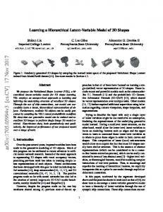
sjk = latent saliency to person j of item k, tjk = latent opinion of person j on item k, and djk = latent responsiveness propensity of person j for item k, meaning that person's interest in responding even if she does not have a strong opinion. Figure 1 about here
The observed response yjk is determined by the LCVs as illustrated in Figure 1, which describes the following process. Person j is confronted with item k. If the item is not salient (sjk < 0), then she gives an NA response to item k indicating that she considers the item irrelevant or lacks knowledge about the item. If the item is salient (sjk � 0), and if she feels strongly positive (tjk � CU ) or strongly negative (tjk � CL ), where CL and CU are cuto�s which are components of �2 , then she gives an ordinal response: a strong opinion will always be voiced. If the question is salient, and the opinion score is in the indi�erence zone (CL � tjk < CU ), she gives an ordinal opinion if she is responsive for that question (djk � 0), i.e. willing to express even a mild opinion, and gives an NA otherwise. Finally, if the person expresses an opinion, it is determined by the latent opinion variable tjk and a set of ordered cuto�s c (which are also components of �2 ) for the responses, 1 = c0
> < Prob(sjk < 0) + Prob(sjk � 0; crL � tjk � crU ; djk < 0) if r=NA Prob(sjk � 0; cr 1 � tjk � cr ) if r > rU or r < rL > > : Prob(sjk � 0; djk � 0; cr 1 � tjk � cr ) if rL � r � rU 8 > > �( �s(jk) ) + (1 �( �s(jk) ))� > > > > < (�(crU �t(jk) ) �(crL �t(jk) )) � �( �d(j)) if r=NA (1 �( �s(jk) )) � (�(cr �t(jk) ) �(cr 1 �t(jk) )) if r > rU or r < rL (2) > > > (1 �( �s(jk) )) � (�(cr �t(jk) ) �(cr 1 �t(jk) ))� > > > : (1 �( � )) if r � r � r : L
d(j)
U
2.2 Level II: distributions of person and item parameters, [�1
j
�2
].
The parameter vector �1 = (�; ; � ) contains random e�ects whose population (prior) distributions are governed by �2 :
�j � N (x0�(j) � ; ��2 )
(3)
k � N (x0 (k) ; � 2 )
(4)
�j � N (x0� (j) � ; ��2 )
(5)
where x�(j) , x (k) , x� (j) are vectors of covariates for person j or item k believed to be relevant to the corresponding e�ects. This induces a regression structure for the predictions. Note that the combination of (5) and the Level I model for �s(jk) allows saliency to depend on both person covariates and person�item interactions.
2.3 Hyperpriors for parameters, [�2 ] The parameter vector �2 = ( s ; d ; � ; ; � ; ��2 ; � 2 ; ��2 ; c) consists of all the general parameters that govern the Level I and II distributions. Hyperpriors for �2 were chosen to 8
contain little information for the respective parameters so that posterior distributions are determined primarily by the observed data, but enough to ensure proper posteriors. The prior distribution of the cuto�s c for ordinal opinions is uniform with order constraints, [cr jcr 1 ; cr+1 ] � Unif(cr 1 ; cr+1); r = 1; : : : ; R 1; r 6= r0
(6)
with c0 = 1, cr0 = 0 for some arbitrarily chosen r0 (for identi cation), and cR = 1. The saliency and responsiveness covariates' slopes are given (improper) uniform prior distributions; results with a proper prior for these parameters were indistinguishable. The remaining parameters are given proper priors with parameters selected (speci c to each application) so the priors are vague relative to the amount of information in the data. The regression coe�cients are given multivariate normal priors � � N (0; a� � I ),
� N (0; a � I ), and � � N (0; a� � I ), where a� , a and a are chosen a priori, and the identity matrices are of dimension corresponding to the coe�cient vectors. The priors for the variance components are inverse Chi-square, �� 2 � �2g� , � 2 � �2g , and �� 2 � �2g� . The speci c hyperparameter priors for our application are discussed in Section 3.3.
3 Analysis of the DuPont Corporation 1992 Engineering Polymers Division Customer Satisfaction Survey 3.1 Description of the survey The DuPont Corporation 1992 Engineering Polymers Division (EPD92) Customer Satisfaction Survey (CSS) was typical of the over 130 surveys conducted in a corporation-wide e�ort to obtain feedback from customers and prospective customers. The questionnaire was administered through the mail by a third party with DuPont identi ed as the sponsor of the 9
study. A strati ed sample of 120 current and prospective customers was selected, of whom
J = 102 persons responded for an overall response rate of 85%. These persons accounted for over 90% of DuPont sales for the Engineering Polymers business and 91 di�erent corporations. In our analysis, we treat all respondents as independent, ignoring the fact that a few corporations had multiple respondents. The questionnaire consisted of K = 20 items of the form: How satis ed are you with your supplier's performance for | on a 1 to 10 scale, where 1 is extremely dissatis ed and 10 is extremely satis ed. The 20 questions were grouped into six categories: (1) product quality
(questions 1-4), (2) technical support (questions 5-7), (3) marketing support (questions 8-9), (4) supply and delivery (questions 10-16), (5) innovation (questions 17-19), and (6) price (question 20). No NA category was o�ered, but NA was coded when a person did not respond to an item. This information comprises ordinal matrix Y. Person covariates included job type, DuPont share of customer's total engineering polymers purchases, type of product purchased, and type of business. The levels of the covariates are given in Table 1; Table 1 about here
\REF" denotes the reference category for the dummy variable coding. Two dummy variables were omitted for product type because the 21 NYLON customers correspond exactly with the 21 NOSHARE customers (NYLON was an area of future expansion for the Engineering Polymers division). We use the same person covariates in each part of the model(saliency, opinion, and responsiveness); this information de nes X� = X� = Xd . The item covariate matrix X was de ned so that fx (jk) : k = 1; : : : ; K g; K equally spaced values with mean 0 and standard deviation 1. This linear contrast indicates whether the mean item response varies inversely with the order of question administration (Green, 1984). 10
The saliency model covariate matrix Xs includes two predictors representing the relationship between job type and possession of the necessary knowledge to respond to certain items. We de ne x0s(jk) = (xs(jk)1 ; xs(jk)2 ) where xs(jk)1 = 1 if person j and item k are both
technically oriented and 0 otherwise, and xs(jk)2 is similarly de ned for sales orientation. Executive, marketing and purchasing job types were regarded as sales oriented, as were marketing support and supply/delivery question domains. Manufacturing and technical job types were regarded as technical, as were quality, technical support, and innovation question domains. With this speci cation, the coe�cients s of the saliency model measure the e�ect of domain expertise on saliency and thus on the prevalence of ordinal responses.
3.2 DuPont's Standard Analysis Before we provide the results of our model applied to the data, we present a subset of the \standard analyses" and inferences (as seen by the rst author) that was implemented by DuPont's Corporate Marketing and Business Research Division in 1992. The standard analysis provides both a benchmark in which to compare our model-based results (Section 3.3) as well as the primary motivating factor for this research; high cost for a simplistic analysis with poorly summarized results. For example, this study had a cost of roughly $30,000 and the \summary" output consisted of a 75 page book of cross-tabulated counts. A descriptive look at margin results for the EPD92 data (see Table 2)
Table 2 about here
indicates that most of the responses (79.0%) are either 8,9, or 10, which DuPont regards as \satis ed". A smaller proportion (12.6%) of the scores are from 4 to 7 (\somewhat satis ed") and 2.5% are less than 4 (\unsatis ed"). These de nitions led to choosing the indi�erence zone [crL ; crU ] as [4; 7] to conform to DuPont's somewhat satis ed group. The 11
corporate goal as of 1992 was 90% satis ed responses with no more than 5% unsatis ed; the Engineering Polymers division failed this standard. NA responses were 5.9% of all responses. Only 66 out of the 102 persons answered all 20 items. One respondent (case 96) answered only two out of 20 items, with a mean score of 3.5 (the lowest among all 102 respondents). Eleven out of the 102 respondents had mean rating less than 7. The innovation items (17-19) have the lowest mean responses among the questions, and the NA response rate is less than 15% for all items except question 14. Questions 9 and 20 had the lowest NA response rate of 1/102. The inferences and action plan DuPont derived from the margin results were that: (i) based on low means for items (17-19) DuPont was not perceived as an innovative company by these customers, (ii) the percentage of NA responses is low overall however does vary signi cantly by question, and (iii) there is a non-trivial proportion of unsatis ed customers speci cally customer 96. Further standard analyses which DuPont performed are cross-tabulated results such as those given in Table 1 columns (1)-(3). In columns (1) - (3) we present the average of the non-NA ratings, percentage of NA responses, and sample size for outcome matrix Y cut by each of the demographic categories. Columns (4) and (5), correspond to our model-based estimates described and used for comparison in Section 3.3. The inferences DuPont derived from these results are (iv) there is an extremely high non-response rate of 13.8% among NOSHARE (0% purchases from DuPont) customers, (v) HIGH share (70-99%) customers give higher mean ratings than MAJOR (100%) share customers while LOW (1-69%) share customers give lower ratings than NOSHARE customers, (vi) customers who buy DuPont RYNITE have extremely low mean ratings (7.61) and a corresponding low NA rate (1.7%) whereas DuPont HYTREL customers have a high mean rating (9.02) and low NA rate (1.0%), and (vii) respondents whose job type is TECHNICALLY oriented give lower mean ratings than other job types with a high NA rate of 9.5%. 12
Inference (iv) was expected by DuPont and suggests that saliency (as our model suggests) may play a signi cant role in determining NA status. DuPont managers attributed (v) to the fact that DuPont often takes MAJOR share customers for granted while really trying to placate HIGH share customers. Furthermore, LOW share customers have knowledge of DuPont, often negative, and would have the lowest opinion of the company as a whole. Inference (vi) lends credence to our indi�erence model, and in actuality it was DuPont managers description of this phenomenom that led to the development of the indi�erence zone formulation. Inference (vii) was attributed to the fact that technically oriented customers tend to be more critical when giving ratings and more honest about their lack of knowledge when it exists. Each of the inferences (i) - (vii) derived from the margin and cross-tabulated standard analysis will be re-considered using our model-based results presented next. A set of additional model-based results not obtained via DuPont's standard analysis will also be presented.
3.3 Bayesian analysis: speci cation and implementation The primary goal of our model-based analysis is to estimate the posterior distributions of model parameters and to summarize them by computing posterior point and interval estimates. These support inferences about person e�ects for saliency and opinion, item e�ects for opinion, covariate e�ects on saliency, opinion, and responsiveness, and the magnitudes of the variance components for the various populations of e�ects. Extensions include ranking of respondents or items, prediction, and grouping of respondents. We will compare our model-based inferences derived from estimates of the posterior distribution to DuPont's standard analysis. Samples from the posterior distributions [�1 jY] and [�2 jY] were obtained using the three versions of a Markov Chain Monte Carlo sampler, described in the Appendix. The reported results are based on combined analysis of draws from all of the samplers, after discarding 13
the initial part of each chain before it was estimated to have converged. Values of hyperprior parameters were chosen to be slightly informative to ensure proper posteriors. To identify the model we xed cuto� c7 a central data value. Initially, we xed cuto� c1 as in Albert and Chib (1993) however the sparse data in this range of the ordinal scale led to draws with high within series autocorrelation.
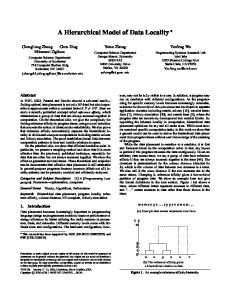
3.4 Bayesian analysis: inference A summary of results from the MCMC samplers are given in Table 1 columns (4)-(5), and Figure 2 panels (a) - (c). The model-based results reported in Table 1 are the posterior medians for the person opinion covariate slopes � and person saliency covariate slopes � . As they measure the e�ect of demographic pro le on opinion and saliency, we compare their estimated quantities to the sample based quantities of opinion and saliency (Y� and % NA) cut by demographic pro le (given in Table 1 (1) - (2)) derived in DuPont's standard analysis. Agreement of the standard analysis and our model-based estimates would be indicated by higher values of Y� associated with higher values of � and higher values of % NA responses associated with lower values of � . Figure 2(a) contains a plot of the ranks of the 102 person means Y�j� (where the mean is over the ordinal scores) against the ranks of the 102 posterior median person opinion e�ects �^j . The 45 degree line shown indicates equality of the ranks. Each point where the change in rank is greater than 5 is plotted with its case number so that it can be identi ed for further analysis. All other points are plotted with a \*". Agreement of the model-based ranks and standard analysis ranks would be indicated by the a tight scatter around the equality line with little change in orderings of the ranks. A plot of the 20 item means Y��k and posterior median item e�ects ^k is given in Figure 2(b). Each item is plotted with its item number. Figure 2(c) contains a plot of case index 1-102 versus the posterior probability of each case being in the bottom 10% in terms of overall rating. The solid horizontal line indicates a 50% probability. Each case with posterior probability 14
greater than 50% is plotted using its case number, all other cases are plotted with a \*". We next discuss how inferences derived from these model-based summaries con rm and/or refute the DuPont standard analysis inferences (i)-(vii) given above. Additional inferences from the MCMC sampler are also described.
Figure 2 about here
Posterior intervals for the k (item e�ects) are narrowest, followed by those for the �j (person opinion e�ects), and then the � 's (person saliency e�ects). This is sensible because there are 102 responses for each item but only 20 for each person; furthermore, saliency is observed only indirectly and is binary rather than ordinal. The posterior median item e�ects j for the innovation category (parameter indices 119-121) are lowest among the item e�ects, consistent with the low observed mean responses on these questions. We consider in Section 5 the implications of the low scores for this category. The \shrinkage" feature of the model is illustrated by comparison of respondents 96 and 53. The estimated opinion score e�ect �~96 for case 96, which had 18 NA responses and an observed mean of 3.5 (the lowest), was shrunk heavily towards its prior mean and now has only the eighth smallest median person opinion e�ect, �~96 = 1:844. Respondent 53, who gave 19 scores with mean 5.05 and only one NA, now has the lowest posterior median,
�~53 = 1:183, with a wide interval re ecting comparatively little information. Respondent 96 also has the lowest posterior median saliency parameter, �~96 = :092, and respondent 22 (with 0 NAs) has the greatest (but still nite) posterior median for saliency, �~22 = 5:213. Tables ?? and ?? show quantiles for the remaining (level 2) parameters; in the following discussion we give posterior probabilities of various events involving these parameters. This information can be interpreted to draw conclusions about general processes a�ecting the survey responses. 15
Tables ?? and ?? about here
The saliency covariate slopes are positive, Prob( s;1 > 0) = 0:970, Prob( s;2 > 0) = 0:992, meaning that persons nd questions more salient when the question asked is in an area of their expertise (or knowledge base). Furthermore, Prob( s;1 < s;2 ) = 0:925, showing that this e�ect is stronger for the technical area than for the sales area. This might occur because speci c technical knowledge is needed to answer technical questions whereas any person with general familiarity with a company might answer sales-related items. MAJOR share customers overall tend to nd questions more salient than other share groups, all of which nd questions more salient than the no-share group ( ~�;2 > ~�;4 ; ~�;3 > 0 with posterior probabilities around 0.7{0.9 for each parameter inequality). This is consistent with a positive relationship between saliency and length or size of business relationship. Noting that ~d;2 � ~d;3 0)=0.913, and Prob( d;4 > 0)>0.999), we further conclude that no-share persons (the baseline category) tend to be less likely than others to respond when indi�erent. By job type, Manufacturing persons tend to be the least likely to respond when indi�erent as shown by the medians ( ~d;10 = 2:560 < ~d;9 ; ~d;11; ~d;12 ) and posterior probabilities close to 1 for each comparison. The HIGH share customers tend to give the highest rating scores followed by MAJOR share, LOW share, and then NO share ( ~�;3 > ~�;2 > ~�;4 > 0, and posterior probabilities of 0.7{0.98 for the various comparisons). One possible explanation is that DuPont puts more e�ort into satisfying HIGH share customers than other groups as a whole. MAJOR customers have long standing relationships and may sometimes be taken for granted. LOW 16
share customers typically do not have the potential to generate greater sales and are given little e�ort. There is no evidence for a fatigue e�ect on the scores by item, since posterior interval for ~ ;1 is centered near 0 (Table ??) with Prob( ;1 > 0)=0.502.
4 Model sensitivity 4.1 Case in uence analysis In this section, we describe estimation of the in uence of each respondent observation yj ; j = 1; : : : ; 102 on the posterior means of model parameters by comparing the full-data posterior mean �� based on [�jY] (Section 3.3) to the case-deleted posterior mean �� j based on [�jY j ] where Y j is the response matrix Y excluding row j . Those cases for which there are large di�erences between components of �� and �� j are considered in uential. This analysis helps us to ag individual responses that may have an excessive e�ect on parameter estimates. Furthermore, tracing the e�ect of respondents with distinctive data patterns helps us to understand the workings of the complex model. It should be noted that this is one of at least three possible case in uence analyses. One alternative is to calculate the in uence of various items on parameter estimates. We did not pursue this because the items actually included in the survey were regarded as representative of the topics on which DuPont was interested in getting consumer feedback. Another possibility is to treat each individual response (one respondent and one time) as a case; we regarded this level of analysis as too detailed to be of practical interest. Since draws from [�jY] have already been obtained, we can generate estimates of the means for [�jY j ] by importance reweighting with weights [�jY j ] = [Y j j�][�] = [y j�] 1 : j [�jY] [Yj�][�] Computing weights for each draw requires no extra programming for this model because 17
[Yj j�] is simply the contribution to the likelihood from observation j . The details of case in uence analysis of the DuPont data under the model presented here, and a discussion of alternative choices of importance weights, is given in Bradlow and Zaslavsky (1997). Therefore we only brie y summarize the case in uence results. Five in uential cases were identi ed graphically. Several cases with unusually low or unusually high mean ordinal scores were in uential on the intercept in the model for opinion scores, �1 . Cases with an unusually high number of NAs were in uential on the saliency model intercept, � 1 . One case had many scores in the indi�erence zone and only one NA; deleting this case decreased the intercept for responsiveness d1, and paradoxically increased the saliency model intercept in order to keep the overall predicted number of NAs on target. In general, the e�ects of the in uential cases were consistent with our understanding of the workings of the model.
4.2 Sensitivity to opinion score model speci cation In this section we consider the sensitivity of parameter estimates to the normal distribution speci cation for the latent opinion scores tjk . The normal distribution was chosen initially for computational convenience because the DAGS relies on the conjugacy of the latent normal scores and the model parameters. The logistic (more commonly used in the Rasch model) and extreme value link functions are alternatives to the Gaussian link which also have natural interpretations, corresponding to proportional odds and proportional hazards models respectively (McCullagh 1980). We investigate the logistic link, rescaled by a factor
p
of 4= 2� to equate the slopes of the normal and logistic CDFs at zero. Equating the slopes yields parameter estimates for the �j and k that are on a comparable scales for either link when the linear predictor is also near zero. Parameter estimates using the logistic link can be obtained by importance weighting as
18
in the case in uence analysis (Section 4.1). The importance weights are proportional to [�jY]� = [Yj�]� [�jY] [Yj�] where [�jY]� and [Yj�]� are conditional densities based on the logistic link. The largest of the normalized weights was 0.0095, so we concluded that importance weighting yielded adequate estimates of the posterior mean under the logistic speci cation. Estimates of � and are not very sensitive to the choice of link function, nor are the corresponding variance components ��2 and � 2 . Estimates of � tend to be smaller under the logistic model for larger values of � , and the variance for saliency e�ects ��2 is smaller under the logistic speci cation. These discrepancies are not surprising because the linear predictor for the saliency model is typically far from the value (zero) where the links are matched. The ranks of person, item, and saliency e�ects do not change under the logistic model; the observed rank correlations are 0.986, 0.956, and 0.915 for �; ; and � respectively. This suggests that the the form of the link has little e�ect on the inferences of interest.
5 Posterior predictive model checks and model expansion Posterior predictive model checks (Rubin 1984) may be used to examine whether the hypothesized model adequately describes various aspects of the observed data. Let S (Y) denote any univariate statistic of interest. Posterior predictive model checks assess the t of the model by referring S (Y) to the distribution of S in replicate data sets Y� sampled from the posterior predictive distribution [Y� jY]. Model de ciencies are revealed when S (Y) is extreme with respect to the predictive distribution. The model can then be improved to address the de ciency.
R
The posterior predictive distribution for a parametric model is of the form [Y � j�p ][�p jY ]d�p , 19
where �p is the full parameter vector or a subset of it. To draw from the posterior predictive distribution, we must rst decide which parameters to include in �p , i.e. which parameters to draw conditional on the data Y and which to draw from their distributions conditional on other parameters but not conditional on the data. This ambiguity in the speci cation of [Y � jY ] permits us to consider alternative speci cations of the predictive distribution, which correspond to di�erent hypothetical replications of the data. For the DuPont survey, we could replicate, under the model, possible responses by the same people for the same items. To do this we de ne �p = (�1 ; �2 ) so [Y� jY]
/
Z
[Y� j�� ][�1� jY; �2� ][�2� jY] d�� :
(7)
and all parameters are conditioned on the data. Because this is the most conditional possible check distribution, it is likely to have the smallest variance and therefore is most powerful for nding de ciences in the response model. On the other hand, this check can easily miss de ciencies in the Level 1 and 2 models, because the parameters in these models are drawn conditional on the original data set. Another hypothetical replication corresponds to drawing both a new sample of subjects (with the same covariate values as the current sample) and a new set of items. For this, we de ne �p = �2 ; only the hyperparameters are conditioned on the data so we would expect increased variability in the replicates S (Y � ). This approach tests the adequacy of both the response model and the speci cation of the random respondent and item e�ects. A third alternative treats the items as xed but draws new values of the person parameters under the model, thereby checking the speci cation of the respondent e�ects (�; � ). For this check, �p = (�2 ; ). Similarly, we might treat people as xed but the items as random, letting �p = (�2 ; �; � ). We did not pursue these because we were interested in checking for patterns in either respondent or item e�ects that were not captured by the model. Finally, a prior predictive check (Box 1980) de nes �p as a null vector, replicating under the prior and ignoring all information in the data. The prior check is not useful here because our 20
hyperpriors are intended to be vague rather than to realistically describe the process that generates our data set. Results for the fully conditional check distribution were uninteresting, indicating that we could not nd any obvious de ciencies in the response model. We therefore focus on checks of the speci cations of person and item e�ects with �p = �2 , using 200 draws of �1 and Y. A more detailed presentation of the results is given in Bradlow (1994). Six posterior predictive check test statistics Si (Y) were chosen. The rst four of these are (S1 ) variance of row spreads, (S2 ) variance of column means, (S3 ) number of non-NA respondents, and (S4 ) the percent satisfaction index. We do not expect these statistics to contradict the model because the model is designed speci cally to describe these features of the data. Two further checks are (S5 ) an indi�erence zone check, and (S6 ) maximal inter-question correlation; for these the t of the model to the observed data is in question. The variance of row spreads describes the varying extent to which respondents spread their responses across the ordinal scale, S1 (Y) = varj (maxk (yjk (r)) mink (yjk (r))). We found that S1 (Y) = 5:53, the observed value, lies at the 26th percentile of its check distribution, indicating an adequate model t to this aspect of the data. The variance of column means, S2 (Y) = vark (�y�ik ), describes item-to-item variability. We found that the observed value S2 (Y) = 0:18 lies at the 30th percentile of the check distribution. The adequacy of t for check statistic 2 is expected due to the inclusion of item speci c parameters in the model. The number of non-NA respondents (those who give ordinal scores to all items), S3 (Y) =
P 1(P 1(y = NA) = 0), has been tracked historically at DuPont to measure the strength j k jk of the relationship between DuPont and its clients. The observed S3 (Y) = 66 lies at the 82nd percentile of the distribution, indicating that the model typically predicts fewer nonNA respondents than was observed, but this discrepancy could easily be due to chance. 21
DuPont measures business performance with the percent satisfaction index, S4 (Y) =
1P J j 1(�yj� � 8), the percentage of respondents whose mean response is at least 8.
The
observed value S4 (Y) = 0:705 lies at the 51st percentile, indicating a good model t.
Another check lets us test whether the the indi�erence zone model improves on the description of NA responses compared to what would be obtained with the saliency part of the model alone. The di�erence in NA proportions is S5 (Y) = p1 (Y) p2 (Y) where p1 (Y) is the proportion of NA responses from respondents with at least one score in the indi�erence zone, and p2 (Y) is the same proportion for other respondents. The observed S5 (Y) = 0:016 lies at the 53rd percentile of the reference distribution, so the model is consistent with this feature of the data. To test whether a simpler model with no indi�erence zone might t the data just as well, we re- t the model without the indi�erence zone. We found that the observed value lies at the 82nd percentile of the modi ed distribution distribution, suggesting that the indi�erence zone part of the model has some explanatory power for NA responses but the simpler model could not be conclusively rejected by this test. The maximal interquestion correlation, S6 (Y) = maxk6=k (cor(y�k ; y�k )), is the maxi0
0
mum inter-item correlation based on available (non-NA) cases for each pair of items and is designed to detect surprisingly strong relationships between items. The observed S6 (Y) = 0:862, representing the correlation between items 8 and 9, was extreme relative to the predictive check distribution (for which the maximum value over all 200 draws was 0.657), indicating a lack of model t. The next two observed correlations, 0.819 for items 12 and 13 and 0.762 for items 6 and 7, are also extreme relative to the check distribution for the largest correlation. This result was not entirely unexpected as the items were known to fall into categories representing domains of satisfaction, and each of these pairs falls within a single category. To model within-category correlation, the latent opinion score model for tjk was modi ed
22
to include an e�ect �j;Q(k) for person j on items contained in category Q(k),
tjk � N (�j + k + �j;Q(k) ; 1):
(8)
where Q(k) is de ned by
8 > 1 > > > > 2 > > > 4 > > > > 5 > > :6
if k = 1; 2; 3; 4
(Product Quality)
if k = 5; 6; 7
(Technical Support)
if k = 8; 9
(Marketing Support)
if k = 10; : : : ; 16 (Supply and Delivery) if k = 17; 18; 19 (Innovation) if k = 20
(Price)
The random-e�ects distribution is normal, �j;Q(k) � N (0; ��2 ), with ��2 � �g�2 , g� = 0:5, as with the other person parameters. The model modi ed as in (8) includes the 274 original parameters and 613 additional parameters (612 �jq and one variance component) and therefore took substantially longer to t. The posterior predictive check test statistics S1 {S5 t essentially as described for the previous model. The observed S6 (Y) = 0:862 lies at the 83rd percentile of the new test statistic distribution, from which the extreme draws were 0.673 and 0.957, a clear improvement in t over the previous model.
6 Algorithms for Bayesian inference 6.1 Overview Because of the complexity of our models, we conduct inference by drawing samples from the joint posterior distribution [� j Y], using Monte Carlo Markov Chain simulation methods (Besag, Green, Higdon, and Mengersen 1995, Gilks et al. 1995). Each of our methods 23
generates a sequence of draws f�(t) ; t = 0; 1; : : :g, where the sampling distribution of �(t+1) depends only on �(t) and the data and is devised so that the limiting distribution of the sequence is the desired posterior distribution. Within each step �(t) ! �(t+1) , there is a series of substeps in which each component or set of components of � is drawn in turn. Two of our samplers are Gibbs samplers (Gelfand and Smith 1990). These algorithms alternately draw from full conditional distributions [�A j � A ; Y] where (�A ; � A ) is a partition of �, which includes �1 ; �2 and possibly some additional parameters that facilitate construction of the sampler. Within each step, every component of � appears at one substep as part of
�A . A third version of the sampler applies a Metropolis-Hastings step for some components (Roberts and Smith 1993), which draws from an approximation to the conditional distribution and corrects for the discrepancy between the sampling and target distribution through a rejection step. We now describe conditional distributions for parameters which are drawn in the same way in all three samplers. Several components of �2 have the conditional likelihoods of the standard normal linear model, with conjugate priors (multivariate normal for the regression coe�cients and inverse chi-square for the residual variance). These are the coe�cient vectors
� ; ; � and the corresponding variance components ��2 ; � 2 ; ��2 . For example, the conditional distribution of coe�cients � is multivariate normal with a mean that is a precision weighted average of the regression estimator and the hyperprior mean, [ � j � � ] � N ((�� 2 X�0 X� + a� 1 I ) 1 X�0 �; (�� 2 X�0 X� + a� 1 I ) 1 ):
(9)
The variance components are drawn from their conditional inverse chi-squared distributions, whose shape parameter is the sum of the number of observations and the hyperprior degrees of freedom. For example, de ning the residual sum of squares SS� = (� X� � )0 (� X� � ), then ��2 � (SS� + 1)=(J + g� ) � �J +2 g� . The conditional distributions of the remaining parameters, �1 = (�; ; � ); s ; d, and c, involve the likelihood (2), because the parameters appear there directly or through the
24
de nitions of �d(j) ; �s(jk) , and �t(jk) . Hence there is no direct, closed-form sampling distribution for these parameters, although the conditional densities can be calculated, up to a normalizing constant. The next subsections describe three di�erent methods for sampling from these distributions.
6.2 Adaptive Griddy Sampler One approach to sampling from these distributions is to sample from a grid of equally spaced values over an appropriately selected range, as in the Griddy Gibbs approach of Ritter and Tanner (1992). We implemented an adaptive algorithm to ensure proper centering and scaling of the grid, which we call an Adaptive Griddy Sampler (AGS). To draw each univariate parameter component, we initially center the grid at that parameter's previous draw, which due to the Markov structure, is likely to be close to the center of the current conditional distribution. We choose a grid width that makes the probability mass contained within the range of the grid close to 1, initially using a multiple of the unconditional standard deviation of the parameter estimated from previous draws, which must be at least as great as the conditional standard deviation. The conditional density is calculated at each point on the grid. The grid is then diagnosed as to its centering and scaling by computing (a) the grid point 1 � N max � N with maximum probability density, and (b) the ratio of the maximum density to a-th largest density value. If N max > NU or N max < NL the grid is not centered; then a new grid is calculated which is recentered at the grid value with maximum density. If the grid is centered, but the scaling ratio of the maximum to the a-th largest density value is larger than M , the scale of the grid is too wide (taking in too many points with very small density). Then we rescale the grid, shrinking its width by a factor of f . In our example, we used N = 50 grid points, centering bounds (NL ; NU ) = (15; 35), scaling cuto� a = 4 and ratio M = e 8 (equivalent to 4 standard deviations based on 25
approximate normality). An average of 1.5 recenterings were required per draw before the series converged, and very few thereafter. A grid approximation is also used to sample cr , but is simpler because the conditional support of cr is bounded due to the order restrictions on c. The grid therefore is anchored by the bounds. (For c0 and cR , the end of the grid which is unbounded is determined adaptively as described above.)
6.3 The Metropolis-Hastings Algorithm Another approach to the intractable conditional distributions is to replace the draw from the conditional distribution with a Metropolis step; the overall procedure is then a MetropolisHastings (MH) algorithm (Hastings 1970) which also converges to the desired stationary distribution. In general (and suppressing for readability the dependence of all conditional densities on the other parameters), a Metropolis step for a parameter ! with conditional distribution f proceeds by drawing !� from an approximating distribution g and then letting
8 > < !� ( t +1) ! => : !(t)
with probability min(1; w(!� )=w(!(t) )) otherwise
where w(!) = fg((!!)) , the importance ratio. In our implementation, the parameters were partitioned into their univariate components because an adequate approximating distribution g is di�cult to de ne in the highdimensional space of the multivariate parameters. The code for the AGS was used to numerically estimate the normal sampling approximation g by estimating the density-weighted mean and variance over the grid. This approximation is more robust to non-normality in the tails than the normal approximation based on posterior information at the posterior mode (Tierney, Kass, and Kadane 1991).
26
6.4 The Data Augmented Gibbs Sampler Another Gibbs sampling approach, based on Data Augmentation (Tanner and Wong 1987), uses a set of conditional distributions which are all in closed form. This set of conditional distributions is obtained by augmenting the parameter vector with LCV matrices S; T; and D. The resulting number of parameters is much larger, but all distributions are in closed form. The conditional distribution of each LCV is a truncated or untruncated normal, while the conditional distributions of the remaining parameters follow from the regression speci cations of the LCV distributions. We discuss this approach in detail because it illustrates how the method of Albert and Chib (1993) can be extended to handle the complex latent tree structure of the indi�erence zone model or similar models involving a complex observation process, and also because the LCVs are themselves legitimate objects of inference. We rst give details of the LCV distributions. The conditional distribution of a latent saliency score sjk combines its normal prior distribution with a likelihood and has three cases (again suppressing the conditioning variables on the left hand side):
8 > + > < N (�s(jk) ; 1) sjk � > N (�s(jk) ; 1) > :
if yjk 6= NA
(case 1)
if yjk =NA, CL � tjk � CU ; djk < 0 (case 2)
N (�s(jk) ; 1) otherwise
(case 3)
where N + (N ) is the positive (negative) part of the normal distribution. In case 1, an ordinal score is observed so the question must have been salient (sjk � 0). In case 2, an NA is observed, but the latent score tjk is in the indi�erence zone and the person is not responsive (djk < 0), so we would observe an NA, regardless of the value of sjk < 0. In Case 3, we observed an NA and know that it did not appear due to indi�erence; hence the NA must have occurred because sjk < 0, i.e. the question was not salient. The conditional distribution of a latent opinion score tjk is determined by the normal
27
regression model and the cuto� function r(�):
8 > > < N (�t(jk) ; 1) restricted to (cr 1; cr ) tjk � > N (�t(jk) ; 1) restricted to (CL ; CU ) > : N (�t(jk) ; 1) untruncated
if yjk = r
(case 1)
if sjk > 0 and yjk =NA (case 2) otherwise
(case 3)
Case 1 applies if there is an ordinal response. For case 2, if the person gives an NA response when the question is salient (sjk > 0), then tjk must be in the indi�erence zone (CL ; CU ). If the question is not salient, the response does not depend on tjk so the conditional distribution is the same as the prior distribution. The conditional distribution for the latent responsiveness score djk also involves three cases:
8 > + > < N (�d(j) ; 1) djk � > N (�d(j) ; 1) > : N (�d(j) ; 1)
if CL � tjk � CU ; yjk = r
(case 1)
if sjk � 0; CL � tjk � CU ; yjk =NA (case 2) otherwise
(case 3)
In case 1, the score is in the indi�erence region but the person gives an ordinal response and hence must have been responsive. In case 2, the question is salient but the person gives an NA and hence must have been unresponsive. Otherwise, the data provide no information about the value of djk . Conditional on the augmented data including S; T; and D, the conditional distributions for the remaining components of � (other than c) are posterior distributions of coe�cients in linear regression models. The conditional distributions of d and s are similar to those in (9), where for s the response variable of the regression is the residual sjk �j . The additive speci cation of �t(jk) further simpli es the conditional distributions of �j , k and
�j . In particular, �j � N ((K + ��
2) 1
K X k=1
2 x0
!
(tjk k ) + �� �(j) � ; (K + �� 2 ) 1 ); 28
a normal distribution with mean equal to a weighted average of the residuals and the prior mean from the regression for �j . Similarly
k � N ((J + � 2 ) and
�j � N ((K + ��
2) 1
0J 1 X 1 @ (t jk �j ) + � 2 x0 (j ) A ; (J + � 2 ) 1 ); j =1
K X k=1
(sjk
!
x0s(jk) s ) + �� 2 x0� (j) � ; (K + �� 2 ) 1 ):
The conditional distribution of each cuto� cr is uniform on the interval from the highest
tjk that must be below the cuto� to the lowest tjk that must be above the cuto�, subject to the order constraints on cuto�s (which may be relevant if a particular ordinal response never appears in the data). For all cuto�s 0 < r < R other than the bounds of the indi�erence zone or the xed cr0 ,
�
�
cr � Unif max(cr 1 ; ymax tjk ); min(cr+1 ; yjkmin t ) ; =r+1 jk jk =r
(10)
as in Albert and Chib (1993). For the indi�erence zone bounds, the cuto�s must also be consistent with NA cases which are known to be due to indi�erence. Hence,
�
�
crL 1 � Unif max(crL 2 ; max t ); min(crL ; yjkmin t ) ; =r+1 jk J jk
(11)
where J = f(j; k) : yjk = rL 1 or (yjk = NA and sjk > 0)g, and the distribution of crU is modi ed similarly. (Due to a programming error, (10) was used in tting our models where (11) was called for, but we are con dent that this made little di�erence for this data set.)
6.5 Comparison of algorithms For each method, three parallel series were run in order to diagnose convergence of the sampler (Gelman and Rubin 1992). The starting values used were identical for each of the three methods. Overdispersed starting values e 2; e0 ; and e1 for hyperprior variances
��2 ; � 2 ; ��2 were selected based on marginal distributions in a trial run. The initial cuto�s 29
c were uniformly spaced on [ 2; 2]. Storage limitations allowed us to save only each 20th
draw from the DAGS sampler. We compare the three iterative simulation methods, as applied to the DuPont data, in terms of time per iteration, rst order autocorrelation, and number of iterations to convergence (Table 3). Each draw from DAGS represents 20 iterations, but a single DAGS iteration took only about 2.8 seconds, a consequence of the fact that all required distributions are in closed form. The autocorrelation for DAGS also is for 20-iteration draws (roughly comparable in computing time to one MH draw), and would be much higher for single iterations. This is expected because the DAGS formulation includes extra parameters that are integrated out in the other formulations of the model. Finally, the MetropolisHastings algorithm converged the fastest, in terms of number of draws and computation time. Table 3 about here
To compare the computational e�ciency of the algorithms we estimated the variance of posterior estimates obtained using the draws from each sampler in a xed time (21,600 seconds or 6 hours) after diagnosing convergence by the Gelman-Rubin method. This comparison is a�ected by both the time per draw and the autocorrelation of the draws. Variances (under the distribution of a Monte Carlo sequence) of the estimated posterior mean and quantiles (2.5%, median, and 97.5%) were estimated assuming that a stationary time-series process generates the Gibbs sampling draws of each scalar parameter �i . Details of the computational methods and results are in Bradlow (1994). For most estimands the AGS has lower estimated variance than MH, even though the MH approach converged the fastest (Table 3). The DAGS and AGS were more nearly comparable: DAGS appeared to have smaller variances for most expectations and DAGS for most quantiles.
30
7 Summary The initial Bayesian model described via latent responsiveness, saliency and opinion variables and a latent decision tree extends current methods of analysis to allow for ordinal and \No Answer" (NA) responses. A conditional independence probit model for the observed response matrix Y combined with non-conjugate normal priors, normal hyperpriors, and inverse-gamma hyperpriors (Section 2.2) yields a joint posterior distribution which can be sampled from directly using any of three Markov Chain Monte Carlo formulations (Section 6). These methods were applied to a survey data set collected as part of the DuPont Corporation 1992 Continuous Improvement Program (Section 3). Inferences based on posterior samples obtained under the model are described in detail in Section 3.3 and three iterative computational schemes (Adaptive Griddy Sampler, Metropolis-Hastings, and Data Augmentation) are compared. An analysis of the sensitivity of parameter estimates to individual cases and to distributional assumptions was carried out using importance re-weighting (Sections 4.1 and 4.2). Also, a series of posterior predictive model checks indicated that the initial model failed to address the nesting of questions within categories. An augmented model including an e�ect for each of the item categories appeared to t quite well.
Bibliography Agresti, A. (1977), Considerations in measuring partial association for ordinal categorical data, Journal of the American Statistical Association, Vol. 72, 37-45. Albert, J.H., and Chib, S. (1993), Bayesian analysis of binary and polychotomous response data, Journal of the American Statistical Association, Vol. 88, 669-679. 31
Andrich, D. (1978), A rating formulation for ordered response categories, Psychometrika, Vol. 43, 561-573. (1980), A model for contingency tables having an ordered response classi cation, Biometrics, Vol. 35, 403-415.
Bahadur, R.R. (1961), A representation of the joint distribution of responses to n dichotomous items, Studies in Item Analysis and Prediction, 158-168, Stanford Univ. Press. Besag, J., Green, P., Higdon, D., and Mengersen, K. (1995), Bayesian computation and stochastic systems, Statistical Science, Vol. 10, 3-41. Birnbaum, A. (1968), A chapter in Statistical Theories of Mental Test Scores, AddisonWesley (Reading) by Lord, F.M., and Novick, M. Box, G.E.P. (1980), Sampling and Bayes inference in scienti c modeling and robustness, Journal of the Royal Statistical Society - Series A, Vol. 143, 383-430.
Bradlow, E.T. (1994), Analysis of ordinal survey data with \No Answer" responses, Doctoral Dissertation, Harvard University. Bradlow, E. T. and Zaslavsky, A. M. (1997), Case in uence analysis in Bayesian inference, Journal of Computational and Graphical Statistics, to appear.
Gelfand, A.E., and Smith, A.F.M. (1990), Sampling-based approaches to calculating marginal densities, Journal of the American Statistical Association, Vol. 85, 398-409. Gelman, A., and Rubin, D.B. (1992), Inference from iterative simulation using multiple sequences, Statistical Science, Vol. 7, 457-511. Gilks, W.R., Richardson, S., and Spiegelhalter, D. (1995), Practical Markov Chain Monte Carlo, Chapman and Hall: New York.
Green, P.E. (1984), Hybrid models for conjoint analysis: An expository review, Journal of Marketing Research, Vol. 21, 155-169.
32
Hastings, W.K. (1970), Monte Carlo sampling methods using Markov chains and their applications, Biometrika, Vol. 57, 97-109. Holland, P.W. (1981), When are item response models consistent with observed data?, Psychometrika, Vol. 46, 79-92.
(1990), On the sampling theory foundations of item response theory models, Psychometrika, Vol. 55, 577-601.
Lord, F.M. (1980), Applications of Item Response Theory to Practical Testing Problems, LEA publishers: Hillsdale, NJ. Masters, G.N. (1982), A Rasch model for partial credit scoring., Psychometrika, Vol. 47, 149-174. McCullagh, P. (1980), Regression models for ordinal data,, Journal of the Royal Statistical Society - Series B, Vol. 42, 109-142.
Rasch, G. (1960), Probablistic models for some intelligence and attainment tests, Copenhagen: Nielson and Lydiche (for Danmarks Paedagogiske Institut). Ritter, C., and Tanner, M.A. (1992), Facilitating the Gibbs sampler: The Gibbs stopper and the Griddy-Gibbs sampler, Journal of the American Statistical Association, Vol. 87, 861-868. Roberts, G.O., and Smith, A.F.M. (1993), Bayesian computation via the Gibbs Sampler and related Markov Chain Monte Carlo methods, JRSS-B, Vol. 55, 3-23. Rubin, D.B. (1984), Bayesianly justi able and relevant frequency calculations for the applied statistician, Annals of Statistics, Vol. 12, 1151-1172. Statistical Sciences Inc. (1993), S-Plus Reference Manual (Seattle). Tanner, M.A., and Wong, W.H. (1987), The calculation of posterior distributions by data augmentation, Journal of the American Statistical Association, Vol. 82, 528-540. 33
Tierney, L., Kass, R.E., and Kadane, J.B. (1991), Laplace's method in Bayesian analysis, Statistical Multiple Integration, American Mathematical Society, 89-99.
34
Table 1: Distributions of EPD92 covariates, observed means (Y� ), NA response rate (% NA), number of cases (n), and model-based estimated posterior medians of the covariate slopes ( � and � ) for person opinion and saliency scores. REF denotes the reference category for the dummary variable coding. Y� % NA n � � MAJOR 8.40 0.020 41 0.431 0.881 SHARE HIGH 8.58 0.060 22 0.590 0.337 LOW 7.96 0.056 18 0.069 0.493 NOSHARE 8.15 0.138 21 REF REF c
DELRIN 8.22 0.023 13 -0.264 0.420 c PRODUCT HYTREL 9.02 0.010 5 0.489 1.333 c /ZYTEL c 8.30 0.071 78 REF REF NYLON c RYNITE 7.61 0.017 6 -0.630 0.502 EXECUTIVE 8.24 0.041 23 0.076 1.447 MANUFACTURING 8.34 0.010 10 0.169 2.083 JOB TYPE MARKETING 8.29 0.100 4 0.000 0.960 PURCHASING 8.54 0.058 44 0.404 1.261 TECHNICAL 7.91 0.095 21 REF REF BUSINESS AUTOMOTIVE 8.34 0.021 17 -0.215 0.244 ENGINEERING 8.31 0.067 85 REF REF Table 2: Frequency table for response matrix Y
y
1 2 3 4 5 6 7 8 9 10 NA Frequency 19 11 21 17 81 47 113 638 519 454 120
35
Table 3: Computation Time and Mean Autocorrelation for iterative simulation methods Draws Draws until Draws used Seconds per Mean Method per chain convergence in inference iteration autocorrelation AGS 600 350 250 275 0.323 MH 800 300 500 73 0.748 DAGS 1500 750 750 56 0.374
sjk sjk � 0
sjk < 0
tjk
yjk = NA
tjk � CU or tjk � CL
CL < tjk < CU
yjk = r
djk djk � 0
djk < 0
yjk = NA
yjk = r
Figure 1: Latent tree diagram for a single response. The observed data are yjk , and the latent continuous variables are tjk , djk , and sjk ; cuto�s c, CL , and CU are components of general parameter �2 .
36
0
20
40
60
posterior probability
0.75
10 5 19 18 17
7
4
16 15 11 10 2
3
10
15
20
ranks of column means ( )
56 71 43 53
12
96
24 4
6
5
ranks of row means ( )
1
15
20
80 100
14 1 20 8 12 13
9 5
ranks of estimated gamma
100 80 60 40 20 0
ranks of estimated alpha
••••• ••••• • 102 7• •• 95 •55 • 372 27 •••66 • • 79 7792 •• 76 • 91 •54 23 •50 63 39••• • • 35 •••• 100•••••• •••20 48••••• 64 65 • •• •• •9 ••••• • • 96•••••• ••
85
14
0.50 •
•
0.25
0
•
• • • • • •••••••• •••••••••••••••••••••••••••••••••••••••••••••••••••••••••••••••••••••••••••• 0
20
40
60
80 100
case number (c)
Figure 2: Panel (a) contains a plot of the ranks of the 102 person sample means Y�j� versus ranks of the posterior median person opinion e�ects �^j . The 45 degree line indicates equality. The corresponding plot for the 20 item means Y��k and posterior median item opinion e�ects
^k is in panel (b). A plot of the posterior probability of each case being in the bottom 10% in terms of overall rating is given in panel (c). The horizontal line indicates 50% posterior probability. Each point is plotted using its case(item) number. 37