variable models. Latent variable analysis is a family of data modelling approaches that fac- torizes high-dimensional observations with a reduced set of latent ...
Heterogenous Data Fusion via a Probabilistic Latent-Variable Model Kai Yu, Volker Tresp Information and Communications, Siemens Corporate Technology, Otto-Hahn-Ring, 6 81730 Munich, Germany
Abstract. In a pervasive computing environment, one is facing the problem of handling heterogeneous data from different sources, transmitted over heterogeneous channels and presented on heterogeneous user interfaces. This calls for adaptive data representations keeping as much relevant information as possible while keeping the representation as small as possible. Typically, the gathered data can be high-dimensional vectors with different types of attributes, e.g. continuous, binary and categorical data. In this paper we present - as a first step - a probabilistic latent-variable model, which is capable of fusing high-dimensional heterogenous data into a unified low-dimensional continuous space, and thus brings great benefits for multivariate data analysis, visualization and dimensionality reduction. We adopt a variational approximation to the likelihood of observed data and describe an EM algorithm to fit the model. The advantages of the proposed model are illustrated on toy data and used on real-world painting image data for both visualization and recommendation.
1
Introduction
Among others, pervasive computing will be characterized by the processing of heterogeneous and high-dimensional data. For example, results provided by Internet search engines may contain text, pictures, hyperlinks, categorial and binary data. The demand for clearly structured information presented to end users, but also the limitations of telecommunication networks as well as user interfaces calls for a lower-dimensional representation providing the most relevant information. Promising candidates for this task of dimensionality reduction are latent variable models. Latent variable analysis is a family of data modelling approaches that factorizes high-dimensional observations with a reduced set of latent variables. The latent variables offer explanations of the dependencies between observed variables. An example is the probabilistic variant of the widely used principal component analysis, PPCA, where observations are explained by a linear projection of a set of Gaussian hidden variables, plus additive observation noise [10]. Standard PCA is widely used for data reduction, pattern recognition and exploratory
data analysis. Recent studies on PCA reveals its connections to statistical factor analysis (FA) [7]. While existing PCA or FA approaches rely on continuous-valued observations, data analysis on mixed types of data (discrete and continous observations) is often desirable: – In solving typical data mining problems, one is always faced with mixed data. For example, a hospital patient’s record typically includes fields like age (discrete real-valued), gender (binary), various examination results (real-valued or categorical), binary indicator variables for the presence of symptoms or even textual descriptions. A unified means to explore the dependencies of these data are needed. – If applied to dimensionality reduction for pattern recognition, PCA is purely unsupervised. Thus, the resulting projection can be not indicative of the targeted pattern distribution. A generalized PCA which allows class membership as additional attributes (binary or categorical) may obviously provide a better solution. – For heterogeneous data, it is often difficult to derive a small set of common features describing the total data. For example, in a web-based image retrieval system, each image can be characterized by its visual features, accompanying words, categories, and user visit records. For these reasons, we will present a probabilistic latent variable model to fit observations with both continuous and binary attributes in this paper. Since categorical attributes can always be encoded by sets of binary attributes1 (e.g. 1of-c coding scheme), this model can be applied to a wide range of situations. We call this model generalized probabilistic PCA, GPPCA. In the next section we describe the latent variable model and derive an efficient variational expectation-maximization (EM) formalism to learn the model from data. In Sec. 3 we discuss properties of the model and connections to previous work. In Sec. 5 we present empirical results based on toy data and image data, with focus on both data visualization and information filtering.
2
A Generalized Probabilistic PCA Model
The goal of a latent variable model is to find a representation for the distribution p(t) of observed data in an M -dimensional space t = (t1 , . . . , tM ) in terms of a number of L latent variables x = (x1 , . . . , xL ). In our setting of interest, we consider a total of M continuous and binary attributes. We use m ∈ R to indicate that the variable tm is continuous-valued, and m ∈ B for binary variables (i.e. {0, 1
To be precise, an additional constraint is required here, which we drop for simplicity.
1}). The generative model is: x ∼ N (0, I) y|x = W T x + b tm |ym ∼ N (ym , σ 2 ) � tm |ym ∼ Be g(ym )
m∈R m∈B
(1) (2) (3) (4)
By Be(p) we denote a Bernoulli distribution with parameter p (the probability of giving a 1). W is an L × M matrix with column vectors (w1 , . . . , wM ), b an M -dimensional column vector, and g(a) the sigmoid function g(a) = 1/(1 + exp(−a)). We assume that observed vectors t are generated from a prior Gaussian distribution with zero mean2 unit covariance. Note that we assume a common noise variance σ 2 for all continuous variables. To match this assumption, we sometimes need to use scaling or whitening as a pre-processing step for the continuous data in our experiments. The likelihood3 of an observation vector t given the latent variables x and model parameters θ is p(t|x, θ) = p(tR |x, θ)p(tB |x, θ) n 1 (y − t )2 o Y Y � 1 m m √ = exp − g (2tm − 1)ym 2 2 2 σ 2πσ m∈R m∈B
(5)
where ym = wTm x + bm . The distribution in t-space, for a given value of θ is then obtained by integration over the latent variables x Z p(t|θ) = p(t|x, θ)p(x)dx (6) For a given set of N observation vectors, the log likelihood of data D is L(θ) = log p(D|θ) =
N X
log p(tn |θ)
(7)
n=1
We estimate the model parameters θ = {W , b, σ 2 } using a maximum likelihood approach, which can be achieved by the expectation-maximization (EM) algorithm. However, given parameters θ estimated from the previous M-step, the integral Eq. (6) in the E-step can not be solved analytically. We thus have to resort to an approximated solution. Previous work on mixed latent variable models has concentrated, for example, on approximating the (equivalent of the) integral Eq. (6) by Monte Carlo sampling [6] or by Gauss-Hermite numerical integration [8]. These approaches demonstrate good performance in many cases, but introduce a rather high computational cost. In the next section, we will present a variational approximation to solve this problem. 2
3
A non-zero mean and non-identity covariance matrix can be moved to parameters W and b without loss of generality. A full Bayesian treatment would require prior distributions for the parameters θ. We do not go for a full Bayesian solution here, thus implicitly assuming a non-informative prior.
2.1
A Variational EM Algorithm for Model Fitting
In order to select the parameters θ that maximize Eq. (7), we employ a variational EM algorithm. A variational EM algorithm constructs a lower bound (the variational approximation) for the likelihood of observations, Eq. (7), by first introducing additional variational parameters ψ. Then, it iteratively maximizes the lower bound with respective to the variational parameters (at the E-step) and the parameters θ of interest (at the M-step). This idea has been applied by Tipping [9] to a hidden-variable model for binary data only. A variational approximation for the likelihood contributions of binary variables, tm ∈ B in Eq. (4) is given by p(tm |x, θ) ≥ pe(tm |x, θ, ψm ) � 2 = g(ψm )exp (Am − ψm )/2 + λ(ψm )(A2m − ψm )
(8)
where Am = (2tm − 1)(wTm x + bm ) and λ(ψm ) = [0.5 − g(ψm )]/2ψm . For a fixed value of x, we get the perfect approximation where the lower bound is maximized to be p(tm |x, θ) by setting ψm = Am .4 The variational approximation for the log likelihood Eq. (7) of data D becomes L(θ) ≥ F(θ, Ψ ) = log
N Z Y
pe(tn |x, θ, ψ n )p(x)dx
(9)
n=1
where pe(tn |x, θ, ψ n ) =
Y m∈R
p(tmn |x, wm , σ)
Y
pe(tmn |x, wm , ψmn )
(10)
m∈B
We denote the total set of N × |B| variational parameters by Ψ . Since the variational approximation depends on x only quadratically in the exponent and the prior p(x) is Gaussian, the integrals to obtain the approximation F(θ, Ψ ) can be solved in closed form. The variational EM algorithm starts with an initial guess of θ and then iteratively maximizes F(θ, Ψ ) with respect to Ψ (E-step) and θ (M-step), respectively, holding the other fixed. Each iteration increases the lower bound, but will not necessary maximize the true log likelihood L(θ). However, since the E-step results a very close approximation of L(θ), we expect that, at M-step, the true log likelihood is increased. Details are given in the following: (i) E-step: Ψ k+1 ← arg maxΨ F(θk , Ψ ). The optimization can be achieved by a normal EM approach. Given ψ old updated from the previous step, the n algorithm iteratively estimates the sufficient statistics for the posterior approxi5 mation p˜(xn |tn , θk , ψ old n ) , which is again a Gaussian with covariance and mean 4
5
However, in the case of x distributed over a Gaussian prior N (0, I), maximization of the corresponding lower bound with respect to ψm is not straightforward. Based on Bayes’ rule, the posterior approximation is derived by normalizing pe(tn |xn , θk , ψ old n )p(xn ) and thus is a proper density, no longer a lower bound.
given by Cn =
X �1 X �−1 T old w w + I − 2 λ(ψmn )wm wTm m m σ2 m∈R
(11)
m∈B
n1 X o X � 2tmn − 1 � old (tmn − bm )wm + + 2bm λ(ψmn ) wm (12) 2 σ 2 m∈R m∈B � and then updates ψ n by maximizing En log pe(tn , xn |θk , ψ n ) where the expec� tation is with respect to p˜(xn |tn , θk , ψ old p(tn , xn |θk , ψ n ) n ). Taking the derivative of En loge with respect to ψ n and setting it to zero leads to the updates � 2 ψmn = En (wTm xn + bm )2 = wTm En (xn xTn )wm + 2bm wTm En (xn ) + b2m (13) µn = Cn
where En (xn xTn ) = C n + µn µTn and En (xn ) = µn . The two-stage optimization updates ψ and monotonously increases F(θk , Ψ ). The experiments showed that this procedure converges rapidly, most often in only two steps. (ii) M-step: θk+1 ← arg maxθ F(θ, Ψ k+1 ). Similar to the former E-step, this can also be achieved by iteratively first estimating the sufficient statistics of p˜(xn |tn , θold , ψ k+1 Eq. (11) and Eq. (12), and then maximizing n ) through � PN k+1 E loge p (t , x |θ, ψ ) with respect to θ, where En (·) denotes the exn n n n n=1 pectation over p˜(xn |tn , θold , ψ k+1 n ). For m ∈ R, we derive the following updates wTm =
N hX n=1
σ2 =
(tmn − bm )En (xn )T
N ih X
i−1 En (xn xTn )
(14)
n=1
N �o 1 Xn X � T wm En (xn xTn )wm +2(bm −tmn )wTm En (xn )+(bm −tmn )2 N |R| n=1 m∈R
(15) where bm , m ∈ R, is directly estimated by the mean of tmn . For m ∈ B, we have the following updates (wTm , bm )T
N N hX i−1 h X i T bn ) =− 2λ(ψmn )En (b xn x (tmn − 0.5)En (b xn ) n=1
(16)
n=1
b n = (xT , 1)T . where x 2.2
Inference
Finally, given the trained generative model, we can infer the a posteriori distribution of hidden variables for a complete observation vector t by using Bayes’ rule p(t|x, θ)p(x) p(x|t, θ) = R (17) p(t|x, θ)p(x)dx
However, since the integral is again infeasible, we need to derive a variational approximation by normalizing pe(t|x, θ, ψ)p(x), where ψ is obtained by maximizing the lower bound p˜(t|θ, ψ). For a vector ˆt of partial observations, we can still infer the posterior distribution in a similar way. If only continuous variables are observed, a normal posterior calculation can be employed, without the need for a variational approximation. This solution is the same as calculating the posterior based on the standard probabilistic PCA model [10].
3
Properties of Generalized Probabilistic PCA
The rows of the ML estimator W that relates latent to observed variables span the principal subspace of the data. The GPPCA model allows a unified probabilistic modelling of continuous, binary and categorical observations, which can bring great benefits in real-world data analysis. Also, it can serve as a visualization tool for high-dimensional mixed data in a two-dimensional latent variable space. Existing models currently only visualize either continuous [1] or binary data [9]. Also, like PPCA [10], GPPCA specifies a full generative model, it can also handle missing observations in a principled way. For pattern recognition tasks, GPPCA can provide a principled data transformation for general learning algorithms (which most often rely on continuous inputs) to handle data with mixed types of attributes. One such example, in the context of painting image recommender system incorporating visual features, artists, user ratings, will be shown in Sec. 5. Also, GPPCA can provide a principled approach to supervised dimensionality reduction, by allowing the target values as additional observation variables. GPPCA explores the dependence between inputs and targets via the hidden variables and maximizes the joint likelihood of both. It actually discovers a subspace of the joint space in which the projections of inputs have small projection loss and also have clear class distributions. A large number of methods have been developed to handle issue of supervised data reduction (see [4]), like partial least squares, discriminant analysis. However most of them, in general, can not handle missing data.
4
Relation to Previous Work
Jaakkola & Jordan [5] proposed a variational likelihood approximation for Bayesian logistic regression, and briefly pointed out that the same approximation can be applied to learn the “dual problem”, i.e. a hidden-variable model for binary observations. Tipping [9] derived the detailed variational EM formalism to learn the model and used it to visualize high-dimensional binary data. Collins et al. [3] generalized PCA to various loss functions from the exponential family, in which the case of Bernoulli variables is similar to Tipping’s model. Latent variable models for mixed observation variables were also studied by [6] and [8]. In contrast to our variational approach, [6] and [8] used numerical integration methods to handle the otherwise intractable integral in the EM algorithm. Latent variable
models for mixed data were already mentioned by Bishop [1] and Tipping [9], yet never explicitly implemented. Recently, Cohn [2] proposed informed projections, a version of supervised PCA, that minimizes both projection loss and inner-class dissimilarities. However, this requires tuning a parameter β to weight the two parts of the loss function,
5
Empirical Study
Fig. 1. A toy problem: PCA, GPPCA and GPPCA-W solutions
5.1
A Toy Problem
We first illustrate GPPCA on a simple problem, where 100 two-dimensional samples are generated from two Gaussian distributions with mean [−1, 1] and [1, −1] respectively and equal covariance matrices. A third binary variable was added that indicates which Gaussian the sample belongs to. We perform GPPCA, as described in Sec. 2, and standard PCA on the data to identify the principal subspace. The results are illustrated in Fig. 1. As expected, the PCA solution is along the direction of largest variance. The GPPCA solution, on the other hand, also takes the class labels into account, and finds a solution that conveys more information about the observations. In an additional experiment, we pre-process the continuous variables with whitening and then perform GPPCA. We will refer to this as GPPCA-W in the following. With GPPCA-W, the solution even more clearly indicates the class distribution. Clearly, a change of the subspace in W corresponding to the whitened continuous variables will no longer change the likelihood contribution. Thus, the GPPCA EM algorithm will focus on the likelihood of binary observations only and thus lead to a result with clear class distribution.
(a) PCA solution
(b) GPPCA solution
(c) GPPCA-W solution
Fig. 2. Visualization of painting images
5.2
Visualization of Painting Images
Next, we show an application of GPPCA to visualizing image data. We consider a data set of 642 painting images from 47 artists. An often encountered problem in the research on image retrieval is that low-level visual features (like color, texture, and edges) can hardly capture high-level information of images, like concept, style, etc. GPPCA allows to characterize images by more information than just those low-level features. In the experiment, we examine if it is possible to visualize different styles of painting images in a 2-dimensional space by incorporating the information about artists. As the continuous data describing the images, we extract 275 low-level features (correlagram, wavelet texture, and color moment) for each image. We encode the artists in 47 binary attributes via a 1-of-c scheme, and obtain a 322dimensional vector with mixed data for each image. The result of projecting this data to a 2-dimensional latent space is shown in Fig. 2, where we limit the shown data to the images of 3 particular artists. The solution given by normal PCA does not allow a clear separation of artists. In contrast, the GPPCA solution, in particular when performing an additional whitening pre-processing for the continuous features, shows a very clear separation of artists. Note furthermore, that the distinction between Van Gogh and Monet is a bit fuzzy here—these artists do indeed share similarities in their style, in particular brush stroke, which is reflected by texture features. 5.3
Recommendation of Painting Images
Due to the deficiency of low-level visual features, building recommender systems for painting image is a challenging task. Here we will demonstrate that GPPCA allows a principled way of deriving compact and highly informative features. Thus the accuracy of recommender systems based on the new image features can be significantly improved.
(a)
(b)
Fig. 3. Precision on painting image recommendation, based on different features
We use the same set of 642 painting images as in the previous section. 190 users’ ratings (like, dislike, or no rated) were collected through an online survey 6 . For each image, we combine visual features (275-dim.), artist (47-dim.), and a set of M advisory users’ ratings on it (M-dim.) to form an (322+M )-dimensional feature vector. This feature vector contains continuous, binary and missing data (because on average each user only rated 89 images). We apply GPPCA to map the features to a reduced 50-dimensional feature space. The rest of 190−M users are then treated as test users. For each test user, we hide some of his/her ratings and assume that only 5, 10, 20, or 50 ratings are observed. We skip one particular case if a user has not given that many ratings. Then we use the rated examples, in form of input (image features) – output(ratings) pairs, to train an RBF-SVM model to predict the user’s ratings on unseen images and make a ranking. The performance of recommendation is evaluated by the top-20 precision, which is the fraction of actually liked images among the top-20 recommendations. We equally divide the 190 users into 5 groups, pick one group as the group of test users and treat the other 152 users as advisory users. For each tested case, we randomize 10 times and calculate the mean and error bars. The results are shown in Fig. 3. Fig. 3(a) shows that GPPCA improves the precision in all the cases by effectively incorporating richer information. This is not surprising since the information about artists is a good indicator of painting styles. Advisory users’ opinions on a painting actually reflect some high-level properties of the painting from a different individual’s perspective. GPPCA here provides a princpled way to represent different information sources into a unified form of continuous data, and allows accurate recommendations based on the reduced data. Interestingly, as shown in Fig. 3(a), a recommender system working with direct combination of 6
http://honolulu.dbs.informatik.uni-muenchen.de:8080/paintings/index.jsp
the three aspects of information shows a much lower precision than the compact form of features. This indicates that GPPCA effectively detects the ‘signal subspace’ of high dimensional mixed data, while eliminating irrelevant information. Note that there are over 80 percent of missing data in the user ratings. GPPCA also provides an effective means to handle this problem. Fig. 3(b) shows that GPPCA incorporating visual features and artist information significantly outperforms a recommender sytem that only works on artist information. This indicates that GPPCA working on the pre-whitened continuous data does not remove the influence of visual features.
6
Conclusion
This paper describes generalized probabilistic PCA (GPPCA), a latent-variable model for mixed types of data, with continuous and binary observations. By adopting a variational approximation, an EM algorithm can be formulated that allows an efficient learning of the model parameters from data. The model generalizes probabilistic PCA and opens new perspectives for multivariate data analysis and machine learning tasks. We demonstrated the advantages of the proposed GPPCA model on toy data and data from painting images. GPPCA allows an effective visualization of data in two-dimensional hidden space that takes into account both information from low-level image features and artist information. Our experiments on an image retrieval task show that the model provides a principled solution to incorporating different information sources, thus significantly improving the achievable precision. Currently the described model reveals the linear principal subspace for mixed high dimensional data. It might be interesting to pursue non-linear hidden variable model to handle mixed types of data. This approach and its possibly extensions may provide the basis for - even adaptively - compactifying data representations in future pervasive computing environments thus increasing their performance and acceptance.
7
Acknowledgments
We would thank Dr. Rudolf Sollacher and Anton Schwaighofer for their very constructive comments to this work. References [1] Bishop, C. M., Svensen, M., and Williams, C. K. GTM: The generative topographic mapping. Neural Compuation, 10(1):215–234, 1998. [2] Cohn, D. Informed projections. In S. Becker, S. Thrun, and K. Obermayer, eds., Advances in Neural Information Processing Systems, 15. MIT Press, 2003. [3] Collins, M., Dasgupta, S., and Schapire, R. A generalization of principal component analysis to the exponential family. In T. K. Leen, T. G. Dietterich, and V. Tresp, eds., Advances in Neural Information Processing Systems, 13. MIT Press, 2001.
[4] Hastie, T., Tibshirani, R., and Friedman, J. The Elements of Satatistical Learning. Springer Verlag, 2001. [5] Jaakkola, T. and Jordan, M. Bayesian parameter estimation via variational methods. Statistics and Computing, pp. 25–37, 2000. [6] Moustaki, I. A latent trait and a latent class model for mixed observed variables. British Journal of Mathematical and Statistical Psychology, 49:313–334, 1996. [7] Roweis, S. and Ghahramani, Z. A unifying review of linear gaussian models. Neural Computaion, 11:305–345, 1999. [8] Sammel, M. D., Ryan, L. M., and Legler, J. M. Latent variable models for mixed discrete and continuous outcomes. Journal of the Royal Statistical Society, Series B 59:667–678, 1997. [9] Tipping, M. E. Probabilistic visualization of high-dimensional binary data. In M. S. Kearns, S. A. Solla, and D. A. Cohn, eds., Advances in Neural Information Processing Systems, 11, pp. 592–598. MIT Press, 1999. [10] Tipping, M. E. and Bishop, C. M. Probabilistic principal component analysis. Journal of the Royal Statisitical Scoiety, B(61):611–622, 1999.