In this paper, we present a novel histogram den- sity modeling approach that models the emotion distribution by a 2-D histogram over the quantized VA space ...
A HISTOGRAM DENSITY MODELING APPROACH TO MUSIC EMOTION RECOGNITION Ju-Chiang Wang1,2 , Hsin-Min Wang2 , and Gert Lanckriet1 1
Department of Electrical and Computer Engineering, UC San Diego 2 Institute of Information Science, Academia Sinica ABSTRACT
Music emotion recognition is concerned with developing predictive models that comprehend the affective content of musical signals. Recently, a growing number of attempts has been made to model the music emotion as a probability distribution in the valence-arousal (VA) space to better account for the subjectivity. In this paper, we present a novel histogram density modeling approach that models the emotion distribution by a 2-D histogram over the quantized VA space and learns a set of latent histograms to predict the emotion probability density of a song from audio. The proposed model is free from parametric distribution assumptions over the VA space, easy to implement, and extremely fast to train. We also extend our model to deal with the temporal dynamics of timevarying emotion labels. Comprehensive performance study on two larger-scale datasets demonstrates that our approach achieves comparable performance to the state-of-the-art ones, but with much better training and testing efficiency. Index Terms— Affective computing, music information retrieval, subjectivity, temporal dynamics, emotion tracking 1. INTRODUCTION Recent years have witnessed increasing research interests in automatic music emotion recognition (MER), which holds the promise of managing the ever increasing volume of digital music in a content-based way [1, 2]. In a usual setting, a MER model is trained by machine learning to capture the mapping between musical features and emotion, and then the performance can be measured by the deviation between the predicted and ground truth emotions of a song [3–7]. Despite that considerable research has been undertaken in the past few years, MER still remains challenging. This can be attributed to two fundamental issues in modeling the music emotion: First, the perceived emotion in music is by nature subjective – it is typically highly dependent on the listener and the situational context [8–10]. Therefore, a deterministic approach that associates music with a single label might not work well in practice [11]. Second, the affective content of music changes temporally as the music evolves [12–16]. For This work was supported by Academia Sinica–UCSD Postdoctoral Fellowship to Ju-Chiang Wang.
better performance, it is desirable to consider the dynamic relationships between music and emotion. To handle the subjectivity issue, a growing number of attempts has been made to model the music emotion as a parametric probability distribution in the valence-arousal (VA) space [12, 17–19]. The underlying approaches typically assume that the VA emotion annotations from different listeners can be modeled by a bi-variate Gaussian distribution. While this permits analytical tractability, there is lack of consensus in the literature on whether the VA space is indeed Euclidean,1 and the parameter estimation could be biased if the annotation samples of a song are insufficient. An intuitive solution is to quantize the VA space into a G × G grid and train a predictive model for each cell independently [19]. Such approach is usually referred to as heatmap [14]. To tackle the problem of modeling the temporal dynamics of musical emotion, on the other hand, several sophisticated approaches have been proposed, such as Kalman filtering [13], Conditional Random Fields (CRF) [14], Continuous Conditional Random Fields (CCRF) [15], and Continuous Conditional Neural Fields (CCNF) [16]. Although notable progress has been made, relatively little effort has focused on optimizing the training efficiency scalable to a larger dataset. Moreover, the concept of time-varying emotion tracking lends itself to applications such as visualizing emotion in sync with music playback [1, 21]. It is thus important for a method to predict the emotion on local music signals in real time. In this paper, we propose the histogram density mixture (HDM) model, a novel probabilistic model that is interpretable and theoretically sound. The HDM-based approach models the emotion distribution of a song using 2dimensional histogram density estimation over the G × Gquantized VA space (cf. Fig. 1) and learns a mixture of latent histograms, each of which is associated with an audio topic. It makes emotion prediction on unseen audio by linearly combining the learned latent histograms with the weights generated from different audio topics. Our proposed model is free from parametric distribution assumptions over the VA space, easy to implement with the EM algorithm [22], extend1 One obvious problem is that the VA space in a typical interface for user to make the valence and arousal ratings is bounded, e.g. the one in [20] is bounded by [-1,1]. This may result in density discontinuity when modeling the annotation density around the boundaries.
Fig. 1. The histogram density distributions of the emotion annotations of four 30-second music excerpts in the VA space:2 (a) Splish Splash by Bobby Darin, (b) Dick Johnson by Pussy Galore, (c) American Gothic by David Ackles, and (d) Pledging My Love by Johnny Ace.
features of the song. Note that each probability xnk in xn is generated based on a specific audio topic ak . We will detail this process later in Section 3. Then, our goal is to learn K number of latent histograms H = {Φk }K k=1 , such that each Φk ∈ RG×G is associated with an audio topic ak . Let hn (i, j) and φk (i, j) denote the (i, j)-th element of Hn and Φk , respectively. We fit the HDM model by maximizing the log-likelihood of H on L defined as follows: XX X log p(H | L) = hn (i, j) log xnk φk (i, j) . (1) n
able to handle the temporal dynamics of emotion annotations, and extremely fast to train, and predicts emotion efficiently. We conduct performance study on two emotion annotated datasets, AMG1608 and MTurk. AMG1608 [23] is a newly complied dataset containing the emotion labels of 1,608 30second music excerpts annotated by 665 listeners. While, MTurk [24] is a widely used dataset for testing the performance of moment-by-moment emotion tracking. Our empirical result demonstrates that the proposed HDM approach achieves comparable performance to the state-of-the-art ones, but with much better training and testing efficiency. For reproductivity, the Matlab codes for implementing and evaluating HDM have been made publicly available.3 One can easily train a HDM model on 3,600 training instances within 2 second using a laptop computer. 2. THE HDM MODEL 2.1. Histogram density estimation for music emotion To account for the subjectivity nature of emotion perception, each song is typically annotated by multiple subjects. Let Y = [y1 , . . . , yU ] denote the set of annotations of a song, where yu ∈ R2 is the individual annotation of the u-th listener, and U is the number of annotations available for the song. Our approach starts with partitioning each emotion dimension equally into G bins and obtain a G × G grid representation of the VA space. Let H ∈ RG×G denote the 2-D histogram density for the grid, where h(i, j) denotes the probability of the (i, j)-th cell of H. We count the number of annotations in Y falling in the (i, j)-th Pcell P as initial h(i, j), and then normalize H by U such that i j h(i, j) = 1. Fig. 1 shows four examples of H. 2.2. Learning the latent histograms of HDM Suppose we have a labeled dataset L = {(Hn , xn )}N n=1 , where Hn is the histogram density matrix summarizing the annotations of the n-th song, and xn = [xn1 , . . . , xnK ], P k xnk = 1, is a probability vector that captures the acoustic 2 The VA space is ranging in between [-1,1] and quantized with G = 7. Its horizontal and vertical axes correspond to valence and arousal, respectively. 3 https://github.com/asriverwang/HDM_codes
i,j
k
To maximize log p(H|L) with respect to H, we apply the EM algorithm [22]. In the E-step, we compute xnk φk (i, j) . γ(k, n, i, j) ← P l xnl φl (i, j) In the M-step, we update H by P γ(k, n, i, j)hn (i, j) φ0k (i, j) ← P P n P . n q r γ(k, n, q, r)hn (q, r)
(2)
(3)
2.3. Modeling the temporal dynamics of emotion In the case of modeling the time-varying music emotion, emotion labels are annotated on local music signals consecutively (T ) (T ) (1) (1) over time. Let [(Hn , xn ), . . . , (Hn n , xn n )] denote the sequence of data tuples for the n-th song, where Tn is the length of the song. Our goal is to jointly model the rela(t) tionship between xn and its locally windowed emotion his(t+τ ) (t) (t−τ ) ], and to learn 2τ +1 , . . . , Hn , . . . , Hn tograms [Hn (r) K +1 (r) models {H(r) }2τ , where H = {Φ r=1 k }k=1 . (r) (t) Let hn (i, j) and φk (i, j) denote the (i, j)-th element of (r) (t) Hn and Φk , respectively. We derive the log-likelihood by log p(H(1) , . . . , H(2τ +1) | L, W ) = Tn X τ XX n
t=1 v=−τ
w(v)
X
h(t+v) (i, j) log n
i,j
X
(t) (v+τ +1)
xnk φk
(i, j) ,
k
(4) where the weights W = [w(−τ ) , . . . , w(0) , . . . , w(τ ) ] are set to descend from its center according to the power law: w(0) =1, w(±1) =0.5, w(±2) =0.25, and so on. We refer to this modified model as HDM dynamic (HDMd). The optimization problem of Eq. 4 can be divided into 2τ +1 sub-problems, each is in turn solved by the EM algorithm (cf. Eqs. 2 and 3). 2.4. Emotion prediction To make prediction with HDM, we can estimate the emoˆ = tion histogram density based on the probability vector x [ˆ x1 , . . . , x ˆK ] computed from the acoustic features of an unseen song: X ˆ = H x ˆ k Φk . (5) k
ˆ to represent the We can further compute the centroid of H mean of the emotion prediction for simplicity: X ˆ j)¯ µ= h(i, y(i, j) , (6)
a per-second basis using a graphical interface. The VA rating scale is normalized to [–0.5, 0.5] for making meaningful comparison with the result reported in [14].
i,j
4.2. Acoustic features ¯ (i, j) is the VA coordinate values of the (i, j)-th cell’s where y center. For time-varying emotion prediction with HDMd, ˆ (t) we compute the corresponding 2τ +1 histograms, given a x (t) ˆ v }τ {H v=−τ . Then, we re-estimate the histogram density at t by the weighted combination of the results predicted on its adjacent music signals {ˆ x(t+v) }τv=−τ : τ X ˆ (t+v) . ˆ (t) = P 1 w(v) H H v (v) w v v=−τ
(7)
3. ACOUSTIC FEATURE REPRESENTATION Suppose that a song contains a sequence of acoustic feature vectors computed over windowed frames of its audio signal, we apply a K-component Gaussian mixture model (GMM) to encode the acoustic feature vectors of the song into a probability vector x. Specifically, a GMM is pre-trained using the EM algorithm in an unsupervised manner on a large collection of acoustic feature vectors without emotion annotations [18]. By assigning each component of the GMM as an audio topic ak , we can compute a K-dimensional posterior probability vector that represents how likely the acoustic features of a frame is characterized by each audio topic [22]. As a song comprises multiple frames, we average the frame-level posterior probability vectors over the whole song to obtain x. Note that one can easily extend the frame-level features to blocklevel ones to compute the posterior probability vectors [25], so that more local temporal characteristics can be captured. 4. EXPERIMENTS 4.1. Dataset We adopt the AMG1608 and MTurk datasets for evaluating song-level MER and second-by-second emotion tracking, respectively. AMG1608 contains 1608 30-second music excerpts annotated by 665 subjects, and each excerpt is annotated by 15–32 subjects. During the song selection stage, the mood category information from All Music Guide (AMG) and a tag2VA algorithm [26] are applied to ensure that the emotions of the selected excerpts are well-balanced in the four quadrants of the VA space. Then, Amazon Mechanical Turk (AMT), an online crowdsourcing engine, is exploited to collect the emotion annotations, following previous work [3,14]. More details can be found in [23]. MTurk [24] is composed of 240 pieces of 15-second music clips drawn from the uspop2002 database. Each clip is annotated by 7 to 23 subjects via AMT. Each subject is asked to rate the VA values of 11 randomly selected music clips on
For AMG1608, we employ MIRToolbox [27] and YAAFE [28] to extract the frame-based acoustic features with a frame size of 50ms and 50% overlap. These features include MFCC-related (static, delta, and delta-delta MFCCs), tonal, spectral, and temporal features, leading to a 72-dimensional vector for a frame [23]. Then, we use the block-level representation [25] that consists of 16 consecutive frames, and each block overlaps with its previous one by 12 frames. A block-level feature vector is generated by concatenating the mean and standard deviation of the frame-based feature vectors. The block-level feature vectors are used to train the GMM and to compute the posterior probability vector x. For MTurk, we adopt the frame-based MFCCs (20-D) and spectral contrast (14-D) features provided by the authors of [24]. As the provided audio feature vectors contain only static features, we compute the delta- and delta-delta- features over the sequence of the static ones [29]. These dynamic features are concatenated to the static ones to add the information of the temporal dynamics of the audio signals. Since each emotion histogram is aligned with a specific one-second clip of a song, we extract the feature vectors from each onesecond clip. We use the frame-level (instead of block-level) feature vectors to train the GMM and to compute x(t) , as the audio signal for a x(t) is short (i.e., 1 sec). 4.3. Qualitative analysis of the learned models We depict the learned latent histograms on the entire AMG1608 with K=32 in Fig. 2, from which two observations are made. First, each latent histogram explains the semantic meaning of the corresponding audio topic. For example, T15, T16, and T26 are highly associated with the first quadrant of the VA space (e.g., happy, delighted topics), whereas T6, T19, and T32 are strongly correlated to the second (e.g., angry), third (e.g., sad), and fourth (e.g., calm) quadrants of the VA space, respectively. Second, one can qualitatively assess the quality of a latent topic. Some topics might be too vague to be useful for robust emotion modeling, such as T20 and T30. For better performance, some future study can be done to downweight or remove such latent topics accordingly. 4.4. Experimental result and discussion We stop the EM learning when the increase ratio of loglikelihood (cf. Eqs. 1 and 4) is smaller than 0.0001. We run our experiments on twelve cores of a server with a 2.66 GHz XEON X5650 CPU running Matlab R2011b on a 64-bit operating system. The average computing time on each train-test process is reported.
T1
T2
T3
T4
T5
T6
T7
T8
T9
T10
T11
T12
T13
T14
T15
T16
T17
T18
T19
T20
T21
T22
T23
T24
T25
T26
T27
T28
T29
T30
T31
T32
Fig. 2. The latent histogram topics (K=32) on AMG1608. Table 1. Performance comparison on AMG1608. Approach SVR-RBF [19] AEG [18] HDM (G=5) HDM (G=7) HDM (G=10)
ED 0.2895 0.2869 0.2887 0.2879 0.2899
R2 Val. 0.1409 0.1579 0.1419 0.1513 0.1490
R2 Aro. 0.6613 0.6686 0.6624 0.6652 0.6589
Time 20 min 15 min 0.3 sec 0.3 sec 0.4 sec
We perform 3-fold cross-validation on AMG1608 and use two metrics to measure the performance: the Euclidean distance (ED) and R2 (the coefficient of determination) [1] between the predicted VA values (i.e., µ) and the ground truth ones (the average VA ratings across the listeners of a song). ED is the smaller the better, while the opposite holds for R2 . We compare HDM with support vector regression (SVR) [30] and acoustic emotion Gaussians (AEG) [18]. The former, which stands for the baseline, is implemented by LIBSVM [31] along with RBF kernel and a grid parameter search to optimize its performance. The latter, which represents the state-of-the-art approach on AMG1608, uses the same setting as that of HDM to compute the acoustic feature representation of x.4 According to the cross-validation on the training set, we determine K=256 for both HDM and AEG. Table 1 presents the result for AMG1608. We also show the performance of HDM with different G values. From the result, HDM (G=7) significantly outperforms (p-value11 hr – >2 hr 35 min 1.4 sec
Table 2 shows the performance comparison of HDMd and HDM with different settings on MTurk, where “Contr.” stands for the spectral contrast feature, “dyn-” means using the concatenation of static, delta, and delta-delta features, and “stat-” uses only the static features. Three observations can be made. First, HDMd consistently outperforms HDM ˆ (t) ), sug(which makes independent prediction on each x gesting that our proposed method for modeling the temporal dynamics of emotion is effective. Second, “dyn-” consistently outperforms “stat-” regardless of any settings. This demonstrates the importance of using dynamic acoustic features in a codebook-like approach [32] (in our case, GMM). Third, MFCC features perform better in predicting the valence. In Table 3, we compare HDMd with other emotion tracking approaches on MTurk. For SVR, we follow the same setting in the AMG1608 case. AEG is trained with K=128 and ˆ (t) independently. We report the perforpredicts on each x mance of CRF in [14], and that of CCRF and CCNF in [16]. Note that the experimental settings for CCRF and CCNF [16] may be slightly different from ours. In general, the performance of HDMd is comparable to its competitors, but HDMd spends much lower computing time on training and testing. In particular, the superior performance of HDMd in RMS valence is remarkable. Such observation suggests HDMd a promising approach, as it is typically more difficult to model the valence perception from audio signals [1]. 5. CONCLUSION We have presented a novel probabilistic approach, coined as the histogram density mixture model, to model the relationship between emotion and music. We have also extended the model to handle the temporal dynamics of music emotion. Our experimental result has demonstrated its effectiveness and outstanding efficiency in training and prediction.
6. REFERENCES [1] Y.-H. Yang and H. H. Chen, Music Emotion Recognition, CRC Press, 2011. [2] Y. E. Kim, E. M. Schmidt, R. Migneco, B. G. Morton, P. Richardson, J. J. Scott, J. A. Speck, and D. Turnbull, “Music emotion recognition: A state of the art review,” in Proc. Int. Soc. Music Information Retrieval Conf., 2010, pp. 255–266. [3] T. Eerola, O. Lartillot, and P. Toiviainen, “Prediction of multidimensional emotional ratings in music from audio using multivariate regression models,” in Proc. Int. Soc. Music Information Retrieval Conf., 2009, pp. 621–626. [4] A. Huq, J. P. Bello, and R. Rowe, “Automated music emotion recognition: A systematic evaluation,” J. New Music Res., vol. 39, no. 3, pp. 227–244, 2010. [5] E. Schubert, “Modeling perceived emotion with continuous musical features,” Music Perception, vol. 21, no. 4, pp. 561– 585, 2004. [6] L. Lu, D. Liu, and H. Zhang, “Automatic mood detection and tracking of music audio signals,” IEEE Trans. Audio, Speech & Lang. Proc., vol. 14, no. 1, pp. 5–18, 2006. [7] M. Soleymani, M. N. Caro, E. Schmidt, C.-Y. Sha, and Y.-H. Yang, “1000 songs for emotional analysis of music,” in Proc. Int. Workshop on Crowdsourcing for Multimedia, 2013, pp. 1– 6. [8] M. Zentner and K. R. Scherer, “Emotional effects of music: production rules,” in Music and Emotion: Theory and Research, P. N. Juslin and J. A. Sloboda, Eds. Oxford University Press, New York, 2001. [9] K. R. Scherer, “Which emotions can be induced by music? what are the underlying mechanisms? and how can we measure them,” J. New Music Res., vol. 33, no. 5, pp. 239–251, 2004. [10] J. Hanratty, Individual and situational differences in emotional expression, Ph.D. thesis, School of Psychology, Queen’s University Belfast,, 2010. [11] Y.-H. Yang, C. C. Liu, and H. H. Chen, “Music emotion classification: A fuzzy approach,” in Proc. ACM Multimedia, 2006, pp. 81–84. [12] E. M. Schmidt and Y. E. Kim, “Prediction of time-varying musical mood distributions from audio,” in Proc. Int. Soc. Music Information Retrieval Conf., 2010, pp. 465–470. [13] E. M. Schmidt and Y. E. Kim, “Prediction of time-varying musical mood distributions using Kalman filtering,” in Proc. Int. Conf. Machine Learning and Applications, 2010, pp. 655– 660. [14] E. M. Schmidt and Y. E. Kim, “Modeling musical emotion dynamics with conditional random fields,” in Proc. Int. Soc. Music Information Retrieval Conf., 2011, pp. 777–782. [15] V. Imbrasait˙e, T. Baltruˇsaitis, and P. Robinson, “Emotion tracking in music using continuous conditional random fields and baseline feature representation,” in Proc. Int. Workshop on Affective Analysis in Multimeda, 2013. [16] V. Imbrasait˙e, T. Baltruˇsaitis, and P. Robinson, “CCNF for continuous emotion tracking in music: Comparison with CCRF and relative feature representation,” in Proc. IEEE Int. Conf. Multimedia and Expo Workshops, 2014.
[17] J. A. Russell, “A circumplex model of affect,” J. Personality and Social Science, vol. 39, no. 6, pp. 1161–1178, 1980. [18] J.-C. Wang, Y.-H. Yang, H.-M. Wang, and S.-K. Jeng, “The acoustic emotion Gaussians model for emotion-based music annotation and retrieval,” in Proc. ACM Multimedia, 2012, pp. 89–98. [19] Y.-H. Yang and H. H. Chen, “Prediction of the distribution of perceived music emotions using discrete samples,” IEEE Trans. Audio, Speech and Lang. Proc., vol. 19, no. 7, pp. 2184– 2196, 2011. [20] Y.-H. Yang, Y.-F. Su, Y.-C. Lin, and H. H. Chen, “Music emotion recognition: The role of individuality,” in Proc. ACM Int. Workshop on Human-Centered Multimedia, 2007, pp. 13–21. [21] J.-C. Wang, H.-M. Wang, and S.-K. Jeng, “Playing with tagging: A real-time tagging music player,” in Proc. IEEE Int. Conf. Acoustics, Speech & Signal Processing, 2012, pp. 77– 80. [22] C. M. Bishop, Pattern Recognition and Machine Learning, Springer-Verlag New York, Inc., 2006. [23] Yu-An Chen, Y.-H. Yang, J.-C. Wang, and H. H. Chen, “The AMG1608 dataset for music emotion recognition,” in Proc. IEEE Int. Conf. Acoustics, Speech & Signal Processing, 2015, [Online] http://amg1608.blogspot.tw/. [24] J. A. Speck, E. M. Schmidt, B. G. Morton, and Y. E. Kim, “A comparative study of collaborative vs. traditional musical mood annotation,” in Proc. Int. Soc. Music Information Retrieval Conf., 2011, pp. 549–554. [25] K. Seyerlehner, Content-Based Music Recommender Systems: Beyond simple Frame-Level Audio Similarity, Ph.D. thesis, Johannes Kepler University Linz, 2010. [26] J.-C. Wang, Y.-H. Yang, K. Chang, H.-M. Wang, and S.-K. Jeng, “Exploring the relationship between categorical and dimensional emotion semantics of music,” in Proc. Int. ACM workshop on Music Information Retrieval with User-centered and Multimodal Strategies, 2012, pp. 63–68. [27] O. Lartillot and P. Toiviainen, “A Matlab toolbox for musical feature extraction from audio,” in Proc. Int. Conf. Digital Audio Effects, 2007, pp. 237–244. [28] B. Mathieu, S. Essid, T. Fillon, J. Prado, and G. Richard, “YAAFE, an easy to use and efficient audio feature extraction software.,” in Proc. Int. Soc. Music Information Retrieval Conf., 2010, pp. 441–446. [29] S. Furui, “Speaker-independent isolated word recognition based on emphasized spectral dynamics,” in Proc. IEEE Int. Conf. Acoustics, Speech & Signal Processing, 1986, vol. 11, pp. 1991–1994. [30] Y.-H. Yang, Y.-C. Lin, Y.-F. Su, and H. H. Chen, “A regression approach to music emotion recognition,” IEEE Trans. Audio, Speech & Lang. Proc., vol. 16, no. 2, pp. 448–457, 2008. [31] C.-C. Chang and C.-J. Lin, “LIBSVM: A library for support vector machines,” ACM Trans. Intelligent Systems and Technology, vol. 2, pp. 27:1–27:27, 2011. [32] Y. Vaizman, B. McFee, and G. Lanckriet, “Codebook-based audio feature representation for music information retrieval,” IEEE/ACM Trans. Audio, Speech, & Language Processing, vol. 22, no. 10, pp. 1483–1493, 2014.