William T. Joines. John A. ..... 4.5 Snapshots of Ey on the plane y = 0 at t = 0.5 ns (left) by SEM with different .... Anita T. Layton for being my committee member and ...... [84] C. A. Kennedy, M. H. Carpenter, âAdditive Runge-Kutta schemes for.
A Hybrid Spectral-Element / Finite-Element Time-Domain Method for Multiscale Electromagnetic Simulations by
Jiefu Chen Department of Electrical and Computer Engineering Duke University Date: Approved:
Qing H. Liu, Supervisor
William T. Joines
John A. Trangenstein
Tomoyuki Yoshie
Anita T. Layton Dissertation submitted in partial fulfillment of the requirements for the degree of Doctor of Philosophy in the Department of Electrical and Computer Engineering in the Graduate School of Duke University 2010
Abstract (Electrical and Computer Engineering)
A Hybrid Spectral-Element / Finite-Element Time-Domain Method for Multiscale Electromagnetic Simulations by
Jiefu Chen Department of Electrical and Computer Engineering Duke University Date: Approved:
Qing H. Liu, Supervisor
William T. Joines
John A. Trangenstein
Tomoyuki Yoshie
Anita T. Layton An abstract of a dissertation submitted in partial fulfillment of the requirements for the degree of Doctor of Philosophy in the Department of Electrical and Computer Engineering in the Graduate School of Duke University 2010
c 2010 by Jiefu Chen Copyright All rights reserved except the rights granted by the Creative Commons Attribution-Noncommercial Licence
Abstract In this study we propose a fast hybrid spectral-element time-domain (SETD) / finiteelement time-domain (FETD) method for transient analysis of multiscale electromagnetic problems, where electrically fine structures with details much smaller than a typical wavelength and electrically coarse structures comparable to or larger than a typical wavelength coexist. Simulations of multiscale electromagnetic problems, such as electromagnetic interference (EMI), electromagnetic compatibility (EMC), and electronic packaging, can be very challenging for conventional numerical methods. In terms of spatial discretization, conventional methods use a single mesh for the whole structure, thus a high discretization density required to capture the geometric characteristics of electrically fine structures will inevitably lead to a large number of wasted unknowns in the electrically coarse parts. This issue will become especially severe for orthogonal grids used by the popular finite-difference time-domain (FDTD) method. In terms of temporal integration, dense meshes in electrically fine domains will make the time step size extremely small for numerical methods with explicit time-stepping schemes. Implicit schemes can surpass stability criterion limited by the CourantFriedrichs-Levy (CFL) condition. However, due to the large system matrices generated by conventional methods, it is almost impossible to employ implicit schemes to the whole structure for time-stepping. To address these challenges, we propose an efficient hybrid SETD/FETD method
iv
for transient electromagnetic simulations by taking advantages of the strengths of these two methods while avoiding their weaknesses in multiscale problems. More specifically, a multiscale structure is divided into several subdomains based on the electrical size of each part, and a hybrid spectral-element / finite-element scheme is proposed for spatial discretization. The hexahedron-based spectral elements with higher interpolation degrees are efficient in modeling electrically coarse structures, and the tetrahedron-based finite elements with lower interpolation degrees are flexible in discretizing electrically fine structures with complex shapes. A non-spurious finite element method (FEM) as well as a non-spurious spectral element method (SEM) is proposed to make the hybrid SEM/FEM discretization work. For time integration we employ hybrid implicit / explicit (IMEX) time-stepping schemes, where explicit schemes are used for electrically coarse subdomains discretized by coarse spectral element meshes, and implicit schemes are used to overcome the CFL limit for electrically fine subdomains discretized by dense finite element meshes. Numerical examples show that the proposed hybrid SETD/FETD method is free of spurious modes, is flexible in discretizing sophisticated structure, and is more efficient than conventional methods for multiscale electromagnetic simulations.
v
Contents Abstract
iv
List of Tables
vii
List of Figures
viii
List of Abbreviations and Symbols
ix
Acknowledgements
xi
1 Introduction
1
1.1
Problem Statement and Challenges . . . . . . . . . . . . . . . . . . .
1
1.2
Previous Methods for Time Domain Electromagnetic Simulations . .
3
1.2.1
The FDTD Method . . . . . . . . . . . . . . . . . . . . . . . .
3
1.2.2
The FETD Method . . . . . . . . . . . . . . . . . . . . . . . .
7
1.2.3
The DG-FETD and DG-SETD Methods . . . . . . . . . . . .
9
1.2.4
The Hybrid FDTD/FETD Method . . . . . . . . . . . . . . .
10
Dissertation Overview . . . . . . . . . . . . . . . . . . . . . . . . . .
11
1.3
2 Governing Equations and Finite Element Discretization Schemes
13
2.1
EBHD Scheme Based on Maxwell’s Equations . . . . . . . . . . . . .
13
2.2
EB Scheme Based on Maxwell’s Equations . . . . . . . . . . . . . . .
14
2.3
Vector Wave Equation Scheme . . . . . . . . . . . . . . . . . . . . . .
15
2.4
EH Scheme Based on Maxwell’s Equations . . . . . . . . . . . . . . .
16
vi
3 Non-Spurious Mixed Finite Element for Maxwell’s Equations 3.1
17
Mixed-Order Curl-Conforming Vector Basis Functions . . . . . . . . .
17
3.1.1
The Tetrahedral CT/LN Vector Element . . . . . . . . . . . .
18
3.1.2
The Tetrahedral LT/QN Vector Element . . . . . . . . . . . .
19
3.2
Non-Spurious Mixed Finite Element . . . . . . . . . . . . . . . . . . .
20
3.3
Galerkin’s Weak Form and Discretized System . . . . . . . . . . . . .
21
3.4
Numerical Results . . . . . . . . . . . . . . . . . . . . . . . . . . . . .
23
4 Non-Spurious Mixed Spectral Element for Maxwell’s Equations
25
4.1
Non-spurious Mixed Spectral Element . . . . . . . . . . . . . . . . . .
26
4.2
Galerkin’s Weak Form and Discretized System . . . . . . . . . . . . .
28
4.3
Numerical Results . . . . . . . . . . . . . . . . . . . . . . . . . . . . .
29
5 Dispersion Analysis for Mixed Finite Element Method
36
5.1
Mixed FEM System with Common Interpolation . . . . . . . . . . . .
36
5.2
Mixed FEM System with Mixed Interpolation . . . . . . . . . . . . .
40
5.3
Numerical Dispersion Analysis based on Rayleigh Quotient . . . . . .
41
6 Domain Decomposition Based on Discontinuous Galerkin Method 45 6.1
Galerkin’s Weak Form and Numerical Flux . . . . . . . . . . . . . . .
46
6.2
Treatment of Non-Conforming Meshes . . . . . . . . . . . . . . . . .
47
6.3
Multiple-Domain Discretized System . . . . . . . . . . . . . . . . . .
48
6.4
Well-Posed Perfectly Matched Layer . . . . . . . . . . . . . . . . . . .
51
7 Time Stepping Schemes for Multiple-Domain Discretized Systems 55 7.1
ERK for All Explicit Subdomains . . . . . . . . . . . . . . . . . . . .
56
7.2
IMEX-RK for Combination of Explicit and Implicit Subdomains . . .
58
7.2.1
Isolated Implicit Subdomains in IMEX-RK . . . . . . . . . . .
60
7.2.2
Coupled Implicit Subdomains in IMEX-RK . . . . . . . . . .
61
vii
7.2.3
Explicit Subdomains in IMEX-RK . . . . . . . . . . . . . . .
62
7.3
CN with block GS for All Implicit Subdomains . . . . . . . . . . . . .
62
7.4
Block Thomas Algorithm for Implicit Subdomains in 1D Array . . . .
63
8 Applications and Results
66
8.1
A Cavity Resonator Loaded with A Dielectric Ring . . . . . . . . . .
66
8.2
Measurement in A Reverberation Chamber . . . . . . . . . . . . . . .
68
8.3
Interconnect Package . . . . . . . . . . . . . . . . . . . . . . . . . . .
71
8.4
Antenna Array . . . . . . . . . . . . . . . . . . . . . . . . . . . . . .
74
9 Conclusion and Future Work
79
9.1
Conclusion . . . . . . . . . . . . . . . . . . . . . . . . . . . . . . . . .
79
9.2
Original Contributions . . . . . . . . . . . . . . . . . . . . . . . . . .
80
9.3
Future Work . . . . . . . . . . . . . . . . . . . . . . . . . . . . . . . .
81
Bibliography
84
Biography
94
viii
List of Tables 3.1
Basis functions of the CT/LN element . . . . . . . . . . . . . . . . .
19
3.2
Edge-based basis functions of the LT/QN element . . . . . . . . . . .
20
3.3
Face-based basis functions of the LT/QN element . . . . . . . . . . .
21
5.1
First 12 eigenvalues by 1D mixed FEM system with common interpolation, dashed lines denote non-physical modes without correspondence in analytical solution . . . . . . . . . . . . . . . . . . . . . . . . . . .
39
5.2
First 12 eigenvalues by 1D mixed FEM system with mixed interpolation 43
8.1
Resonant frequencies of the dielectric-ring loaded cavity . . . . . . . .
66
8.2
Computational costs of the hybrid SETD/FETD method and the nonspurious FETD method . . . . . . . . . . . . . . . . . . . . . . . . .
67
8.3
Computational costs of the FDTD method and the hybrid SETD/FETD method . . . . . . . . . . . . . . . . . . . . . . . . . . . . . . . . . . 71
8.4
Computational costs of the hybrid SETD/FETD method, the FDTD method, and the HFSS software . . . . . . . . . . . . . . . . . . . . .
74
Computational costs of the hybrid SETD/FETD method and the FDTD method for the antenna array case . . . . . . . . . . . . . . .
77
Memory costs of the hybrid SETD/FETD method and the FDTD method for the antenna arrays with different numbers of cells . . . . .
77
8.5 8.6
ix
List of Figures 1.1
A multiscale problem contains electrically large structures, such as the space between motherboard and case, and electrically small structures, such as chip level components. . . . . . . . . . . . . . . . . . . . . .
2
The Yee’s cell of the standard FDTD method: the electrical components are in the middle of the edges and the magnetic components are in the center of the faces. . . . . . . . . . . . . . . . . . . . . . . . . .
4
1.3
Staircase error by the conventional FDTD method. . . . . . . . . . .
5
1.4
Tetrahedral, hexahedral and triangular prism element.
. . . . . . . .
7
1.5
Conforming meshes (a) and non-conforming meshes (b) with different kinds of element in DG-FETD method. . . . . . . . . . . . . . . . .
9
1.6
A schematic mesh for the hybrid FDTD/FETD method. . . . . . . .
10
3.1
A tetrahedral CT/LN element, the numbers in circles and with arrows denote the labels of nodes and basis functions, respectively. . . . . .
18
A tetrahedral LT/QN element, the numbers in circles and with arrows denote the labels of nodes and basis functions, respectively. . . . . .
20
A 10 cm × 8 cm × 2 cm PEC cavity divided into two non-orthogonal subdomains with non-conforming meshes on the two interfaces. . . .
23
Resonant frequencies of the cavity by applying FFT to the timevarying received signal. DG-FETD scheme 1 chooses LT/QN and CT/LN elements to discretize E and H respectively (left); DG-FETD scheme 2 uses LT/QN elements to represent E and H simultaneously (right). . . . . . . . . . . . . . . . . . . . . . . . . . . . . . . . . . .
24
A curved hexahedron in the physical domain (a) will be mapped into a standard cube in the reference domain (b) by geometric transformation. Second order geometric mapping is shown in this schematic [71]. . . . . . . . . . . . . . . . . . . . . . . . . . . . . . . . . . . . . . . .
27
1.2
3.2 3.3 3.4
4.1
x
4.2
A non-spurious SEM scheme for the Maxwell’s equations: (left) second order element for E and (right) first order element for H. . . . . . .
27
A distorted mesh for a metallic cavity, which has a dimension of 1 cm × 0.5 cm × 0.75 cm and is filled with vacuum. . . . . . . . . . . . .
30
(upper) Time-varying Ey on (0.174, 0.239, 0.174) cm by two SEM schemes and (lower) corresponding frequency components after FFT.
31
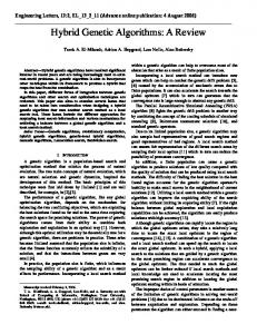
Snapshots of Ey on the plane y = 0 at t = 0.5 ns (left) by SEM with different interpolation orders for E and H and (right) by SEM with the same interpolation order for E and H. . . . . . . . . . . . . . . .
32
Eigenvalues of the cavity (left) by SEM with different interpolation orders for E and H and (right) by SEM with the same interpolation order for E and H. The dots denote the calculated eigenvalues by SEM schemes and the horizontal lines denote analytical solutions. .
32
Errors of four modes of the metallic cavity by non-spurious SEM with different interpolation orders. . . . . . . . . . . . . . . . . . . . . . .
33
An open-region time-domain scattering problem with a 10 cm × 10 cm × 10 cm dielectric cube (�r = 4) and a 10 cm × 10 cm × 10 cm PEC cube. . . . . . . . . . . . . . . . . . . . . . . . . . . . . . . . .
34
(left) Numerical results and (right) relative errors of time-varying received signals by the two SEM schemes. . . . . . . . . . . . . . . . .
35
4.10 (left) Numerical results and (right) relative errors of frequency components of received signals by the two SEM schemes. . . . . . . . . .
35
4.3 4.4 4.5
4.6
4.7 4.8
4.9
5.1 5.2 5.3
5.4
5.5
The dispersion curve of 1D mixed FEM system with common interpolation (linear basis function for both Ey and Hz ). . . . . . . . . . .
39
The first 12 eigenmodes by 1D mixed FEM system with common interpolation. . . . . . . . . . . . . . . . . . . . . . . . . . . . . . . . .
40
The dispersion schematic of 1D mixed FEM system with mixed interpolation (quadratic basis function for Ey and quadratic basis function for Hz ). . . . . . . . . . . . . . . . . . . . . . . . . . . . . . . . . . .
40
The dispersion curve of 1D mixed FEM system with mixed interpolation (quadratic basis function for Ey and linear basis function for Hz ). . . . . . . . . . . . . . . . . . . . . . . . . . . . . . . . . . . . .
42
The first 12 eigenmodes by 1D mixed FEM system with mixed interpolation. . . . . . . . . . . . . . . . . . . . . . . . . . . . . . . . . . .
42
xi
6.1
A schematic of the hybrid SETD/FETD discretization.
. . . . . . .
46
6.2
The shared area of two elements (a and b) with first order geometric transformation is a flat polygon, which is shown as the circled area in (c). . . . . . . . . . . . . . . . . . . . . . . . . . . . . . . . . . . . .
48
6.3
A ploy with N vertices (a) can be decomposed into N − 2 triangles (b). 48
6.4
A big system is divided into several smaller systems by hybrid SETD/FETD method. . . . . . . . . . . . . . . . . . . . . . . . . . . . . . . . . . . 51
7.1
A schematic of time stepping in IMEX-RK. . . . . . . . . . . . . . .
60
7.2
A schematic of coupled implicit subdomains in 1D array: (a) layered type (b) cascading type (c) mixed type. . . . . . . . . . . . . . . . .
64
A dielectric ring in a rectangular PEC cavity: a1 = 207.25 mm, a2 = 116.75 mm, b = 121 mm, c = 43 mm, r1 = 16.65 mm, r2 = 26.75 mm, h=39 mm [88]. . . . . . . . . . . . . . . . . . . . . . . . . . . . .
67
Different meshes for the resonant cavity loaded with dielectric ring: (a) The hybrid SETD/FETD method with 5 subdomains; (b) The non-spurious FETD method with one single domain. . . . . . . . . .
68
Measurement of the radiation of a chip in a reverberation chamber with two metal stirrers. The origin of coordinate as well as the chip is placed at the center of this chamber. . . . . . . . . . . . . . . . . .
69
The time-varying Ez components by an electric dipole placed at (0.5 m, 0.3 m, 0.1 m) calculated by the FDTD method and the hybrid SETD/FETD method. . . . . . . . . . . . . . . . . . . . . . . . . . .
70
The time-varying Ez components by an electric dipole placed at (0.5 m, -0.3 m, 0.1 m) calculated by the FDTD method and the hybrid SETD/FETD method. . . . . . . . . . . . . . . . . . . . . . . . . . .
70
The time-varying Ez components by an electric dipole placed at (-0.5 m, 0.3 m, 0.1 m) calculated by the FDTD method and the hybrid SETD/FETD method. . . . . . . . . . . . . . . . . . . . . . . . . . .
70
The time-varying Ez components by an electric dipole placed at (-0.5 m, -0.3 m, 0.1 m) calculated by the FDTD method and the hybrid SETD/FETD method. . . . . . . . . . . . . . . . . . . . . . . . . . .
71
8.8
An interconnect package with strips and vias. . . . . . . . . . . . . .
71
8.9
The interconnect package can be decomposed into several layers. . . .
72
8.1
8.2
8.3
8.4
8.5
8.6
8.7
xii
8.10 Four ports of the interconnect package. . . . . . . . . . . . . . . . . .
73
8.11 Calculated S-paremeters by HFSS, FDTD, and hybrid SETD/FETD.
73
8.12 A 5 × 5 patch antenna array. . . . . . . . . . . . . . . . . . . . . . . .
75
8.13 Patch antenna with thickness as 1 mm. . . . . . . . . . . . . . . . . .
75
8.14 Scattered voltage calculated by FDTD and hybrid SETD/FETD. . .
76
8.15 S-paramter calculated by FDTD and hybrid SETD/FETD. . . . . . .
76
8.16 Memory costs of the hybrid SETD/FETD method and the FDTD method for the antenna arrays with different numbers of cells. . . . .
78
xiii
List of Abbreviations and Symbols ADI
alternating-direction implicit method.
CFL
Courant-Friedrichs-Levy condition.
CN CT/LN DG
Crank-Nicolson method. constant tangential / linear normal basis functions. discontinuous Galerkin method.
DoF
degree of freedom.
ECT
enlarge cell technique.
EMC
electromagnetic compatibility.
EMI
electromagnetic interference.
ERK
explicit Runge-Kutta method.
ESDIRK FDTD FEM FETD FIT FVTD GLL GS IMEX-RK LT/QN
explicit singly diagonally implicit Runge-Kutta method. finite-difference time-domain method. finite element method. finite-element time-domain method. finite integration technique. finite-volume time-domain method. Gauss-Lobatto-Legendre polynomial. Gauss-Seidel iteration. implicit / explicit Runge-Kutta method. linear tangential / quadratic normal basis functions. xiv
MoM
method of moments.
PEC
perfect electric conductor.
PMC
perfect magnetic conductor.
PML
perfectly matched layer.
PSTD
pseudospectral time-domain method.
SETD
spectral-element time-domain method.
TLM
transmission line matrix method.
USC
uniformly stable conformal approach.
WETD
Whitney-element time-domain method.
xv
Acknowledgements At this moment of concluding my Ph.D. study in Duke University, I would like to express my sincere thanks to my advisor, Prof. Qing H. Liu, for introducing me to the fascinating area of time domain electromagnetic computation, for sharing me with his broad vision in research, and for continuously encouraging me in generating high quality outputs. I will cherish the three-and-a-half-year wonderful experience working with Prof. Liu all my life. I would like to thank my former advisors, Prof. Xicheng Wang and Prof. Wanxie Zhong from Dalian University of Technology, for introducing me to numerical analysis, computational mechanics, and computational electromagnetics. I would never have gone this far in science and research without their guidance and encouragement throughout my graduate study in China. I am grateful to Prof. William T. Joines, Prof. Tomoyuki Yoshie, Prof. John A. Trangenstein, and Prof. Anita T. Layton for being my committee member and giving me constructive suggestions. I will thank Prof. Jian-Guo Liu for serving my preliminary exam, and for the inspiring discussion about mixed finite element methods. It is always a great pleasure to exchange opinions with colleagues. I would express my deepest gratitude to Yueqing Huang, Luis Tobon, Yun Lin, Bao Zhu, Menqing Yuan, and Xi Rui from Duke University, Dr. Mei Chai and Dr. Jason A. Mix from Intel Corporation, Dr. Tiao Xiao, and Dr. Jun-Ho Lee from Wave Com-
xvi
putation Technologies, Inc., Dr. Chong Luo from Alpha Omega Electromagnetics, Dr. Zhenyu Huang from Qualcomm, and Dr. Zhonghai Guo from Apache Design Solutions for the countless help, stimulating discussions, valuable comments, and invaluable friendship. Last, but certainly not the least, I would like to thank my father Shihao Chen, my mother Shanhua Tan, my brother Yifu Chen, and my wife Shiqin Xu for their support, patience, and love. A few words are not enough to express my appreciation. This work is gratefully dedicated to them.
Thank you all, Jiefu Chen December 2010
xvii
1 Introduction
1.1 Problem Statement and Challenges The goal of our study is to develop an efficient algorithm for the transient analysis of multiscale electromagnetic problems. Realistic system level electromagnetic problems are often multiscale. Take the electronic packaging problem shown in Fig. 1.1 for example: electrically small structures with details much smaller than a typical wavelength, such as chip level components, and electrically large structures comparable to or larger than a typical wavelength, such as the space between chips and the enclosure, coexist in one system. To simulate this structure is a typical multiscale problem. Simulating the transient multiscale problems can be very challenging for conventional numerical methods. In terms of spatial discretization, conventional methods use a single mesh for the whole structure, thus a high discretization density required to capture the geometric characteristics of electrically fine structures will inevitably lead to a large number of wasted unknowns in the electrically coarse domains. This issue will become especially severe for orthogonal grids used by the
1
Figure 1.1: A multiscale problem contains electrically large structures, such as the space between motherboard and case, and electrically small structures, such as chip level components.
popular finite-difference time-domain (FDTD) method [1]-[2]. The finite-element time-domain (FETD) method [3]-[4] is more flexible in geometric modeling. However, this method requires inverting or factorizing system matrices, which can be prohibitively expensive when the number of unknowns becomes large. In terms of temporal integration, small cells in electrically fine domains will lead to extremely small time steps and an unaffordable number of calculations in time integration for explicit schemes, which have a maximum size of time step limited by the CourantFriedrichs-Levy (CFL) condition [5]. Implicit schemes can surpass the CFL limit. However, due to the large system matrices generated by conventional methods, it is almost impossible to employ implicit schemes to the whole structure for timestepping.
2
1.2 Previous Methods for Time Domain Electromagnetic Simulations In general, numerical methods for electromagnetic problems can be classified into two categories: the frequency domain methods and the time domain methods. Compared to the methods in frequency domain, the time domain methods are more suitable for simulations of transient electromagnetic fields and analysis of broadband properties of devices. A single simulation with a consequent Fourier transform post-processing is sufficient to characterize the electromagnetic behaviors of a system over a broad frequency band [6]-[7]. Among all the well established time domain methods, the FDTD method and the FETD method are intensively studied and widely used. Other time domain methods, such as the finite-volume time-domain (FVTD) method [8], the time domain method of moments (MoM) [9], the finite integration technique (FIT) [10], and the time domain transmission line matrix (TLM) method [11] are also used in computational electromagnetics. Every kind of method has its own advantages and disadvantages. It is impossible to generalize the superiority of a specific method over another unless a specific circumstance is designated. Based on the relationship to our study aim, in the following subsections we will focus our discussion on the FDTD method and the FETD method, and the hybrid methods based on these two time domain techniques. 1.2.1
The FDTD Method
The FDTD method is the most popular time domain method for computational electromagnetics. It is a direct method to Maxwell’s equations. Electric fields and magnetic fields are discretized on orthogonal grid points with a half cell offset both in space and time domain. In the basic FDTD scheme, the spatial discretization is based on hexahedrons named as the Yee’s cell [1], as shown in Fig. 1.2, and the
3
Figure 1.2: The Yee’s cell of the standard FDTD method: the electrical components are in the middle of the edges and the magnetic components are in the center of the faces. central difference method is employed for approximating both spatial and temporal derivatives. The FDTD method is a very simple time domain technique. It uses no linear algebra [2], so neither inverting system matrices nor solving matrix equations is required in the method. Besides, the accuracy and stability issues in the FDTD are carefully studied and well understood, making this method a robust tool for practical problems. Despite the above advantages, the requirement of orthogonal grids in the conventional FDTD method makes this method very inflexible in geometric modeling. As shown in Fig. 1.3, staircase error will arise when orthogonal grids are used to approximate geometries with curved shapes, thus great artificial reflections will be generated in the FDTD simulations [12]. The difficulty of geometric modeling will become more severe when the FDTD method is employed for multiscale electromagnetic simulations. To capture the geometric details of fine structures in a multiscale
4
Figure 1.3: Staircase error by the conventional FDTD method. system, a sufficient resolution is required in the electrically small region, which means an extremely high resolution in the electrically large region. Obviously, there will be a large number of grid points wasted in the electrically large domain. This unnecessary cost will greatly lower the overall computational efficiency of the FDTD method for multiscale simulations. The subgridding technique [13] can reduce the staircase error by using finer grid near the curved boundaries. However, this kind of method can not eliminate the staircase error from the root because the grid is still required to be orthogonal. The finer grid near curved boundaries will spoil the simple data structure of the conventional FDTD [14], thus greatly increase the computational complexity. What is worse, a general rule is still unavailable for the stability criterion of the subgridding method. The conformal FDTD (CFDTD) method [15]-[16] can eliminate the staircase error by using non-orthogonal grids. Because of the small irregular cells near the curved boundaries, the CFDTD method usually has a smaller stability criterion than the conventional one, and consequently it will lead to a larger number of time steps as 5
well as large dispersion errors. To address this drawback of the CFDTD method, several methods such as the uniformly stable conformal (USC) [17] approach and the enlarge cell technique (ECT) [18] are proposed to increase the CFL limit of the CFDTD method. Besides the spatial discretization, time stepping in multiscale electromagnetic simulations can also be a great challenge for the conventional FDTD method. The FDTD method requires the size of time step no larger than the stability criterion (the CFL limit), which is proportional to the grid size. Since the cell size in the electrically small region may be several orders shorter than a typical wave length, the stability condition will make the time step size several orders smaller than one period, e.g. millions or even more implementations of time stepping are required within one typical period, which will be unaffordable for the conventional FDTD method. Implicit time-stepping schemes can be used to help conventional FDTD method overcome the CFL limit. The alternating-direction implicit (ADI) [19] method and the Crank-Nicolson (CN) method [20] are two widely used implicit schemes to make the FDTD method unconditionally stable. However, implicit schemes require solving matrix equations at each time step, which will limit the FDTD method to problems with a moderate number of unknowns. The pseudo-spectral time-domain (PSTD) [21]-[22] method is a special type of higher order FDTD method. By using trigonometric functions or Chebyshev polynomials to approximate spatial derivatives, a very coarse sampling density is needed for this method to achieve spectral accuracy. This method is very efficient for electrically large problems with smooth internal media.
6
Figure 1.4: Tetrahedral, hexahedral and triangular prism element. 1.2.2
The FETD Method
The FETD method uses finite elements to achieve greater flexibility in geometric modeling. Based on the governing equations to be solved, this method can be divided into two types: one solves the second order vector wave equation with one variable, and the other directly solves Maxwell’s equations with two variables. The first FETD type can be viewed as the time domain version of the finite element method (FEM) [23] for computational electromagnetics, because both of them are based on the second order vector wave equation. As a result, the welldeveloped basis functions in the FEM can be easily adopted to the first FETD type. However, one of the major drawbacks of this type of FETD is the difficulty in the implementation of the time domain perfectly matched layer (PML) [24]-[25], which is used to truncate unbounded regions. This disadvantage greatly limits the application of this FETD type. It is more suitable to solve the open region problems by the second type of FETD method. A strongly well-posed PML [26] was proposed based on the Maxwell’s equations with two variables. It does not require any modification of the governing equations, thus makes it straightforward to incorporate the well-posed PML into the second FETD type. The vector elements [27]-[29] are employed in the FETD method for computa7
tional electromagnetics to facilitate the enforcement of boundary conditions as well as to eliminate the spurious modes [30]. The vector elements assign degrees of freedom (DoF) to the edges rather than to the nodes [23], and they use vector basis functions to make the continuity conditions automatically be satisfied across element interfaces. The tetrahedral, hexahedral, and triangular prism elements shown in Fig. 1.4 are three basic types of elements used in 3D FETD. In general, the tetrahedral element is most flexible in geometric modeling, the hexahedral element requires the smallest number of unknowns to reach a specific accuracy, and the triangular prism element is usually used in special situations such as discretizing layered structures. After spatial discretization by the vector elements, explicit and implicit schemes can be employed in the FETD method. Matrix equations are to be solved at each time steps for both the two schemes. The explicit scheme is conditionally stable, thus the size of time steps must be smaller than the stability criterion, which is determined by largest eigenvalue of the discretized FETD system. The system matrices by explicit schemes include only mass matrices, so it is very meaningful to make mass matrices diagonal or block-diagonal by introducing orthogonal basis functions [31]-[33]. This process can replace the step of solving matrix equations by directly inverting the mass matrices during time stepping. Implicit schemes for the FETD method are unconditionally stable, however, system matrices in implicit schemes include not only the mass matrices, but also the stiffness matrices, which cannot be diagonalized in any condition. The SETD method [34]-[38] is a special type of FETD method employing spectral element based on the Gauss-Lobatto-Legendre (GLL) sampling points. The mass matrices by the SETD method will be block diagonal, thus will make the inversion of mass matrices trivial. Besides, the construction of higher order element of the SETD is straightforward and systematic, so p-refinement is easily implemented and spectral accuracy can be obtained from the SETD method. 8
Figure 1.5: Conforming meshes (a) and non-conforming meshes (b) with different kinds of element in DG-FETD method. 1.2.3
The DG-FETD and DG-SETD Methods
The discontinuous Galerkin finite-element time-domain (DG-FETD) method [39][48] uses the technique of domain decomposition. The DG-FETD method divides a whole problem into several non-overlapping subdomains. As shown in Fig. 1.5, the types of elements in different subdomains can be the same or different, and the finite element meshes across interfaces between subdomains can be conforming or non-conforming. In the time-stepping of DG-FETD, each subdomain will be solved independently within one time step, and field correction will be enforced on the interfaces between subdomains via numerical fluxes [49]-[50]. The DG-FETD method is especially suitable for complex geometries and inhomogeneous materials, and it is also convenient for the implementation of parallel computations. The discontinuous Galerkin spectral-element time-domain (DG-SETD) method [51]-[55] can be viewed as a special type of DG-FETD. In this method the spectral elements with different interpolation degrees are employed in different subdomains to maximize the efficiency. The numerical error by this method will decrease exponentially with the increase of the interpolation degree, in other words, the DG-SETD method can achieve spectral accuracy.
9
Figure 1.6: A schematic mesh for the hybrid FDTD/FETD method. 1.2.4
The Hybrid FDTD/FETD Method
From the above discussion we can find that every numerical method has its own advantages and disadvantages. Under some specific circumstances one method may present superiority over others. Hybrid methods allow us divide a complex problem into several parts with different properties, and then choose a relatively “better” method for each part. Hybridizing the FDTD method with the FETD method [56]-[59] is a natural attempt because the former method is efficient in time stepping but inflexible in geometric modeling, while the latter one is less efficient but able to discretize arbitrary shapes. As shown in Fig. 1.6, in the hybrid FDTD/FETD method, the FETD method is used to model and solve the complex structure and its vicinity, while the FDTD method is used for other parts as well as the PML region. Although the hybrid FDTD/FETD method can combine the advantages of both methods and avoid their weakness, the hybridization of two different methods will bring new problems. The first issue is about the stability. The hybrid FDTD/FETD methods are usually instable, some are instantaneous instable, which is very severe 10
and completely unacceptable, and some others present late time instability, which is less severe but still will greatly decrease the accuracy of the hybrid method [7]. Worst of all, it is very difficult to find a general rule to predict and remedy the instability of a specific hybrid FDTD/FETD method, and this difficulty makes the hybrid FDTD/FETD method incapable to be a robust tool for practical problems. Mesh generation is another issue for the hybrid FDTD/FETD method. As shown in the Fig. 1.6, to make the hybrid FDTD/FETD method work, a special kind of “buffer mesh” is constructed near the interface between FDTD and FETD region, and both the FDTD grid and the FETD mesh are required to be conforming (or subgridding) to the buffer. Obviously, it is difficult to generate such mesh for very complex geometries, and this difficulty will greatly limit the application of the hybrid FDTD/FETD method. A quasi non-overlapping FDTD/FETD scheme is proposed based on the discontinuous Galerkin technique [60]. This scheme allows non-conforming meshes across the interface between FDTD domain and FETD domain, furthermore, it can divide the FETD domain into several subdomains. Numerical examples show that this new scheme is stable, and is more flexible in geometric modeling than previous hybrid FDTD/FETD methods.
1.3 Dissertation Overview This thesis is organized as follows. In Chapter 2 we discuss different forms of governing equations and corresponding FEM schemes for transient electromagnetic analysis; the mixed FEM based on Maxwell’s equations with E and H as variables is regarded as the best fit for the implementation of the hybrid SETD/FETD method. In Chapter 3 and Chapter 4 we discuss the construction of the non-spurious mixed FEM and SEM, respectively. In the hybrid SETD/FETD discretization of a multiscale structure the FEM is used to capture the geometry details of the electrically fine 11
part and the SEM is used to efficiently represent the electrically coarse part. We explain the origin of spurious modes in mixed FEM systems by dispersion analysis in Chapter 5, which can shed a light on how to construct non-spurious mixed FEM. We elaborate the spatial discretization of hybrid SETD/FETD method in Chapter 6. In Chapter 7 we discuss the time integration schemes of the hybrid SETD/FETD method for multiscale problems with different scenarios. Several examples are given in Chapter 8, which clearly demonstrate that the proposed hybrid SETD/FETD method is flexible and efficient in modeling multiscale problems. Finally, we list the original contributions for this topic, and give conclusions as well as suggestions for future work in chapter 9.
12
2 Governing Equations and Finite Element Discretization Schemes
The transient electromagnetic problems can be governed by different equations such as the first order Maxwell’s equations or the second order wave equations. Governing equations can be based on different variables, and these variables can be represented by different choices of basis functions. These choices of governing equations as well as basis functions will lead to several different FETD schemes for electromagnetic simulations. In this chapter we will discuss about these schemes and try to pick out a FETD scheme suitable for the further implementation of the hybrid SETD/FETD method.
2.1 EBHD Scheme Based on Maxwell’s Equations Maxwell’s equations depict all macroscopic electromagnetic phenomena. The differential form of Maxwell’s equations are ∂B + σm H + ∇ × E = −Ms ∂t
13
(2.1)
∂D + σe E − ∇ × H = −Js ∂t
(2.2)
∇·D=ρ
(2.3)
∇·B=0
(2.4)
where E and H are electric and magnetic field intensities; D and B are electric and magnetic flux densities; Js and Ms are applied electric and magnetic current densities; ρ is electrical charge density; �, µ, σe , and σm denote material’s permittivity, permeability, electric conductivity, and magnetic conductivity, respectively. In the EBHD scheme, E and H are discretized by the curl-conforming basis function; D and B are discretized by the div-conforming basis functions. Numerical experiments reveal that the EBHD scheme has poor performance due to the presence of spurious modes [61]. This issue makes the EBHD scheme unsuitable for time domain simulation with sources.
2.2 EB Scheme Based on Maxwell’s Equations The four variables E, H, D, and B are not independent variables. The constitutive relations among them are D = �E
(2.5)
B = µH
(2.6)
where � and µ denote the permittivity and permeability, respectively. These parameters are space-varying quantities for inhomogeneous media, and they are scalars for isotropic media and tensors for anisotropic media. The EB scheme is based on Maxwell’s equations with two variables E and B, i.e. ∂B σm + B + ∇ × E = −Ms ∂t µ 14
(2.7)
�
∂E 1 + σe E − ∇ × B = −Js ∂t µ
(2.8)
Curl-conforming and div-conforming basis functions are employed to discretized variables E and B, respectively [62]. This scheme is free of spurious modes, which is essential for solving driven electromagnetic problems. However, because the EB scheme represents variable B by div-conforming basis functions, which provide normal continuity, not the tangential continuity on an interface; while the numerical flux [50] requires the tangential components of E and H to make the DG-FETD method work for multiple subdomains. This issue makes the EB scheme unsuitable for further implementation of the DG-FETD method or the hybrid SETD/FETD method.
2.3 Vector Wave Equation Scheme With the aid of constitutive relations and by eliminating H from Maxwell’s equations, the vector wave equations based on one variable E can be obtained as 1 ∇ × ( ∇ × E) − ω 2 �E = −jωJ µ
(2.9)
The vector wave equation scheme is also known as the Whitney-element timedomain (WETD) scheme [63]. It discretizes the only variable E in the above equations by the curl-conforming basis functions. This FETD scheme can be viewed as the time domain version of the FEM [23] for computational electromagnetics because both of these two methods are based on the second order vector wave equation. As a result, the well-developed non-spurious basis functions in the FEM can be easily adapted to this scheme. However, this FETD scheme has difficulty in implementation of the PML [24]-[25], which is extensively used to truncate unbounded regions. What is worse, because this FETD scheme is based on one variable but the numerical fluxes are based on both E and H on the interface, the implementation of the 15
DG-FETD method or the hybrid SETD/FETD mehtod will be very inconvenient for this vector wave equation based FETD scheme.
2.4 EH Scheme Based on Maxwell’s Equations Transient electromagnetic phenomena can also be simulated by solving the two coupled first order equations with variables E and H ∂E + σe E − ∇ × H = −Js ∂t
(2.10)
∂H + σm H + ∇ × E = −Ms ∂t
(2.11)
�
µ
The EH scheme uses the curl-conforming basis functions to represent E and H, thus the tangential continuities of both two variables on interface are preserved. This property makes the evaluation of numerical flux straightforward in the EH scheme. Furthermore, since this scheme is based on two variables, it is very convenient to implement PML for open-region problems. The above two benefits of the EH scheme make it a potentially promising scheme for the implementation of the DG-FETD method and the hybrid SETD/FETD method. Beside the above advantages of EH scheme based on Maxwell’s equations, the appearance of spurious modes can be a serious issue for this scheme. It is well-known that the curl-conforming basis functions can suppress the spurious modes when they are used to solve the second order vector wave equations. However, for EH scheme based on the Maxwell’s equations, spurious modes may still be stimulated even such curl-conforming basis functions are utilized to discretize both E and H [64]-[69]. In the following chapters we will discuss this issue of the EH scheme, also we will discuss how to solve this issue and make this scheme suitable for further implementation of the hybrid SETD/FETD method by constructing a non-spurious FETD scheme as well as a non-spurious SETD scheme. 16
3 Non-Spurious Mixed Finite Element for Maxwell’s Equations
In this chapter we will discuss about how to construct non-spurious mixed finite element for solving time-dependent Maxwell’s equations based on two variable E and H [64]. In the hybrid SETD/FETD method, the finite element part is employed to discretize electrically fine structures with complex details. To maximize FETD’s flexibility in geometric modeling, tetrahedra with lower interpolation degree are chosen to construct non-spurious mixed finite elements.
3.1 Mixed-Order Curl-Conforming Vector Basis Functions As discussed in the previous chapter, we found the EH scheme base on Maxwell’s equations is most suitable for implementation of the DG-FETD method and the hybrid SETD/FETD method. Mixed-order curl-conforming vector basis functions are used in this scheme due to the convenience of constructing time domain PML as well as applying boundary / interface conditions. Two types of lower order vector basis functions: the constant tangential / linear normal (CT/LN), and the linear
17
Figure 3.1: A tetrahedral CT/LN element, the numbers in circles and with arrows denote the labels of nodes and basis functions, respectively. tangential / quadratic normal (LT/QN) mixed-order curl-conforming vector basis functions are employed to build the non-spurious mixed finite element. 3.1.1
The Tetrahedral CT/LN Vector Element
The CT/LN element is the simplest form of the mixed-order curl-conforming vector element [65], also known as the Whitney element [66], or the N´ed´elec element [27]. The construction of CT/LN element is based on the scalar basis functions for the linear scalar tetrahedral element . A scalar field f within a linear tetrahrdon as shown in Fig. 3.2 can be approximated as
f (x, y, z) =
4 X
Lj (x, y, z)fj
(3.1)
j=1
where fj denotes the field value at the j-th node. The linear scalar interpolation functions Lj (x, y, z) are given by Lj (x, y, z) =
1 (aj + bj x + cj y + cj z) 6Ve 18
(3.2)
where Ve denotes the volume of the element. Detailed expressions of Ve and coefficients aj , bj , cj , dj are referred to [23] and will not be elaborated here. The CT/LN vector element assigns degrees of freedom to the edges, not the nodes, thus it is also named as edge element [67]. The mixed-order curl-conforming vector basis functions associated with the six edges of the CT/LN element are list in Tab. 3.1 [23]. It is easy to prove that N can provide the continuous tangential components, while allow discontinuous normal components across an interface shared by two adjacent element. These properties make it very suitable in representing electrical and magnetic fields with inhomogeneous media. Table 3.1: Basis functions of the CT/LN element edge 1 2 3 4 5 6
3.1.2
starting node 1 1 1 2 4 3
ending node 2 3 4 3 2 4
basis function L1 ∇L2 − L2 ∇L1 L1 ∇L3 − L3 ∇L1 L1 ∇L4 − L4 ∇L1 L2 ∇L3 − L3 ∇L2 L4 ∇L2 − L2 ∇L4 L3 ∇L4 − L4 ∇L3
The Tetrahedral LT/QN Vector Element
The LT/QN element is also a type of mixed-order curl-conforming vector element, but with one order higher than the CT/LN element. A LT/QN element contains ten nodes and 12 edges. Each edge is associated with one vector basis functions providing linear tangential components, which are shown in Tab. 3.2, and each face is associated with two vector basis functions providing quadratic normal components, as shown in 3.3.
19
Figure 3.2: A tetrahedral LT/QN element, the numbers in circles and with arrows denote the labels of nodes and basis functions, respectively. Table 3.2: Edge-based basis functions of the LT/QN element edge 1 2 3 4 5 6 7 8 9 10 11 12
starting node 1 2 1 3 1 4 2 3 2 4 3 4
ending node 5 5 7 7 8 8 6 6 9 9 10 10
basis function L1 ∇L2 L2 ∇L1 L1 ∇L3 L3 ∇L1 L1 ∇L4 L4 ∇L1 L2 ∇L3 L3 ∇L2 L2 ∇L4 L4 ∇L2 L3 ∇L4 L4 ∇L3
3.2 Non-Spurious Mixed Finite Element Spurious mode can be an issue for the FETD scheme based on Maxwell’s equations with variables E and H. Merely representing both E and H by vector basis function cannot guarantee the FETD scheme is free of spurious modes [68]. Based on 20
Table 3.3: Face-based basis functions of the LT/QN element face 1 1 2 2 3 3 4 4
associated 2 3 2 3 1 3 1 3 1 2 1 2 1 2 1 2
nodes 4 4 4 4 4 4 3 3
basis function L2 L3 ∇L4 - L2 L4 ∇L3 L3 L4 ∇L2 - L2 L4 ∇L3 L1 L3 ∇L4 - L1 L4 ∇L3 L3 L4 ∇L1 - L2 L4 ∇L3 L1 L2 ∇L4 - L1 L4 ∇L2 L2 L4 ∇L1 - L1 L4 ∇L2 L1 L2 ∇L3 - L1 L3 ∇L2 L2 L3 ∇L1 - L1 L3 ∇L2
numerical experiments and dispersion analysis, we find the following two conditions can guarantee a non-spurious vector FETD scheme for Maxwell’s equations: 1) Choose the first family of the N´ed´elec elements, i.e. the curl-conforming edge element to represent both E and H in Maxwell’s equations. The vector basis functions can greatly facilitate the imposition of boundary conditions as well as the implementation of numerical fluxes on the interfaces; 2) Choose different interpolation degrees for E and H. For example, the combination of the LT/QN element for E and the CT/LN element for H (or vice versa) is a lower order non-spurious FETD scheme. Higher order non-spurious tetrahedral elements as well as non-spurious hexahedral elements can also be constructed following the same idea.
3.3 Galerkin’s Weak Form and Discretized System Denote Ne and Nh as basis functions for E and H, respectively. The Galerkin’s weak forms of Maxwell’s equations are �
Z V
Z V
� ∂E Φ· � + σe E − ∇ × H + Js dV = 0 ∂t
� ∂H Ψ· µ + σm H + ∇ × E + Ms dV = 0 ∂t
(3.3)
�
21
(3.4)
The discretized system of equations by the FETD scheme are de = Cee e + Keh h + j dt
(3.5)
dh = Khe e + Chh h + m dt
(3.6)
Mee
Mhh
where e and h are vectors of the discretized electric and magnetic fields. j and m are vectors of the discretized excitations. Mee and Mhh are the mass matrices, Cee and Chh are the damping matrices, Keh and Khe are the stiffness matrices. Z �Φk · Φl dV
(3.7)
µΨk · Ψl dV
(3.8)
σe Φk · Φl dV
(3.9)
σm Ψk · Ψl dV
(3.10)
Φk · ∇ × Ψl dV
(3.11)
(Mee )kl = V
Z (Mhh )kl = V
Z (Cee )kl = − V
Z (Chh )kl = − V
Z (Keh )kl = V
Z (Khe )kl = −
Ψk · ∇ × Φl dV
(3.12)
V
Z (j)k = −
Φk · Js dV V
22
(3.13)
Figure 3.3: A 10 cm × 8 cm × 2 cm PEC cavity divided into two non-orthogonal subdomains with non-conforming meshes on the two interfaces. Z Ψk · Ms dV
(m)k = −
(3.14)
V
Several time stepping schemes such as the leap-frog scheme, the Crank-Nicolson (CN) method, the Runge-Kutta (RK) method etc. can be applied to carry out time integration for the above system of equations. The appearance of spurious modes can be easily recognized from time integration results as well as frequency components with Fourier analysis as post processing.
3.4 Numerical Results Consider a 10 cm × 8 cm × 2 cm metallic cavity filled with air centered at the origin in Fig. 3.3. This cavity is divided into two non-orthogonal subdomains with non-conforming meshes on interfaces. A Blackman-Harris window pulse [?] with characteristic frequency 3.15 GHz is placed on a z-direction point dipole in subdomain 2 at (3.0, 2.0, -0.8) cm as the source, and a z-direction point dipole is placed in the subdomain 1 at (-1.8, -0.8, 0) cm as the receiver. We carry out time integration for 8000 steps by the proposed FETD scheme with ∆t = 5 ps. Fig. 3.4 shows the analytical results of resonant frequencies of the cavity as well as the numerical results by the proposed non-spurious FETD, which is 23
−6
−6
10 spectrum magnitude
spectrum magnitude
10
−8
10
−10
10
2
DG−FETD scheme 1 analytical results 3 4 frequency (Hz)
5
−8
10
−10
10
2
9
DG−FETD scheme 2 analytical results 3 4 frequency (Hz)
5 9
x 10 x 10 Figure 3.4: Resonant frequencies of the cavity by applying FFT to the timevarying received signal. DG-FETD scheme 1 chooses LT/QN and CT/LN elements to discretize E and H respectively (left); DG-FETD scheme 2 uses LT/QN elements to represent E and H simultaneously (right).
denoted as FETD scheme 1. For the aim of comparison we also plot the numerical results by FETD scheme 2, which uses a same type of edge element (LT/QN element in this case) to represent both E and H. From this figure we can clearly see that choosing edge elements with different interpolation degrees for different variables in Maxwell’s equations will suppress spurious modes, otherwise numerous spurious solutions will be generated to corrupt the correct results.
24
4 Non-Spurious Mixed Spectral Element for Maxwell’s Equations
In this chapter we will discuss about how to construct non-spurious mixed spectral element method (SEM) for solving time-dependent Maxwell’s equations based on two variable E and H [69]. In the hybrid SETD/FETD method, the SETD part is based on non-spurious SEM and is employed to discretize electrically coarse structures. Hexahedral elements with higher interpolation degree are used in SETD subdomains to achieve high accuracy and efficiency. There are two types of SEM [34]-[38] for computational electromagnetics: One is based on the second order wave equation and the other is based on the first order Maxwell’s equations. As to the aim of implementation of the hybrid SETD/FETD method, the second version of SEM is superior to the first one because the numerical fluxes such as the Riemann solver [50], which are the critical parts used in DG to communicate and correct fields between different subdomains, are defined by tangential components of E and H on the interfaces between subdomains. To construct a robust hybrid SETD/FETD method for electromagnetic problems, a non-spurious
25
SEM scheme based on variables E and H for the first order Maxwell’s equations is in demand. While it is well-known that the employment of mixed-order curl-conforming vector basis function can make a SEM scheme based on the second order wave equation free of spurious modes [27], the same technique, viz. merely using vector basis functions for both E and H cannot guarantee a non-spurious SEM scheme for the first order Maxwell’s equations [68]. Based on our numerical experiments, we find mixed interpolation is required to construct non-spurious vector spectral element schemes for Maxwell’s equations, i.e. the interpolation degree of vector basic functions for E must be different from that for H.
4.1 Non-spurious Mixed Spectral Element We use the mixed-order curl-conforming vector spectral elements [70] to discretize ˆ (M ) as the vector basis function for both E and H in Maxwell’s equations. Denote Φ E with M -th interpolation degree, we have −1) (M ) (M ) ξ ˆ (M ) ˆ (M Φmnp = ξφ (ξ)φn (η)φp (ζ) m (M ) (M −1) (M ) η ˆ (M ) Φmnp = ηˆφm (ξ)φn (η)φp (ζ) ) (M ) (M −1) ζ ˆ (M ) ˆ (M Φmnp = ζφ (ζ) m (ξ)φn (η)φp
(4.1)
where ) φ(M m (ξ) =
−(1 − ξ 2 )L0M (ξ) , m = 0, ..., M M (M + 1)LM (ξm )(ξ − ξm )
(4.2)
2 LM (ξ) is the Legendre polynomial of degree of M . ξm is chosen as (1 − ξm )L0M (ξm ) = (M )
(M )
0. φn (η) and φp (ζ) are functions of η and ζ, respectively, and they have similar (M )
formulation as φm (ξ). As shown in Fig. 4.1, ξ, η, and ζ are the coordinates in the reference domain [−1, 1] × [−1, 1] × [−1, 1], which is a standard cube mapped from 26
ζ
z
η
y ξ
x
(a) (b) Figure 4.1: A curved hexahedron in the physical domain (a) will be mapped into a standard cube in the reference domain (b) by geometric transformation. Second order geometric mapping is shown in this schematic [71].
Figure 4.2: A non-spurious SEM scheme for the Maxwell’s equations: (left) second order element for E and (right) first order element for H. ˆ ηˆ, and ζˆ denote the unit an arbitrary curved hexahedron in the physical domain. ξ, vector along the corresponding direction. The vector basis functions for H are almost the same with the basis functions for ˆ (N ) with N -th interpolation degree for instance E. Take Ψ −1) (N ) (N ) ξ ˆ (N ) ˆ (N Ψmnp = ξφ (ξ)φn (η)φp (ζ) m (N ) (N −1) (N ) η ˆ (N ) Ψmnp = ηˆφm (ξ)φn (η)φp (ζ) ) (N ) (N −1) ζ ˆ (N ) ˆ (N Ψmnp = ζφ (ζ) m (ξ)φn (η)φp
(4.3)
All arguments in (4.3) have the same meanings with those in (4.1) and (4.2). ˆ (M ) and Ψ ˆ (N ) are vector-based basis functions, spurious modes Although both Φ ˆ (M ) is will still be generated under distorted meshes if the interpolation order for Φ 27
ˆ (N ) [72]. Based on our numerical experiments, we set as the same with that for Ψ found that there is one more condition to be satisfied to construct a non-spurious vector spectral element method for Maxwell’s equations: The interpolation degree ˆ (M ) must be different from that of Ψ ˆ (N ) , i. e. M 6= N . A non-spurious SEM of Φ scheme for Maxwell’s equations is shown in Fig. 4.2.
4.2 Galerkin’s Weak Form and Discretized System The Galerkin’s weak forms of Maxwell’s equations are Z Ne X dej j=1
dt
1
−1
=
1
Z
−1
Nh X
−
1
Z
1
Z
� � ˆT ∇ ˆ k dξdηdζ ˆ Φ × Ψ i
−1
−1
−1
1
1
1
Z
Z
Z
ˆ T J−T σe J−1 Φ ˆ j |J|dξdηdζ Φ i
ej −1
1
1
Z
hk
j=1
Z
ˆ T J−T �J−1 Φ ˆ j |J|dξdηdζ Φ i
−1
k=1 Ne X
1
Z
Z
1
−1 1
Z
ˆ T J−T Js |J|dξdηdζ Φ i
− −1
−1
−1
−1
i = 1, 2, · · · , Ne
Z Nh X dhk k=1
dt
1
Z
−1
=−
1
Ne X
−
Z
1
1
−1
Z
1
Z
1
Z
−1
−1
Z
1
1
Z
1
Z
−1
−1
� � ˆ j dξdηdζ ˆT ∇ ˆ Ψ × Φ l
−1 1
hk
ˆ T J−T σm J−1 Ψ ˆ j |J|dξdηdζ Ψ i
−1
1
− −1
Z
ej
k=1
Z
ˆ T J−T µJ−1 Ψ ˆ k |J|dξdηdζ Ψ l
−1
j=1 Nh X
1
Z
−1
(4.4)
ˆ T J−T Ms |J|dξdηdζ Ψ i
−1
l = 1, 2, · · · , Nh 28
(4.5)
where Ne and Nh denote the numbers of unknowns of E and H. ej and hk are ˆ j and Ψ ˆ k , respectively. coefficients for Φ By assembling all spectral elements we will obtain the discretized system of equations de = Cee e + Keh h + j dt
(4.6)
dh = Khe e + Chh h + m dt
(4.7)
Mee and Mhh
where e and h are vectors of the discretized electric and magnetic fields. j and m are vectors of the discretized excitations. respectively. The detailed expressions for the above system matrices Mee , Mhh , Cee , Chh , Keh , and Khe can be referred to (3.7) (3.12). The formulation (4.6) and (4.7) are systems of ordinary differential equations in the time domain. Several time stepping algorithms, such as the leap-frog scheme and the Runge-Kutta method can be utilized to solve them. Besides, with the time convention d/dt → jω, we can easily transform (4.6) and (4.7) from the time domain into the frequency domain, in which the spurious modes are easier to be distinguished in the form of eigenmodes, and the spectral accuracy of the proposed method itself is more convenient to be demonstrated because the numerical errors due to time integration will not be introduced into SEM in the frequency domain. In the next section we will show some results by this non-spurious SEM in both time domain and frequency domain.
4.3 Numerical Results We first consider a 1 cm × 0.5 cm × 0.75 cm metallic cavity filled with air centered at the origin of coordinates. In order to show the spurious modes by other basis 29
Figure 4.3: A distorted mesh for a metallic cavity, which has a dimension of 1 cm × 0.5 cm × 0.75 cm and is filled with vacuum. functions, we use a distorted hexahedral mesh to discretize this cavity, which is shown in Fig. 4.3. We choose two different SEM schemes to solve the this problem: scheme 1 is SEM with different interpolation orders for E and H (M = 5, N = 4 in this case), and scheme 2 is SEM with the same interpolation order for E and H (M = 5, N = 5 in this case). We place a dipole with polarization −0.62ˆ x + 0.62ˆ y + 0.47ˆ z at (-0.014, -0.236, 0.011) cm, and give the first derivative of the Blackman-Harris window pulse [?] with characteristic frequency as 9.4 GHz on the dipole, so only the dominant mode can be stimulated. We use these two SEM schemes to discretize this problem and use the 4th order Runge-Kutta method for time stepping (with ∆t = 0.5 ps). Fig. 4.4 shows the time-varying Ey at (0.174, 0.239, 0.174) cm and the frequency components by the two SEM schemes. From which we find that only one mode is stimulated by scheme 1 and the corresponding time-varying results by scheme 1 agree well with the reference, while scheme 2 will stimulate a lot of spurious mode and lead the time domain results deviating greatly from the reference. Fig. 4.5 shows the snapshots of Ey on the plane y = 0 at 1000-th time step (t = 0.5 ns). We observe that the field pattern by scheme 1 is consistent with the dominant mode (TE101 ), while the results
30
y
normalized E (V/m)
reference SEM scheme 1 SEM scheme 2
2 1 0 −1 1
1.1
1.2
1.3
1.4
1.5
1.6
time (s)
−9
x 10
x 10
TE101
|FFT(Ey)|
1
1.7 −9
reference SEM scheme 1 SEM scheme 2
0.8 0.6 0.4 0.2 0 0
1
2
3
frequency (Hz)
4
5
6 10
x 10
Figure 4.4: (upper) Time-varying Ey on (0.174, 0.239, 0.174) cm by two SEM schemes and (lower) corresponding frequency components after FFT.
by scheme 2 are contaminated by spurious modes. Then we use these two SEM schemes to solve the eigenvalue problem of this cavity in frequency domain. Fig. 4.6 shows the calculated eigenvalues by the two SEM schemes as well as analytical solutions, from which we find that the results by scheme 1 agree very well with analytical solutions, while scheme 2 generates many spurious eigenvalues between every two adjacent analytical eigenvalues. In Fig. 4.7 we plot the errors of four modes (TE101 , TM110 , TE011 , and TE111 ) of this cavity by the non-spurious SEM with different interpolation orders of basis functions (M = 1, 2, · · · , 7, N = M + 1), from which we observe that the errors of all the four modes decrease exponentially with the increase of interpolation order, i. e. the proposed non-spurious spectral element method can achieve spectral accuracy.
31
Figure 4.5: Snapshots of Ey on the plane y = 0 at t = 0.5 ns (left) by SEM with different interpolation orders for E and H and (right) by SEM with the same interpolation order for E and H.
14
14
12
12
10
10
K0 (cm−1)
16
K0 (cm−1)
16
8
8
6
6
4
4
2
2
0
10
20
30
40
50
0
100
200
300
400
order of eigenvalue (scheme 2)
order of eigenvalue (scheme 1)
Figure 4.6: Eigenvalues of the cavity (left) by SEM with different interpolation orders for E and H and (right) by SEM with the same interpolation order for E and H. The dots denote the calculated eigenvalues by SEM schemes and the horizontal lines denote analytical solutions.
32
0
relative error
10
−5
10
TE101 TM110 TE011 TE111
−10
10
1
2 3 4 5 6 interpolation order of M (N=M+1)
7
Figure 4.7: Errors of four modes of the metallic cavity by non-spurious SEM with different interpolation orders.
The second example is an open-region time-domain scattering problem with one dielectric cube and one PEC cube, both with a side length of 10 cm. The dielectric cube with �r = 4 is centered at the origin, while the PEC cube is centered at (20, 20, 20) cm. The background medium in this example is air. A z−direction electric dipole is placed at the origin as the source, with the first derivative of the BlackmanHarris Window of characteristic frequency 1.55 GHz (i.e., with a pulse duration of 1 ns) as the time function. Another z−direction dipole is placed at (11, 11, 11) cm as a receiver. A schematic of the second example is shown in Fig. 4.8. Two SEM schemes are chosen for the time-domain simulation of this problem. Scheme 1 is the SEM with different interpolation orders for E and H (M = 2, N = 1 in this case), and scheme 2 is the SEM with the same interpolation order for E and H (M = 2, N = 2 in this case). Since analytical solution is not available for this problem, numerical results by the finite-difference time-domain method enhanced by the enlarged cell technique in a commercial software, Wavenology EM [73], under a relatively dense grid are used as the reference. Fig. 4.9 shows the received timevarying signals by the two SEM schemes as well as the reference result and the relative 33
Figure 4.8: An open-region time-domain scattering problem with a 10 cm × 10 cm × 10 cm dielectric cube (�r = 4) and a 10 cm × 10 cm × 10 cm PEC cube.
errors. From these plots we observe that the result by SEM scheme 1 agrees well with the reference, while the result by SEM scheme 2 does not. Fig. 4.10 shows the comparison between numerical results and the reference in the frequency domain and the relative errors. From these figures we clearly observe good agreement between the result by SEM scheme 1 and the reference, while we find some spurious peaks in the low frequency regime from the result by SEM scheme 2. Based on these two figures, we can conclude that for an open-region problem, the SEM with different interpolation orders for E and H is a spurious-free scheme; however, the SEM scheme with same interpolation order for both E and H will generate spurious modes, and these spurious modes will contaminate time-domain and frequency-domain results.
34
1 reference SEM scheme 1 SEM scheme 2
0.1
SEM scheme 1 SEM scheme 2
0.8 relative error
received signals (V/m)
0.2
0 −0.1
0.6 0.4 0.2 0
−0.2 0
0.5 time (s)
1
0
0.5 time (s)
−8
x 10
1 −8
x 10
Figure 4.9: (left) Numerical results and (right) relative errors of time-varying received signals by the two SEM schemes.
−11
x 10
1 reference SEM scheme 1 SEM scheme 2
6 4 2 0 0
SEM scheme 1 SEM scheme 2
0.8 relative error
spectrum magnitude
8
0.6 0.4 0.2 0
1
2 3 frequency (Hz)
4
5
0
9
x 10
1
2 3 frequency (Hz)
4
5 9
x 10
Figure 4.10: (left) Numerical results and (right) relative errors of frequency components of received signals by the two SEM schemes.
35
5 Dispersion Analysis for Mixed Finite Element Method
In the previous two chapters we proposed the non-spurious mixed FEM and nonspurious mixed SEM for Maxwell’s equations with two variable E and H. Based on numerical tests we found mixed interpolation, i.e. different interpolation degrees for different variables is one necessary conditions for a non-spurious mixed FEM scheme. In this chapter we will apply dispersion analysis [74]-[76] to several mixed FEM systems. Dispersion curve can clearly predict that whether or not spurious modes will appear for a specific mixed FEM system.
5.1 Mixed FEM System with Common Interpolation We start the dispersion analysis from the simple 1D TEz case in a unbounded, lossless, and homogeneous space µ
∂Hz ∂Ey + =0 ∂t ∂x
(5.1)
�
∂Ey ∂Hz + =0 ∂t ∂x
(5.2)
36
Take φ(x) and ψ(x) as basis functions for Ey (x) and Hz (x)
Ey (x) =
N X
En φj (x)
(5.3)
Hm ψj (x)
(5.4)
n=1
Hz (x) =
M X m=1
where N and M denote the total DoF for Ey and Hz , respectively. The discretized weak form of Maxwell’s equations will be
jω�
N X
Z Ep
φq φp dx +
Z Hp
φq
p=1
p=1
N X
M X
dψp dx = 0, dx
Z M X dφp Hp ψq ψp dx = 0, ψq dx + jωµ dx p=1
Z Ep
p=1
q = 1, 2, · · · , N
(5.5)
q = 1, 2, · · · , M
(5.6)
Assume the field values at the p-th node can be expanded as �
Ep Ep
�
�
E H
=
�
ejkxp
(5.7)
where k is the wavenumber. For a uniform FEM mesh with linear common interpolation, i.e. using linear basis function for both φ(x) and ψ(x), we will have N X
Z Ep
Z
xq
φq φp dx = Eq−1
Z
xq−1
p=1
Z
xq+1
φq φq−1 dx + Eq
φq φq dx xq−1
xq+1
+Eq+1
φq φq+1 dx = Eejkxq (cos(kd) + 2)d/3
(5.8)
xq
N X p=1
Z Hp
dψp φq dx = Hq−1 dx
Z
xq
dψq−1 φq dx + Hq dx xq−1 37
Z
xq+1
φq xq−1
dψq dx dx
Z
xq+1
φq
+Hq+1 xq
dψq+1 dx = Hejkxq j sin(kd) dx
(5.9)
where d is the elemental length of the 1D uniform mesh. Based on (5.8) and (5.9) we can obtain a matrix equation �
ω� (cos(kd) 3
+ 2)d sin(kd)
sin(kd) ωµ (cos(kd) + 2)d 3
��
E H
�
� =
0 0
� (5.10)
and consequently the dispersion relation 1 3 sin(kd) ω= d 2 + cos(kd)
r
1 µ�
(5.11)
From (5.11) we know that this 1D mixed FEM system with linear common interpolation will have numerical values of wavenumber as ω 1 3 sin(kd) k˜ = = c d 2 + cos(kd)
(5.12)
The dispersion curves of the 1D mixed FEM system with linear common interpolation as well as that of the accurate system are shown in Fig. 5.1. From this figure we observe that dispersion curve by the mixed FEM system agrees well with the real one when the value of kd is small (i.e. high sampling density), however, the numerical dispersion curve will drop to 0 when kd = π (i.e. d equals to a half wavelength, the Nyquist limit).This non-monotonic behavior can predict that the mixed FEM system with common interpolation will generate spurious modes. Numerical results can verify the prediction based on dispersion analysis. Consider a 1D periodic problem with unit length. The whole computational domain is discretized by a uniform FEM mesh with 100 elements. The first 12 eigenvalues and eigenmodes are shown in Fig. 5.2 and Tab. 5.1, respectively. From them we observe that three out from every four consecutive numerical solutions agree well with the 38
numerical value of kd
3 accurate system mixed FEM system
2.5 2 1.5 1 0.5 0
0
1 2 real value of kd
3
Figure 5.1: The dispersion curve of 1D mixed FEM system with common interpolation (linear basis function for both Ey and Hz ).
analytical ones, and the other one is spurious modes since it highly oscillates spatially but has relatively small k value. All these numerical behaviors are consistent with this mixed FEM system’s dispersion curve shown in Fig. 5.1. Table 5.1: First 12 eigenvalues by 1D mixed FEM system with common interpolation, dashed lines denote non-physical modes without correspondence in analytical solution Mode 1 2 3 4 5 6 7 8 9 10 11 12
numerical k (m−1 ) 0.0000 6.2832 12.5664 18.8001 18.8494 25.1322 31.4142 37.3058 37.6948 43.9729 50.2471 55.2360
39
analytical k (m−1 ) --6.2832 12.5664 --18.8496 25.1327 31.4159 --37.6991 43.9823 50.2655 ---
−0.5
0
0.5 x
1
0
y
−0.5 −1
0
0.5 x
−0.5 −1
1
0
0.5 x
0 −0.5 −1
1
1
1
0.5
0.5
−0.5 −1
0
0.5 x
−0.5 −1
1
0
y
0
y
0
Ey (mode 8 )
1 0.5
E (mode 7 )
1 0.5
E (mode 6 )
0
0.5 x
−0.5 −1
1
0
0.5 x
1
1
1
0.5
0.5
0.5
−1
0
0.5 x
1
0
y
0
y
0
Ey (mode 12 )
1
−0.5
−0.5 −1
0
0.5 x
1
−0.5 −1
0
0.5 x
1
0.5 x
1
0
0.5 x
1
0
0.5 x
1
−0.5 −1
1
0
0
0.5
E (mode 11 )
Ey (mode 5 )
−1
Ey (mode 9 )
0
y
0
Ey (mode 4 )
1 0.5
E (mode 3 )
1 0.5
E (mode 2 )
1 0.5
E (mode 10 )
Ey (mode 1 )
1 0.5
0 −0.5 −1
Figure 5.2: The first 12 eigenmodes by 1D mixed FEM system with common interpolation.
Figure 5.3: The dispersion schematic of 1D mixed FEM system with mixed interpolation (quadratic basis function for Ey and quadratic basis function for Hz ).
5.2 Mixed FEM System with Mixed Interpolation As we showed in the previous chapters, changing the mixed FEM scheme from common interpolation to mixed interpolation can eliminate spurious modes. Here we consider a simple scheme of mixed interpolation: using quadratic basis function and linear basis function to represent Ey and Hz , respectively. The 1D FEM mesh is still assume as uniform with discretization interval d. To perform dispersion analysis for 1D mixed FEM system as shown in 5.3, the
40
Ampere’s law will be discretized at the (i − 1/2)−th, i−th, and (i + 1/2)−th point.
jω�d (Ei−1 15
+ 8Ei−1/2 + Ei ) + 32 (−Hi−1 + Hi ) = 0
jω�d (−Ei−1 30 jω�d (Ei 15
+ 2Ei−1/2 + 8Ei + 2Ei+1/2 − Ei+1 ) + 61 (−Hi−1 + Hi+1 ) = 0 (5.13)
+ 8Ei+1/2 + Ei+1 ) + 32 (−Hi + Hi+1 ) = 0
And the Faraday’s law only needs to be discretized at the i-th point jωµd 1 (−Ei−1 − 4Ei−1/2 + 4Ei+1/2 + Ei+1 ) + (Hi−1 + 4Hi + Hi+1 ) = 0 6 6
(5.14)
With the same assumption in (5.7) and elimination of Ei−1/2 and E1+1/2 in discretized FEM system we will obtain the matrix equation for the FEM system with mixed interpolation �
jω�d (3 − cos(kd)) 12 j sin(kd) 6
j 6
sin(kd) jωµd 5 (2 + cos(kd)) + 3jω�d (1 − cos(kd)) 3
��
Ei Hi
�
� =
0 0
� (5.15)
and the corresponding numerical results of wavenumber 1 k˜ = d
s
5(3 − cos(kd))(1 − cos(kd)) + sin2 (kd) (3 − cos(kd))(2 + cos(kd))
(5.16)
Fig. 5.4 shows the dispersion curve of the 1D mixed FEM system with mixed interpolation, from which we observe the monotonicity of the dispersion curve within the region kd ∈ [0, π]. Based on the dispersion analysis we know that the mixed FEM system with mixed interpolation should be free of spurious modes, and this prediction is verified by numerical results shown in Fig. 5.5 and Tab. 5.2.
5.3 Numerical Dispersion Analysis based on Rayleigh Quotient Analytical dispersion analysis for mixed FEM systems shown in above sections can only be applied to a very limited number of simple mixed FEM systems, e.g. un41
numerical value of kd
3.5 accurate system mixed FEM system
3 2.5 2 1.5 1 0.5 0
0
1 2 real value of kd
3
1 0.5
0
0.5 x
0
y
−0.5 −1
1
0
0.5 x
−0.5 −1
1
0
0.5 x
0 −0.5 −1
1
1
1
0.5
0.5
−0.5 −1
0
0.5 x
−0.5 −1
1
0
y
0
y
0
Ey (mode 8 )
1 0.5
E (mode 7 )
1 0.5
E (mode 6 )
0
0.5 x
−0.5 −1
1
0
0.5 x
1
1
1
0.5
0.5
0.5
−1
0
0.5 x
1
0
y
0
y
0
Ey (mode 12 )
1
−0.5
−0.5 −1
0
0.5 x
1
−0.5 −1
0
0.5 x
1
0.5 x
1
0
0.5 x
1
0
0.5 x
1
−0.5 −1
1
0
0
0.5
E (mode 11 )
Ey (mode 5 )
−1
Ey (mode 9 )
0
y
0 −0.5
Ey (mode 4 )
1 0.5
E (mode 3 )
1 0.5
E (mode 2 )
1 0.5
E (mode 10 )
Ey (mode 1 )
Figure 5.4: The dispersion curve of 1D mixed FEM system with mixed interpolation (quadratic basis function for Ey and linear basis function for Hz ).
0 −0.5 −1
Figure 5.5: The first 12 eigenmodes by 1D mixed FEM system with mixed interpolation.
42
Table 5.2: First 12 eigenvalues by 1D mixed FEM system with mixed interpolation Mode 1 2 3 4 5 6 7 8 9 10 11 12
numerical k (m−1 ) 0.0000 6.2832 12.5664 18.8498 25.1339 31.4194 37.7077 44.0007 50.3007 56.6109 62.9351 69.2776
analytical k (m−1 ) 0 6.2832 12.5664 18.8496 25.1327 31.4159 37.6991 43.9823 50.2655 56.5487 62.8319 69.1150
bounded (or periodical) computational domain with uniform mesh. For more complex cases such as finite computational domain, geometries described in cylinder or spherical coordinate, PEC / PMC boundary, inhomogeneous material distribution, etc. analytical dispersion curves will not be available. Rayleigh quotient [77] can be used to numerically perform dispersion analysis for complex mixed FEM system. The dispersion analysis for a discretized mixed FEM system (3.5) and (3.6) can be obtained numerically as T
v Kv √ k˜ = −j �0 µ0 T v Mv
(5.17)
where v is the discretized analytical solution of E and H corresponding to a specific mode � v=
e h
� (5.18)
M and K are obtained from system matrices in (3.5) and (3.6) � M=
Mee 0 0 Mhh 43
� (5.19)
� K=
Cee Keh Khe Chh
� (5.20)
For lossless cases the Rayleigh quotient (5.17) can be simplified as s k˜ =
−�0 µ0
eT Keh M−1 hh Khe e T e Mee e
(5.21)
where e is the discretized analytical solution of electrical fields for a specific mode.
44
6 Domain Decomposition Based on Discontinuous Galerkin Method
In this chapter we will discuss about the spatial discretization for a multiscale structure [78]. The hybrid SETD/FETD scheme is a domain decomposition technique based on the discontinuous Galerkin’s method. As shown in Fig. 6.1, a multiscale system is divided into several subdomains to separate the electrically fine and electrically coarse structures. The FETD method is employed for subdomains containing electrically fine structures, and lower order tetrahedral finite elements are used in these subdomains because they are very flexible in geometric modeling; the SETD method is employed for subdomains containing electrically coarse structures as well as the PML part, and higher order hexahedral spectral elements are used in the these subdomains because they are very efficient in modeling electrically large objects with smooth internal media. The FETD and SETD meshes can be conforming or nonconforming across the interfaces between subdomains, and the Riemann solver [50] is employed onto the interfaces to communicate fields between adjacent subdomains. Because the hybrid SETD/FETD method is based on the Maxwell’s equations with two variables, not the second order wave equation with one variable, the perfectly 45
Figure 6.1: A schematic of the hybrid SETD/FETD discretization. matched layer (PML) [26] is straightforward to be implemented for open-region problems.
6.1 Galerkin’s Weak Form and Numerical Flux Denote Φ and Ψ as basis functions for E and H, respectively. The Galerkin’s weak forms of Maxwell’s equations are �
Z V
Z V
� ∂E Φ· � + σe E − ∇ × H + Js dV = 0 ∂t
� ∂H Ψ· µ + σm H + ∇ × E + Ms dV = 0 ∂t
(6.1)
�
(6.2)
where V denotes the volume of a subdomain, which contains one or more finite elements or spectral elements. By performing integration by parts for the above equations we have Z V
�
� Z Z ∂E Φ· � + σe E + Js dV = ∇ × Φ · HdV + Φ · (n × H)dS ∂t V S 46
(6.3)
�
Z V
� Z Z ∂H Ψ· µ + σm H + Ms dV = − ∇ × Ψ · EdV − Ψ · (n × E)dS (6.4) ∂t V S
where S denotes the subdomain surface, and n is the unit normal vector located on S and pointing to the outside of V . Taking the i-th subdomain as the local subdomain and assuming it is adjacent to the j-th subdomain, the interface values (ˆ n × E) and (ˆ n × H) can be obtained by Riemann solver [50] � � � Y (i) + Y (j) (n × E) = n × Y (i) E(i) + Y (j) E(j) − n × n × H(i) − H(j) (6.5) and � � � Z (i) + Z (j) (n × H) = n × Z (i) H(i) + Z (j) H(j) + n × n × E(i) − E(j) (6.6) where Z (i) = 1/Y (i) =
p p µ(i) /�(i) and Z (j) = 1/Y (j) = µ(j) /�(j) are wave impedances
for the i-th and the j-th subdomain, respectively.
6.2 Treatment of Non-Conforming Meshes The surface integration terms in (6.3) and (6.4) are very critical in the implementation of hybrid SETD/FETD method. They should be evaluated over the shared area between two elements from two adjacent subdomains. In general the shared area can be an arbitrarily curved polygon, on which the surface integration will be very tedious to be carried. As shown in Fig. 6.2, here we only consider a simpler case that elements from both two subdomains have the first order of geometric transformation, i.e. the shared area between two elements is always a flat polygon. The surface integration over a flat polygon can be evaluated in two steps. As shown in Fig. 6.3, the first step is to decompose a polygon with N vertices into N-2 triangles. And the surface integration on those triangles can be carried out one by one, where higher degree quadrature rules on triangles [79] may be needed. After the decomposition of polygon and integration over triangles, the final result of the 47
(a)
(b)
(c)
Figure 6.2: The shared area of two elements (a and b) with first order geometric transformation is a flat polygon, which is shown as the circled area in (c).
(a)
(b)
Figure 6.3: A ploy with N vertices (a) can be decomposed into N − 2 triangles (b).
surface integration over the polygon can be obtained by summing integration values over all triangles up.
6.3 Multiple-Domain Discretized System Assuming a multiscale structure is divided into N subdomains, the discretized system of equations by the hybrid SETD/FETD method will be de M(i) ee
(i)
dt
+
(i)
(i) = Keh h(i) + C(i) + j(i) ee e
N � X
(j) L(ij) ee e
+
(ij) Leh h(j)
j=1
48
�
, i = 1, · · · , N
(6.7)
and (i) dh
Mhh
(i)
dt +
(i)
(i)
= Khe e(i) + Chh h(i) + m(i)
N � X
(ij) Lhe e(j)
(ij) Lhh h(j)
+
�
, i = 1, · · · , N
(6.8)
j=1
(i)
where e(i) and h(i) are vectors of the discretized electric and magnetic fields, Mee and (i)
(i)
(i)
(i)
(i)
Mhh are the mass matrices, Cee and Chh are the damping matrices, Keh and Khe are the stiffness matrices, and j(i) and m(i) are vectors of the discretized excitations of (ij)
(ij)
(ij)
(ij)
the i-th subdomain. Matrices Lee , Leh , Lhe , Lhh are obtained from the interface integrations, and they can be viewed as the couplings between fields of the i-th subdomain and fields of the j-th subdomain. Formulations of the above matrices and vectors are as follows: (M(i) ee )kl
Z =
(i)
(i)
(6.9)
(i)
(i)
(6.10)
Φk �Φl dV V
(i) (Mhh )kl
Z
Ψk µΨl dV
= V
(i) (Cee )kl
Z
(i)
=−
(i)
Φk σe Φl dV
(6.11)
V
(i) (Chh )kl
Z
(i)
=−
(i)
Ψk σm Ψl dV
(6.12)
V
(i) (Keh )kl
Z
(i)
(i)
Φk · ∇ × Ψl dV
=
(6.13)
V
(i) (Khe )kl
Z =−
(i)
(i)
Ψk · ∇ × Φl dV V
49
(6.14)
Z
(i)
(j )k = −
(i)
(6.15)
(i)
(6.16)
Φk · Js dV V
Z
(i)
Ψk · Ms dV
(m )k = − V
(L(ij) ee )kl
=
(ij) (Leh )kl
(ij) (Lhe )kl
(ij) (Lhh )kl
=
(L(ii) ee )kl
Z
1
Z
−Y (j) = (ij) Y
Z
(i)
Y (ij)
(j)
Φk · (n × Ψl )dS, i 6= j
(6.17)
(6.18)
S
(i)
(j)
Ψk · (n × Φl )dS, i 6= j
(6.19)
S
Z
1
(j)
S
Z (j) = (ij) Z
(i)
(j)
(n × Ψk ) · (n × Ψl )dS, i 6= j
(6.20)
S
Z N X −1 (i) (i) (n × Φk ) · (n × Φl )dS = (ij) Z S j=1
(6.21)
Z N X Z (i) (i) (i) = Φk · (n × Ψl )dS (ij) Z S j=1
(6.22)
(ii) (Leh )kl
(ii) (Lhe )kl
=
Z N X −Y (i) j=1
(ii) (Lhh )kl
(i)
(n × Φk ) · (n × Φl )dS, i 6= j
Z (ij)
Y
(ij)
(i)
(i)
Ψk · (n × Φl )dS
(6.23)
S
Z N X −1 (i) (i) = (n × Ψk ) · (n × Ψl )dS (ij) Y S j=1 50
(6.24)
Figure 6.4: A big system is divided into several smaller systems by hybrid SETD/FETD method. where Z (ij) = Z (i) + Z (j) and Y (ij) = Y (i) + Y (j) . As shown in Fig. 6.4, by using the hybrid SETD/FETD method a whole structure will be divided into several subdomains, and the corresponding matrix equation for time stepping can be divided into a set of matrix equations with smaller sizes than the original one. This idea of domain decomposition via discontinuous Galerkin will make the hybrid SETD/FETD method be capable of handing larger systems of more unknowns. Furthermore, domain decomposition will make the numerical method more flexible in time stepping, which will be elaborated in next section.
6.4 Well-Posed Perfectly Matched Layer The well-posed perfectly matched layer [26] based on complex coordinate stretching technique is employed here to truncate the computational domain of open-region problems. The Maxwell’s equations with well-posed PML should be modified as ¯ ∂E ¯ + (σe I + �Λ1 )E ¯ + (σe Λ1 + �Λ2 )E ˜ + σe Λ3 E ˇ = −Js −∇×H ∂t
(6.25)
¯ ∂H ¯ + (σm I + µΛ1 )H ¯ + (σm Λ1 + µΛ2 )E ˜ + σm Λ3 H ˇ = −Ms +∇×E ∂t
(6.26)
�
µ
where I = diag{1, 1, 1}, Λ0 = diag{ωx , ωy , ωz }, Λ1 = diag{ωy + ωz − ωx , ωz + ωx − ωy , ωx +ωy −ωz }, Λ2 = diag{(ωx −ωy )(ωx −ωz ), (ωy −ωx )(ωy −ωz ), (ωz −ωx )(ωz −ωy )}, Λ3 = diag{ωy ωz , ωz ωx , ωx ωy }. ωx , ωy , and ωz are PML attenuation coefficients. 51
¯ = E + Λ0 E, ˜ H ¯ = H + Λ0 H. ˜ And the lower In equations (6.25) and (6.26) E ˜ E, ˇ H, ˜ and H ˇ satisfy the following relationships order terms E, ˜ dE ¯ − Λ0 E ˜ =E dt
(6.27)
ˇ dE ˜ =E dt
(6.28)
˜ dH ¯ − Λ0 H ˜ =H dt
(6.29)
ˇ dH ˜ =H dt
(6.30)
Note that the attenuation coefficient ωx , ωy , and ωz are set to 0 and the lower order terms will disappear for physical regions. In other words, equations (6.25) and (6.26) will be degenerated to standard Maxwell’s equations as in (2.10) and (2.11) for non-PML subdomains. Assuming the i-th subdomain contains PML, the disretized system of equations will take the form as M(i) ee
d¯ e(i) (i) ¯ (i) (i) (i) ¯ (i) ˜ (i) ˇ ee = Keh h +C e(i) + C e(i) + C ˇ e ee ¯ ee ˜ dt +
N � X
L(ij) e(j) ee ¯
(ij) ¯ (j) Leh h
�
+ j(i)
(6.31)
d˜ e ¯ (i) ¯ (i) ˜ (i) M =M e(i) + M e(i) ee ee ¯ ee ˜ dt
(6.32)
dˇ e(i) =˜ e(i) dt
(6.33)
+
j=1
(i)
52
¯ (i)
(i) dh
Mhh
dt +
(i)
(i)
(i)
(i)
¯ (i) + C ˜ (i) + C ˇ (i) ¯ h ˜ h ˇ h = Khe ¯ e(i) + C hh hh hh
N � X
� (ij) ¯ (j) (ij) (j) Lhh h + Lhe ¯ e + m(i)
(6.34)
˜ (i) ¯ (i) + M ˜ (i) ¯ (i) dh = M ¯ (i) h ˜ (i) h M hh hh hh dt
(6.35)
ˇ (i) dh ˜ (i) =h dt
(6.36)
j=1
where Z
(i) ¯ ee (M )kl =
(i)
(i)
(6.37)
(i)
(i)
(6.38)
Φk · Φl dV V
¯ (i) )kl = (M hh
Z
Ψk · Ψl dV V
Z
˜ (i) (M ee )kl
=−
(i)
(i)
(6.39)
(i)
(i)
(6.40)
Φk · Λ0 · Φl dV V
Z
˜ (i) )kl (M hh
=−
Ψk · Λ0 · Ψl dV V
¯ (i) (C ee )kl = −
Z
(i)
(i)
Φk · (σe I + �Λ1 ) · Φl dV
(6.41)
V
¯ (i) )kl = − (C hh
Z
(i)
(i)
(6.42)
(i)
(i)
(6.43)
Ψk · (σm I + µΛ1 ) · Ψl dV V
˜ (i) (C ee )kl = −
Z
Φk · (σe Λ1 + �Λ2 ) · Φl dV V
53
˜ (i) )kl = − (C hh
Z
(i)
(i)
Ψk · (σm Λ1 + µΛ2 ) · Ψl dV
(6.44)
V
ˇ (i) (C ee )kl = −
Z
(i)
(i)
Φk · (σe Λ3 ) · Φl dV
(6.45)
V
ˇ (i) )kl (C hh
Z =−
(i)
(i)
Ψk · (σm Λ3 ) · Ψl dV
(6.46)
V
And all the other matrices and vectors have the same formulations as those in equations (6.9) - (6.24). Under most circumstances the PML region can be viewed as an electrically large structure with smooth internal media, thus this part can be efficiently modeled by hexahedral spectral elements with higher interpolation degree. Furthermore, if orthogonal mesh is used to discretize the PML region, all the mass matrices and damping matrices in equations (6.31) - (6.36) will become diagonal matrices [37] [70], which will greatly accelerate the operations in time-stepping.
54
7 Time Stepping Schemes for Multiple-Domain Discretized Systems
As shown in the previous chapter, the hybrid SETD/FETD method can decompose a big system of matrix equations into a bunch of smaller systems, thus greatly alleviate the computational burden in inversion or factorization of system matrices during time stepping. A multiscale system discretized by the hybrid SETD/FETD method usually contains electrically coarse subdomains with coarse spectral meshes, which have relatively large CFL numbers, i.e. ∆t in time stepping. Meanwhile the multiscale system also contains electrically fine subdomains with dense meshes, whose CFL numbers may be several orders smaller than those of electrically coarse subdomains. This property of discretized multiscale system will make time integration very challenging to conventional explicit or implicit time-stepping schemes. Using an explicit time-stepping scheme to the whole discretized system requires the global ∆t no larger than the smallest CFL number of all subdomains, which may lead to an unaffordably large number of steps for time integration. Implicit schemes can surpass the CFL limit, however, these schemes require inverting or factorizing
55
global system matrices, which could be prohibitively expensive when the number of unknowns becomes large. In the chapter we will discuss time stepping schemes under all circumstances for multiple-domain discretized systems by the hybrid SETD/FETD method. More specifically, we will discuss the global explicit Runge-Kutta (ERK) method for the scenario where all subdomains have relatively large ∆t; the implicit-explicit RungeKutta (IMEX-RK) for the scenario where explicit subdomains with large ∆t and implicit subdomains with small ∆t coexist [80]; and the Crank-Nicolson (CN) method with block Gauss-Seidel iteration for the scenario where all subdomains are implicit, i.e. with small ∆t. Furthermore, we will discuss how to use a more efficient blockThomas algorithm to replace the block Gauss-Seidel iteration if the adjacent implicit subdomains can be ordered as a 1D array, which can be encountered in both the scenarios of hybrid explicit / implicit subdomains and the scenarios of all implicit subdomains [81].
7.1 ERK for All Explicit Subdomains We will first consider this case: all subdomains in the discretized systems are in coarse mesh, thus have relatively large ∆t. If the global ∆t is chosen as smaller than or equal to the smallest ∆t among all subdomains, then the subdomain based ERK can be used for time stepping. For concision we rewrite the discretized system with N subodmains (6.7) and (6.8) as
M
(i) dv
(i)
dt
=
N X
L(ij) v(j) + f (i) ,
j=1
56
i = 1, · · · , N
(7.1)
where v
f
(i)
(i)
� =
� =
" M(i) =
"
(i) Cee (i) Khe
L(ii) =
" L(ij) =
e(i) h(i)
�
j(i) m(i)
�
(i)
Mee 0
(7.3)
0 (i) Mhh
(ii) + Lee (ii) + Lhe
(ij)
(7.2)
(i) Keh (i) Chh
# (7.4)
(ii) + Leh (ii) + Lhh
# (7.5)
#
(ij)
Lee Leh (ij) (ij) Lhe Lhh
, for i 6= j
(7.6)
Assuming we have already obtained all the field values for the n-th time step, the solution of the i-th subdomain for the (n + 1)-th time step based on explicit Runge-Kutta method with s stages is (i) vn+1
=
vn(i)
+ ∆t
s X
(i)
b k uk
(7.7)
k=1
where (i) M(i) uk
=
N X
L(ij)
vn(j) + ∆t
j=1
k−1 X
! (j) ak,l ul
+ f (i) (tn + ck ∆t)
(7.8)
l=1
and coefficient ak,l , bk , and ck are from the Butcher tableau [82] 0
0
c2 a2,1
0 0
... .. .
... .. . ... .. .
0 .. . .. .
c3 a3,1 a3,2 0 .. .. .. .. . . . . 0 cs as,1 as,2 . . . as,s−1 0 b1 b2 b3 . . . bs 57
(7.9)
It should be noticed that since ak,l = 0 for l ≤ k in ERK, thus in (7.8) we only (j)
need previous information (ul , l = 1, 2, · · · , k − 1, j = 1, 2, · · · , N ) to calculate (i)
the solution at current stage uk . This means only the mass matrix M(i) needs to be inverted or factorized during time stepping, and this step can be efficiently performed by employing LU decomposition [83], or directly inverting the matrix is mass-lumping technique is used.
7.2 IMEX-RK for Combination of Explicit and Implicit Subdomains This scenario is mostly for multiscale simulations, where subdomains with coarse meshes and relatively large ∆t coexist with subdomains with fine meshes and very small ∆t. The additive Runge-Kutta method (ARK) [84]-[85], which is one type of the implicit-explicit Runge-Kutta (IMEX-RK) method, is used here to surpass the stability criteria of subdomains with fine meshes while keep the exploitation of efficient explicit time stepping for subdomains with coarse meshes. The Butcher tableau of IMEX-RK consists of two parts. The first part is for the explicit Runge-Kutta (ERK) method, which is the same as (7.9) 0
0
0
c2
aex 2,1
0
... ...
... ...
0 .. . .. .
.. ex . c3 aex 0 3,1 a3,2 .. .. .. .. .. . . . . . 0 ex ex ex cs as,1 as,2 . . . as,s−1 0 b1 b2 b3 . . . bs
(7.10)
And the second part is for the explicit singly diagonally implicit Runge-Kutta (ES-
58
DIRK) method 0 aim 1,1
0
im c2 aim 2,1 a2,2
...
... .. . ... .. .
0
0 .. . .. .
im im c3 aim 3,1 a3,2 a3,3 .. .. .. .. . . . . 0 im im im cs as,1 as,2 . . . as,s−1 aim s,s b1 b2 b3 ... bs
(7.11)
It should be noticed that coefficients a and c in the above two tableaus are exactly the same, which paves the foundation of hybridization of the ERK and ESDIRK. Assuming a discretized multiscale problem contains Nex explicit subdomains with coarse meshes and Nim implicit subdomains with dense meshes, the time stepping formulation for the i-th subdomain based on IMEX-RK with s stages is (i) vn+1
=
vn(i)
+ ∆t
s X
(i)
i = 1, · · · , Nim + Nex
b k uk ,
(7.12)
k=1
where (i)
M(i) uk =
Nim X
L(ij)
vn(j) + ∆t
k X
j=1
+
Nim +Nex X j=Nim +1
! (j)
aim k,l ul
l=1
L(ij)
vn(j) + ∆t
k−1 X
! (j)
aex k,l ul
+ f (i) (tn + ck ∆t)
(7.13)
l=1
As shown in Fig. 7.1, several situations may be encountered in the solution of (7.13). To make the IMEX-RK work with discretized system by the hybrid SETD/FETD, we need to perform time stepping in the following steps: • Step 1: update field values of all isolated implicit subdomain (4) subdomain by subdomain. • Step 2: update field values of coupled implicit subdomains (2, 3, 6) iteratively. 59
Figure 7.1: A schematic of time stepping in IMEX-RK. • Step 3: update field values of all explicit subdomains (1, 5) subdomain by subdomain. Details in these three steps are elaborated in the following subsections. 7.2.1
Isolated Implicit Subdomains in IMEX-RK
Assuming the i-th subdomains is an implicit subdomain isolated from all the other implicit subdomains, i.e. it is only coupled with explicit subdomains. The (7.13) can be rewritten as
M
(i)
−
(ii) ∆taim k,k L
�
(i) uk
(ii)
vn(i)
=L
+ ∆t
k−1 X
! (j) aim k,l ul
l=1
+
Nim +Nex X j=Nim +1
L(ij)
vn(j) + ∆t
k−1 X
! (j)
aex k,l ul
+ f (i) (tn + ck ∆t)
(7.14)
l=1
Compared (7.14) with (7.8) we find that for the isolated implicit subdomains in IMEX-RK a combination of both M and L, instead of mass matrix M itself, needs to be inverted or factorized during time stepping. The factorization in this situation can be much more expensive than than for only mass matrix, however, by doing this the implicit subdomain can adopt a much larger ∆t than CFL number.
60
7.2.2
Coupled Implicit Subdomains in IMEX-RK
If two or more implicit subdomains are coupled together, then time stepping cannot be performed subdomain by subdomain in a serial way. Without losing generality, assuming the first M implicit subdomains are coupled to each other and decoupled from the other implicit subdomains, (7.13) for this situation can be rewritten as
M(1)
0 .. .
0
0 .. .
0
0 M(M )
M(2) ... ...
0
... L(1,1)
... ...
L(1,2)
(1)
uk (2) uk .. . (M )
=
uk
L(1,M ) .. .
... ...
(2,1) L(2,2) L ∆taim k,k .. .. .. . . L(M −1,M ) . L(M,1) . . . L(M,M −1) L(M,M )
(1)
uk (2) uk .. . (M )
uk
+
q(1) q(2) .. . q(M )
(7.15)
where
(i)
q
=
Nim +Nex X j=Nim +1
(ij)
L
vn(j)
+ ∆t
k−1 X
! (j) aex k,l ul
+ f (i) (tn + ck ∆t), i = 1, · · · , M (7.16)
l=1
(7.15) can be solved as a whole system, no matter by direct or iterative methods. However, following this way will lose the point of domain decomposition. A more suitable and more efficient choice is to employ subdomain based iterative method, such as the block Gauss-Seidel method. The pseudo code of the block Gauss-Seidel
61
algorithm is as follows while (convergence is not reach) for i = 1 : M ˜ (i) = q(i) q for j = 1 : i − 1 (ij) (j) ˜ (i) = q ˜ (i) + ∆taim q uk k,k L end for j = i + 1 : M (ij) (j) ˜ (i) = q ˜ (i) + ∆taim q uk k,k L end � (i) (i) im (ii) ˜ (i) solve M − ∆ta L uk = q k,k end check if convergence is reached end 7.2.3
(7.17)
Explicit Subdomains in IMEX-RK
From (7.13) we find that to obtain the field values of an explicit subdomain at current step we need to know the field values of previous steps for all subdomains as well as the field values at current step for all implicit subdomains. That is the reason why we perform time stepping for implicit subdomains first. Solving (7.13) for explicit subdomans is the same as in (7.8), i.e. only the mass matrix M(i) needs to be inverted or factorized during time stepping.
7.3 CN with block GS for All Implicit Subdomains The last scenario is all subdomains in the discretized systems have very fine meshes and consequently very small ∆t. All subdomains must be treated sd implicit ones to make the time stepping stable with relatively large ∆t. The Crank-Nicolson method [86] combined with block Gauss-Seidel interation is employed here for this situation.
M
(i) (i) vn+1
(i)
N
(i)
(i)
X − vn v + vn 1 = L(ij) n+1 + f (i) (tn + ∆t), i = 1, · · · , N ∆t 2 2 j=1 62
(7.18)
(7.18) can be rewritten as N 1 X (ij) M(i) − ∆t L 2 j=1
! (i)
vn+1 =
N 1 X (ij) M(i) + ∆t L 2 j=1
!
1 vn(i) + f (i) (tn + ∆t)(7.19) 2
Subdomain based iterative solver such as block Gauss-Seidel method can be used to solve the above equation. The pseudo code of the block Gauss-Seidel algorithm for Crank-Nicolson method is as follows while (convergence is not reach) for i = 1 : M (i) q(i) = M(i) vn + f (i) (tn + 21 ∆t) for j = 1 : N (j) q(i) = q(i) + 12 ∆tL(ij) vn end for j = 1 : i − 1 (j) q(i) = q(i) + 21 ∆tL(ij) vn+1 end for j = i + 1 : N (j) q(i) = q(i) + 12 ∆tL(ij) vn+1 end � (i) solve M(i) − 12 ∆tL(ii) vn+1 = q(i) end check if convergence is reached end
(7.20)
7.4 Block Thomas Algorithm for Implicit Subdomains in 1D Array From previous sections we know that iterative methods are needed once implicit subdomains are coupled together, which may be encountered in both IMEX-RK for combination of explicit and implicit subdomains and CN for all implicit subdomains. If the coupled implicit subdomains can be ordered in 1D array shown in Fig. 7.2, the couple system of matrix equations in (7.13) and (7.18) will be take the form as
63
Figure 7.2: A schematic of coupled implicit subdomains in 1D array: (a) layered type (b) cascading type (c) mixed type.
a block tri-diagonal system
B1 C1
A2 0 .. . 0
0
... 0 .. .. . B2 C2 . .. . 0 A3 B3 .. .. .. . CN −1 . . . . . 0 AN BN
u1 u2 .. . .. . uN
=
q1 q2 .. . .. . qN
(7.21)
The block Thomas algorithm designed for block tri-diagonal system can be used here to accelerate the process of solving equations (7.21). The pseudo code of the block
64
Thomas algorithm is as follows
C01 = B−1 1 C1 for i = 2 : N − 1 �−1 C0i = Bi − Ai C0i−1 Ci , end f10 = B−1 1 f1 for i = 2 : N � �−1 0 fi − Ai fi−1 fi0 = Bi − Ai C0i−1 end qN = fN0 for i = N − 1 : −1 : 1 qi = fi0 − C0i qi+1 end
(7.22)
From the above process we can find that with the 1D array the time stepping for coupled implicit subdomains will be performed in a deterministic number of steps of operation, instead of an iterative way. In other words, the block Thomas algorithm is an iteration-free method for coupled implicit subdomains in 1D array.
65
8 Applications and Results
8.1 A Cavity Resonator Loaded with A Dielectric Ring As shown in Fig. 8.1, we consider a cavity resonator loaded with a dielectric ring. A z-direction point electric dipole with a BHW pulse with characteristic frequency 1 GHz is placed at (-80, -20, 11.25) mm as the source, and a z-direction point dipole is placed at (160, 20, 11.25) cm as the receiver. The hybrid SETD/FETD method as well as the non-spurious vector FETD method with a single domain are used here to simulate this time domain problem and extract the resonant frequencies of this structure. Table 8.1: Resonant frequencies of the dielectric-ring loaded cavity mode k01 k02 k03 k04
reference [88] 0.952 GHZ 1.415 GHz 1.608 GHz 2.024 GHz
hybrid SETD/FETD 0.950 GHZ 1.413 GHz 1.613 GHz 2.025 GHz
one domain FETD 0.950 GHZ 1.413 GHz 1.613 GHz 2.025 GHz
As shown in Fig. 8.2, the hybrid SETD/FETD method divides the whole computational domain into 5 subdomains. Subdomain 1 contains the complex and curved 66
Figure 8.1: A dielectric ring in a rectangular PEC cavity: a1 = 207.25 mm, a2 = 116.75 mm, b = 121 mm, c = 43 mm, r1 = 16.65 mm, r2 = 26.75 mm, h=39 mm [88]. Table 8.2: Computational costs of the hybrid SETD/FETD method and the nonspurious FETD method total number of unknowns memory (MB) CPU time (m) hybrid SETD/FETD 16759 19.5 20 one domain FETD 114166 96.0 160
shaped dielectric ring, so it is discretized by a dense and lower order tetrahedral mesh. Subdomains 4 and 5 contain dipoles and they are discretized by dense and lower order SETD meshes. Coarse and higher order SETD meshes are used to discretized the remaining subdomains, which only contain air between structures in this cavity. We also discretize the entire structure by the non-spurious FETD with a similar discretization density, which is also shown in Fig. 8.2. Time integration is performed for these two discretized systems for 10000 steps with ∆t = 4 ps. Numerical results as well as computational costs of these two discretized schemes are listed in Tab. 8.1 and Tab. 8.2. We observe that compared with the FETD method, the hybrid SETD/FETD method can achieve the same level of accuracy with much less computational cost.
67
Figure 8.2: Different meshes for the resonant cavity loaded with dielectric ring: (a) The hybrid SETD/FETD method with 5 subdomains; (b) The non-spurious FETD method with one single domain.
8.2 Measurement in A Reverberation Chamber Consider measuring the radiation of a chip in a reverberation chamber with two metal stirrers. All dimensions of the chamber as well as the chip are shown in Fig. 8.3. The two stirrers have thickness of 5 mm, one is in vertical position and the other in horizontal direction. This measurement is performed with highest working frequency as 3 GHz. It is obvious that this is a multiscale problem, where electrically fine structures (the chip, the two stirrers) and electrically coarse structures (the homogeneous space of air in the chamber) coexist. The hybrid SETD/FETD method 68
Figure 8.3: Measurement of the radiation of a chip in a reverberation chamber with two metal stirrers. The origin of coordinate as well as the chip is placed at the center of this chamber. and the FDTD method are used to solve this problem from the initial state to 100 nanoseconds. Due to the CFL limit, the maximum ∆t in the FDTD method is around 1 picosecond, which means 100,000 time steps are required to finish the simulation time window. On the other hand, the hybrid SETD/FETD with IMEX-RK method adopt a ∆t as large as 100 picoseconds, and consequently the time integration can be reduced to 1000 steps. Four electrical dipoles are placed in the reverberation chamber as receivers. The numerical results of the received signals by the two methods are shown in Fig. 8.4 - Fig. 8.7, from which excellent agreements between the two methods are observed. The comparison of computational costs by the two methods are shown in Tab. 8.3, which clearly shows that the hybrid SETD/FETD method is more efficient than the conventional FDTD method for this multiscale simulation case.
69
500
Ez (V/m)
FDTD SETD/FETD
0
−500
0
10
20
30
40
50 time (ns)
60
70
80
90
100
Figure 8.4: The time-varying Ez components by an electric dipole placed at (0.5 m, 0.3 m, 0.1 m) calculated by the FDTD method and the hybrid SETD/FETD method.
500
Ez (V/m)
FDTD SETD/FETD
0
−500
0
10
20
30
40
50 time (ns)
60
70
80
90
100
Figure 8.5: The time-varying Ez components by an electric dipole placed at (0.5 m, -0.3 m, 0.1 m) calculated by the FDTD method and the hybrid SETD/FETD method.
500
Ez (V/m)
FDTD SETD/FETD
0
−500
0
10
20
30
40
50 time (ns)
60
70
80
90
100
Figure 8.6: The time-varying Ez components by an electric dipole placed at (-0.5 m, 0.3 m, 0.1 m) calculated by the FDTD method and the hybrid SETD/FETD method. 70
500
Ez (V/m)
FDTD SETD/FETD
0
−500
0
10
20
30
40
50 time (ns)
60
70
80
90
100
Figure 8.7: The time-varying Ez components by an electric dipole placed at (-0.5 m, -0.3 m, 0.1 m) calculated by the FDTD method and the hybrid SETD/FETD method. Table 8.3: Computational costs of the FDTD method and the hybrid SETD/FETD method
number of unknowns number of time steps memory (MB) CPU time (minutes)
FDTD 16,692,480 100,000 501 156.6
hybrid SETD/FETD 103,240 1,000 315 11.3
gain by SETD/FETD 161.7 100 1.6 13.9
8.3 Interconnect Package Consider an interconnect package shown in Fig. 8.8 with strips and vias. This is a typical layered structure. Each layer contains complex and fine structures, which are shown in Fig. 8.9. Simulation of the whole package can be very challenging for any conventional method.
Figure 8.8: An interconnect package with strips and vias. 71
Figure 8.9: The interconnect package can be decomposed into several layers. The labeling of all four ports of this package is shown in Fig. 8.10. We set port 1 as the source and all the others as receiver, and calculate the S-parameters up to 15 GHz by both the hybrid SETD/FETD method and the FDTD method (here we use Wavenology EM [73], a commercial FDTD software). We also use a commercial FEM software HFSS to solve this problem and regard the results by this software as reference. Fig. 8.11 shows the S-parameters by different methods, from which we can observe good agreements among all methods for S11 and S21 , while there are some differences for S31 and S41 , especially between the hybrid SETD/FETD results and the reference. One reason is that the two parameters S31 and S41 are small quantities (less than -50 dB), and anther possible reason is due to the artificial dissipation as well as dispersion error brought by interfaces between subdomain. More thorough study for error estimation and control is needed for the hybrid SETD/FETD method. 72
Figure 8.10: Four ports of the interconnect package.
10
S
21
0
S parameters (dB)
−10
S11
−20
HFSS FDTD SETD/FETD
−30 −40
S41
−50
S31
−60 −70
2
4
6 8 frequency (GHz)
10
12
14
Figure 8.11: Calculated S-paremeters by HFSS, FDTD, and hybrid SETD/FETD.
73
In Tab. 8.4 we compare the computational costs of the hybrid SETD/FETD method, the FDTD method, and the HFSS software, which is based on frequencydomain FEM. From this table we can see that the hybrid SETD/FETD is the most efficient method for this interconnect package case. Given the fact that both WCT and HFSS are highly optimized commercial software, while the hybrid SETD/FETD method is in a coarse code package without thorough optimization, we can expect more obvious advantages brought by the hybrid SETD/FETD method for a more fair comparison. Table 8.4: Computational costs of the hybrid SETD/FETD method, the FDTD method, and the HFSS software
∆t(f s) number of time steps memory (MB) CPU time (minutes)
hybrid SETD/FETD 500 1,000 371 13.1
FDTD 3.98 125,628 1,627 522
HFSS — — 1,433 319
8.4 Antenna Array As shown in Fig. 8.12, consider an antenna array consists of 5 × 5 identical patch antennas. The geometric parameters of each patch antenna are given in Fig. 8.13. Both the hybrid SETD/FETD method and the conventional FDTD method are employed to solve this problem. Fig. 8.14 and Fig. 8.15 show the scattered voltages and S-parameters of the center antenna. Good agreements between the two methods are observed. The comparison of computational costs between the hybrid SETD/FETD method and the FDTD method is list in Tab. 8.5, which clearly suggests that the the hybrid SETD/FETD method is more efficient than the conventional FDTD method. As one type of domain decomposition method, the hybrid SETD/FETD method can greatly save memory by exploiting the structural repetition of the antenna array. 74
Figure 8.12: A 5 × 5 patch antenna array.
Figure 8.13: Patch antenna with thickness as 1 mm.
75
scattered voltage (V)
0.6 FDTD SETD/FETD
0.4 0.2 0 −0.2 −0.4
0
1
2 3 time (ns)
4
5
Figure 8.14: Scattered voltage calculated by FDTD and hybrid SETD/FETD.
5
S11 (dB)
0
−5 FDTD SETD/FETD
−10
−15
0
2
4
6
freq (GHz) Figure 8.15: S-paramter calculated by FDTD and hybrid SETD/FETD.
76
Table 8.5: Computational costs of the hybrid SETD/FETD method and the FDTD method for the antenna array case
∆t(ps) number of time steps memory (MB) CPU time (hours)
hybrid SETD/FETD 10 500 277 2.2
FDTD 0.1 50,000 438 3.4
To simulate the entire structure only one cell of the array needs to be discretized and stored, and all the other cells can share the subdomain matrices of the discretized cell. Tab. 8.6 and Fig. 8.16 compare the memory costs of the hybrid SETD/FETD method and the FDTD method for antenna arrays with different numbers of cells, from which we observe that the more cells in an array to be solved, the more memory saving can be brought by the hybrid SETD/FETD method. Table 8.6: Memory costs of the hybrid SETD/FETD method and the FDTD method for the antenna arrays with different numbers of cells antenna array 1×1 2×2 3×3 4×4 5×5 6×6 7×7 8×8 9×9 10 × 10
hybrid SETD/FETD (MB) 95 123 162 214 277 352 440 539 650 773
77
FDTD (MB) 31 88 180 291 438 624 840 1,085 1,331 1,638
2000
memory cost (MB)
SETD/FETD FDTD 1500
1000
500
0
0
20
40 60 number of cells
80
100
Figure 8.16: Memory costs of the hybrid SETD/FETD method and the FDTD method for the antenna arrays with different numbers of cells.
78
9 Conclusion and Future Work
9.1 Conclusion We propose a fast hybrid SETD/FETD method to solve multiscale electromagnetic problems, which simultaneously contain electrically fine structures and electrically coarse structures. We first discuss about different forms of governing equations for describing electromagnetic phenomena and the corresponding FETD scheme. We make the conclusion that the EH scheme based on Maxwell’s equations is most suitable for constructing the hybrid SETD/FETD method. Then we propose a non-spurious vector FEM and a non-spurious vector SEM to discretize electrically fine and electrically coarse structures, respectively. The non-spurious schemes pave the theoretical foundation of the hybrid SETD/FETD method. Detailed formulations of the spatial discretization scheme, i.e. Galerkin’s weak forms and the numerical fluxes for domain decomposition, and several time stepping schemes under different circumstances are discussed. Numerical examples demonstrate that the hybrid SETD/FETD method is very efficient in modeling multiscale structures.
79
9.2 Original Contributions Original contributions in the hybrid SETD/FETD method are listed as follows: • The development of a non-spurious vector finite element for the coupled firstorder Maxwell’s equations. Tetrahedrons are used to construct this element to maximize its flexibility in modeling complex structures. The first family of N´ed´elec elements with different interpolation degrees is employed to represent the two variables (E and H) to suppress spurious modes. • The development of a non-spurious vector spectral element for the coupled first-order Maxwell’s equations. Hexahedral elements with higher interpolation degree are used to achieve high efficiency in modeling electrically coarse structures. The mixed-order curl-conforming basis functions based on the GLL polynomials are used for both E and H to facilitate the enforcement of boundary conditions; and the interpolation degree of basis functions for E is set different from that for H to suppress the spurious modes. The non-spurious vector spectral element can be utilized in both time domain and frequency domain, and can achieve both h- and p- refinement. • The dispersion analysis for mixed FEM system for Maxwell’s equations. Analytical dispersion relationships are derived for several simple mixed FEM systems, and a numerical way based on the Rayleigh quotient is employed to obtain the dispersion for complex systems. The dispersion analysis shed a light on the origin of spurious modes as well as the accuracy of mixed FEM systems. • The development of a hybrid SEM/FEM discretization scheme for multiscale stuctures. A multiscale structure is divided into several subdomains, and each subdomain is discretized by finite elements or spectral elements based on its 80
electrical size and geometric characteristics. The tetrahedron-based finite elements with lower degree of interpolation are used to capture the details of electrically fine structures, and the hexahedron-based spectral elements with higher degree of interpolation are used to efficiently model electrically coarse structures. The discontinuous Galerkin technique is used to stitch different subdomains together. • The development of a hybrid IMEX scheme in the time-stepping process of the hybrid SETD/FETD method. Explicit schemes are used for electrically coarse subdomains discretized by coarse spectral element meshes; and implicit schemes are used for electrically fine subdomains discretized by dense finite element meshes to surpass the CFL limit. The IMEX scheme is an efficient solution to multiscale structures discretized by the combination of coarse meshes of spectral elements and dense meshes of finite elements. • The combination of the block Thomas algorithm and the hybrid IMEX scheme for simulating layered structures. The hybrid FETD/SETD discretization for layered structures may lead to a block tri-diagonal system. Integration of the block Thomas algorithm into the hybrid IMEX scheme will eliminate the iterations among adjacent implicit subdomains, thus greatly improve the overall efficiency of the time stepping scheme.
9.3 Future Work Several future works are needed to make the hybrid SETD/FETD method more efficient and more convenient in solving practical problems. • More thorough study on the spurious modes in mixed FEM is necessary. In this thesis we only perform the dispersion analysis for 1D mixed FEM system. 81
2D and 3D dispersion analysis will be more meaningful for the construction of hybrid SETD/FETD method. Besides the dispersion analysis, other tools such as the inf-sup condition [89], the De Rham diagram [90], and the Tonti diagram [91] can be powerful techniques in studying this topic. • In this thesis we assume the interfaces between adjacent subdomains are always plane facets, which is the simplest case for domain decomposition. Higher order geometric transformation and higher order numerical fluxes [92] are necessary to implement curved interfaces, which may bring more savings under several circumstance. • Interpolatory FEM and SEM are used in this thesis for spatial discretization. The hierarchical FEM [93]-[95] is another type of FEM allowing mixing of orders within one mesh. The combination of domain decomposition and the hierarchical FEM can be more flexible in hp-refinement [96], which is very promising in multiscale simulations. • More time stepping schemes such as the local time stepping [97] method and the spectral deferred correction [98] method can be integrated into the hybrid SETD/FETD framework. It would be interesting and meaningful to compare those methods with IMEX time stepping scheme under different situations. • Several pre-processing functions can be added into the current code package to make it more convenient in solving practical problems. For example, if we want to make the code easy-to-use for electronic packaging problems, we need to integrate into the hybrid code several lumped element models [99]-[100] such as resistor, capacitor, dipolar, etc. • Several post-processing functions such as parameter (voltage, current, S-parameters
82
etc.) extraction [101]-[102] will facilitate the comparison between numerical results and measurement values.
83
Bibliography [1] K. Yee, “Numerical solution of initial boundary value problems involving Maxwell’s equations in isotropic media,” IEEE Transactions on Antennas and Propagation, vol. 14, no. 3, pp. 302-307, May 1966. [2] A. Taflove, and S. C. Hagness, Computational Electrodynamics: The FiniteDifference Time-Domain Method, 3rd edition, Artech House, 2006. [3] A. Cangellaris, C. Lin, and K. Mei, “Point-matched time domain finite element methods for electromagnetic radiation and scattering,” IEEE Transactions on Antennas and Propagation, vol. 35, no. 10, pp. 1160-1173, Oct. 1987. [4] J. F. Lee, R. Lee, and A. Cangellaris, “Time-domain finite-element methods,” IEEE Transactions on Antennas and Propagation, vol. 45, no. 3, pp. 430-442, Mar. 1997. [5] R. Courant, K. Friedrichs, and H. Lewy, “On the partial difference equations of mathematical physics,” IBM Journal of Research and Development, vol. 11, no. 2, pp. 215-234, Mar. 1967. [6] Y. Liu, Spectral-Element and Finite-Element Time-Domain Methods in Tetrahedral Meshes, PhD Dissertation, Duke University, 2006. [7] N. V. Venkatarayalu, Development and Application of Hybrid Finite Methods for Solution of Time Dependent Maxwell’s Equations, PhD Disseration, National University of Singapore, 2007. [8] R. Holland, V. P. Cable, and L. C. Wilson, “Finite-volume time-domain (FVTD) techniques for EM scattering,” IEEE Transactions on Electromagnetic Compatibility, vol. 33, no. 4, pp. 281-294, Nov. 1991. [9] A. R. Bretones, R. Mittra, and R. G. Martin, “A hybrid technique combining the method of moments in the timedomain and FDTD,” IEEE Microwave and Guided Wave Letters, vol. 8, no. 8, pp. 281-283, Aug. 1998. 84
[10] M. Clemens, T. Weiland, “Discrete electromagnetism with the finite integration technique,” Progress In Electromagnetics Research, vol. 32, pp. 65-87, 2001. [11] M. H. Bakr, and N. K. Nikolova, “An adjoint variable method for time-domain transmission-line modeling with fixed structured grids,” IEEE Transactions on Microwave Theory and Techniques, vol. 52, no. 2, pp. 554-559, Feb. 2004. [12] A. C. Cangellaris, and D. B. Wright, “Analysis of the numerical error caused by the stair-stepped approximation of a conducting boundary in FDTD simulations of electromagnetic phenomena,” IEEE Transactions on Antennas and Propagation, vol. 39, no. 10, pp. 1518-1525, Oct. 1991. [13] C. Sun, and C. W. Trueman, “Three-dimensional subgridding algorithm for FDTD,” IEEE Transactions on Antennas and Propagation, vol. 45, no. 3, pp. 422-429, Mar. 1997. [14] T. Xiao, High-Order / Spectral Methods for Transient Wave Equations, PhD Dissertation, Duke University, 2004. [15] R. Holland, “Finite-difference solution of Maxwell’s equations in generalized non-orthogonal coordinates,” IEEE Transactions on Nuclear Science, vol. 30, no. 6, pp. 4589-4591, Dec. 1983. [16] S. Dey, and R. Mittra, “A locally conformal finite-difference time-domain (FDTD) algorithmfor modeling three-dimensional perfectly conducting objects,” IEEE Microwave and Guided Wave Letters, vol. 7, no. 9, pp. 273-275, Sept. 1997. [17] I. Zagorodnov, R. Schuhmann, and T. Weiland, “A uniformly stable conformal FDTD-method in Cartesian grids,” International Journal of Numerical Modelling: Electronic Networks, Devices and Fields, vol. 16, no. 2, pp. 127-141, Mar. 2003. [18] T. Xiao, and Q. H. Liu, “Enlarged cells for the conformal FDTD method to avoid the time step reduction,” IEEE Microwave and Wireless Components Letters, vol. 14, no. 12, pp. 551-553, Dec. 2004. [19] T. Namiki, “A new FDTD algorithm based on alternating-direction implicit method,” IEEE Transactions on Microwave Theory and Techniques, vol. 47, no. 10, pp. 2003-2007, Oct. 1999. [20] C. Sun, and C. W. Trueman, “Unconditionally stable Crank-Nicolson scheme for solving two-dimensional Maxwell’s equations,” Electronics Letters, vol. 39, no. 7, pp. 595-597, Apr. 2003. 85
[21] Q. H. Liu, “The PSTD algorithm: a time-domain method requiring only two cells per wavelength,” Microwave and Optical Technology Letters, vol. 15, no. 3, pp. 158-165, Jun. 1997. [22] Q. H. Liu, and G. Zhao, “Advances in PSTD Techniques,” Chapter 17, Computational Electrodynamics: The Finite-Difference Time-Domain Method, A. Taflove, and S. C. Hagness, Artech House, 2005. [23] J. Jin, The Finite Element Method in Electromagnetics, 2nd edition, Wiley, 2002. [24] J. P. Berenger, “A perfectly matched layer for the absorption of electromagnetic waves,” Journal of Computational Physics, vol. 115, no. 2, pp. 185-200, Oct. 1994. [25] T. Rylander, and J. Jin, “Perfectly matched layer in three dimensions for the time-domain finite element method applied to radiation problems,” IEEE Transactions on Antennas and Propagation, vol. 53, no. 4, pp. 1489-1499, Apr. 2005. [26] G. X. Fan, and Q. H. Liu, “A strongly well-posed PML in lossy media,” IEEE Antennas and Wireless Propagation Letters, vol. 2, pp. 97-100, Apr. 2003. [27] J. C. N´ed´elec, “Mixed finite elements in R3 ,” Numerische Mathematik, vol. 35, no. 3, pp. 315-341, Sept. 1980. [28] J. C. N´ed´elec, “A new family of mixed finite elements in R3 ,” Numerische Mathematik, vol. 50, no. 1, pp. 57-81, Jan. 1986. [29] J.-F. Lee, D.-K. Sun, and Z. J. Cendes, “Full-wave analysis of dielectric waveguides using tangential vector finite elements,” IEEE Transactions on Microwave Theory and Techniques, vol. 39, no. 8, pp. 1262-1271, Aug. 1991. [30] D. Sun, J. Manges, X. Yuan, and Z. Cendes, “Spurious modes in finite-element methods,” IEEE Antennas and Propagation Magazine, vol. 37, no. 5, pp. 12-24, Oct. 1995. [31] D. A. White, “Orthogonal vector basis functions for time domain finite element solution of the vector wave equation,” IEEE Transactions on Magnetics, vol. 35, no. 3, pp. 1458-1461, May 1999. [32] G. C. Cohen, Higher-Order Numerical Methods for Transient Wave Equations, Springer, 2002.
86
[33] D. Jiao, and J. Jin, “Three-dimensional orthogonal vector basis functions for time-domain finite element solution of vector wave equations,” IEEE Transactions on Antennas and Propagation, vol. 51, no. 1, pp. 59-66, Jan. 2003. [34] A. Kirsch, and P. Monk, “A finite element/spectral method for approximating the time-harmonic Maxwell system in R3 ,” SIAM Journal on Applied Mathematics, vol. 55, no. 5, pp. 1324-1344, Oct. 1995. [35] F. X. Giraldo, J. S. Hesthaven, and T. Warburton, “Nodal high-order discontinuous Galerkin methods for the spherical shallow water equations,” Journal of Computational Physics, vol. 181, no. 2, pp. 499-525, Sept. 2002. [36] J. S. Hesthaven, and T. Warburton, “Nodal high-order methods on unstructured grids - 1. time-domain solution of Maxwell’s equations,” Journal of Computational Physics, vol. 181, no. 1, pp. 186-221, Sept. 2002. [37] S. Pernet, X. Ferrieres, and G. Cohen, “High spatial order finite element method to solve Maxwell’s equations in time domain,” IEEE Transactions on Antennas and Propagation, vol. 53, no. 9, pp. 2889-2899, Sept. 2005. [38] J. H. Lee, and Q. H. Liu, “A 3-D spectral-element time-domain method for electromagnetic simulation,” IEEE Transactions on Microwave Theory and Techniques, vol. 55, no. 5, pp. 983-991, May 2007. [39] B. Cockburn, F. Li, and C. W. Shu, “Locally divergence-free discontinuous Galerkin methods for the Maxwell equations,” Journal of Computational Physics, vol. 194, no. 2, pp. 588-610, Mar. 2004. [40] T. Lu, W Cai, and P. Zhang, “Discontinuous Galerkin time-domain method for GPR simulation in dispersive media, ”IEEE Transactions on Geoscience and Remote Sensing, vol. 43, no. 1, pp. 72-80, Jan. 2005. [41] N. Canouet, L. Fezoui, and S. Piperno, “Discontinuous Galerkin time-domain solution of Maxwell’s equations on locally-refined nonconforming Cartesian grids,” Compel: The International Journal For Computation And Mathematics In Electrical & Electronic Engineering , vol. 24, no. 4, pp. 1381-1401, 2005. [42] T. Xiao and Q. H. Liu, “Three-dimensional unstructured-grid discontinuous Galerkin method for Maxwell’s equations with well-posed perfectly matched layer,” Microwave and Optical Technology Letters, vol. 46, no. 5, pp. 459-463, Sept. 2005. [43] G. C. Cohen, X. Ferrieres, and S. Pernet, “A spatial high-order hexahedral discontinuous Galerkin method to solve Maxwells equations in time domain,” Journal of Computational Physics, vol. 217, no. 2, pp. 340-363, Sept. 2006. 87
[44] A. Buffa, and I. Perugia, “Discontinuous Galerkin approximation of the Maxwell eigenproblem,” SIAM Journal on Numerical Analysis, vol. 44, no. 5, pp. 2198-2226, Nov. 2006. [45] M. Ainsworth, P. Monk, and W. Muniz, “Dispersive and dissipative properties of discontinuous Galerkin finite element methods for the second-order wave equation,” Journal of Scientific Computing, vol. 27, no. 1-3, pp. 5-40, Jun. 2006. [46] F. Q. Hu, M. Y. Hussaini, and P. Rasetarinera, “An analysis of the discontinuous Galerkin method for wave propagation problems,” Journal of Computational Physics, vol. 151, no. 2, pp. 921-946, May 1999. [47] J. S. Hesthaven, and T. Warburton, Nodel Discontinuous Galerkin Method, Springer, 2008. [48] S. Gedney, C. Luo, J. Roden, R. Crawford, B. Guernsey, J. Miller, T. Kramer, and E. W. Lucas, “The discontinuous Galerkin finite-element time-domain method of Maxwell’s equations,” ACES Journal, vol. 24, no. 2, pp. 129-142, Apr. 2009. [49] V. Shankar, A. H. Mohammadian, and W. F. Hall, “A time-domain, finitevolume treatment for the Maxwell equations,” Electromagnetics, vol. 10, no. 1, pp. 127-145, Jan. 1990. [50] A. H. Mohammadian, V. Shankar, and W. F. Hall, “Computation of electromagnetic scattering and radiation using a time-domain finite-volume discretization procedure,” Computer Physics Communications, vol. 68, no. 1-3, pp. 175-196, Nov. 1991. [51] P. Rasetarinera, and M. Y. Hussaini, “An efficient implicit discontinuous spectral Galerkin method,” Journal of Computational Physics, vol. 172, no. 2, pp. 718-738, Sept. 2001. [52] D. A. Kopriva, S. L. Woodruff, and M. Y. Hussaini, “Computation of electromagnetic scattering with a non-conforming discontinuous spectral element method,” International Journal for Numerical Methods in Engineering, vol. 53, no. 1, pp. 105-122, Jan. 2002. [53] F. X. Giraldo, J. S. Hesthaven, and T. Warburton, “Nodal high-order discontinuous Galerkin methods for the spherical shallow water equations,” Journal of Computational Physics, vol. 181, no. 2, pp. 499-525, Sept. 2002. [54] J. S. Hesthaven, and T. C. Warburton, “Nodal high-order methods on unstructured grids - 1. time-domain solution of Maxwell’s equations,” Journal of Computational Physics, vol. 181, pp. 186-221, 2002. 88
[55] J. H. Lee, J. Chen, and Q. H. Liu, “A 3-D discontinuous spectral element timedomain method for Maxwell’s equations,” IEEE Transactions on Antennas and Propagation, vol. 57, no. 9, pp. 2666-2674, Sept. 2009. [56] R. Wu, and T. Itoh, “Hybridizing FD-TD analysis with unconditionally stable FEM for objects of curved boundary,” IEEE MTT-S International Microwave Symposium Digest, vol. 2, pp. 833-836, May 1995. [57] T. Rylander, and A. Bondeson, “Stable FEM-FDTD hybrid method for Maxwell’s equations,” Computer Physics Communications, vol. 125, no. 1-3, pp. 75-82, Mar. 2000. [58] D. J. Riely, “Transient finite-elements for computational electromagnetics: hybridization with finite eifferences, modeling thin wires and thin slots, and parallel processing,” 17th Annual Review of Progress in Applied Computational Electromagnetics, Monteray, CA, pp. 128-138, Feb. 2001. [59] D. Koh, H. Lee, and T. Itoh, “A hybrid full-wave analysis of via-hole grounds usingfinite-difference and finite-element time-domain methods,” IEEE Transactions on Microwave Theory and Techniques, vol. 45, no. 12, pp. 2217-2223, Dec. 1997. [60] B. Zhu, J. Chen, W. Zhong, and Q. H. Liu, “A hybrid FETD-FDTD method with nonconforming meshes,” Communnication in Computational Physics, vol. 9, no. 3, pp. 828-842, Mar. 2011. [61] N. Marais, and D. B. Davidson, “Numerical evaluation of high-order finite element time domain formulations in electromagnetics,” IEEE Transactions on Antennas and Propagation, vol. 56, no. 12, pp. 3743-3751, Dec. 2008. [62] M. Wong, O. Picon, and V. F. Hanna, “A finite element method based on Whitney forms to solve Maxwell equations in the time domain,” IEEE Transactions on Magnetics, vol. 31, no. 3, pp. 1618-1621, May 1995. [63] J. F. Lee, and Z. Sacks, “Whitney elements time domain (WETD) methods,” IEEE Transactions on Magnetics, vol. 31, no. 3, pp. 1325-1329, May 1995. [64] J. Chen, Q. H. Liu, M. Chai, and J. A. Mix, “A 3-D discontinuous spectral element time-domain method for Maxwell’s equations,” IEEE Microwave and Wireless Components Letters, vol. 20, no. 1, pp. 1-3, Jan. 2010. [65] A. F. Peterson, S. L. Ray, and R. Mittra, Computational Methods for Electromagnetics, IEEE Press, 1998. 89
[66] H. Whitney, Geometric Integration Theory, Princeton University Press, 1957. [67] A. Bossavit, “A rationale for ‘edge-elements’ in 3-D fields computations,” IEEE Transactions on Magnetics, vol. 24, no. 1, pp. 74-79, Jan. 1988. [68] G. Cohen, and M. Durufle, “Non spurious spectral-like element methods for Maxwell’s equations,” Journal of Computational Mathematics, vol. 25, no. 3, pp. 282-300, 2007. [69] J. Chen, and Q. H. Liu, “A non-spurious vector spectral element method for Maxwell’s equations,” Progress In Electromagnetics Research, vol. 96, pp. 205-215, 2009. [70] J. H. Lee, T. Xiao, and Q. H. Liu, “A 3-D spectral-element method using mixedorder curl conforming vector basis functions for electromagnetic fields,” IEEE Transactions on Microwave Theory and Techniques, vol. 54, no. 1, pp. 437-444, Jan. 2006. [71] J. H. Lee, and Q. H. Liu, “An efficient 3-D spectral element method for Schr¨odinger equation in nanodevice simulation,” IEEE Transactions on ComputerAided Design of Integrated Circuits and Systems, vol. 24, no. 12, pp. 1848-1858, Dec. 2005. [72] X. Wang, and K. Bathe, “Displacement/pressure based mixed finite element formulations for acoustic fluid-structure interaction problems,” International Journal for Numerical Methods in Engineering, vol. 40, no. 11, pp. 2001-2017, 1997. [73] Wave Computation Technologies, Inc., Wavenology EM User’s Manual, 2009. [74] R. A. Walters, and G. F. Carey, “Analysis of spurious oscillation modes for the shallow water and Navier-Stokes equations,” Computers & Fluids, vol. 11, no. 1, pp. 51-68, 1983. [75] L. Tobon, J. Chen, and Q. H. Liu, “Spurious solutions in mixed finite element methods for Maxwell’s equations: dispersion analysis,” submitted. [76] L. Tobon, J. Chen, and Q. H. Liu, “Dispersion analysis for mixed finite element method for Maxwell’s equations,” 27th International Review of Progress in Applied Computational Electromagnetics, Williamsburg, VA, Mar. 2011. [77] W. L. Mammel, and L. G. Cohen , “Numerical prediction of fiber transmission characteristics from arbitrary refractive-index profiles,” Applied Optics, vol. 21, no. 4, pp. 699-703, 1982. 90
[78] J. Chen, Q. H. Liu, J. A. Mix, and M. Chai, “A hybrid spectral-element / finite-element time-domain method for multiscale electromagnetic simulations,” submitted. [79] D. A. Dunavant, “High degree efficient symmetrical Gaussian quadrature rules for the triangle,” International Journal for Numerical Methods in Engineering, vol. 21, no.6, pp. 1129-1148, Jun. 1985. [80] J. Chen, and Q. H. Liu, “A hybrid spectral-element / finite-element method with the implicit-explicit Runge-Kutta time stepping scheme for multiscale computation,” IEEE Antennas and Propagation Society International Symposium, pp. 1-4, Jul. 2010. [81] J. Chen, L. Tobon, M. Chai, J. A. Mix, and Q. H. Liu, “An efficient implicitexplicit time stepping scheme with domain decomposition for multiscale modeling of layered structures,” submitted. [82] J. C. Butcher, Numerical Methods for Ordinary Differential Equations, Wiley, 2003. [83] T. A. Davis, Direct Methods for Sparse Linear Systems, SIAM, 2006. [84] C. A. Kennedy, M. H. Carpenter, “Additive Runge-Kutta schemes for convection-diffusion-reaction equations,” Applied Numerical Mathematics, vol. 44, no. 1-2, pp. 139-181, Jan. 2003. [85] A. Kanevsky, M. H. Carpenter, D. Gottlieb, and J. S. Hesthaven, “Application of implicit-explicit high order Runge-Kutta methods to discontinuous-Galerkin schemes,” Journal of Computational Physics, vol. 225, no. 2, pp. 1753-1781, Aug. 2007. [86] J. Crank, and P. Nicolson, “A practical method for numerical evaluation of solutions of partial differential equations of the heat-conduction type ,” Mathematical Proceedings of the Cambridge Philosophical Society, vol. 43, pp. 50-67, 1947. [87] Geard Meurant, “A review on the inverse of symmetric tridiagonal and block tridiagonal matrices,” SIAM Journal on Matrix Analysis and Applications , vol. 13, no. 3, pp. 707-728, Jul. 1992. [88] S. D. Gedney, and J. A. Roden, “Numerical stability of nonorthogonal FDTD methods,” IEEE Transactions on Antennas and Propagation, vol. 48, no. 2, pp. 231-239, Feb. 2000. 91
[89] K. J. Bathe, “The inf-sup condition and its evaluation for mixed finite element methods,” Computers & Structures, vol. 79, no. 2, pp. 243-252, Jan. 2001. [90] L. Demkowicz, P. Monk, L. Vardapetyan, and W. Rachowicz, “De Rham diagram for hp finite element spaces,” Computers & Mathematics with Applications, vol. 39, no. 7-8, pp. 29-38, Apr. 2000. [91] E. Tonti, “Finite formulation of the electromagnetic field,” Progress In Electromagnetics Research, vol. 32, pp. 1-44, 2001. [92] J. A. Trangenstein, Numerical Solution of Hyperbolic Partial Differential Equations, Cambridge University Press, 2009. [93] L. S. Andersen, J. L. Volakis, “Development and application of a novel class of hierarchical tangential vector finite elements for electromagnetics,” IEEE Transactions on Antennas and Propagation, vol. 47, no. 1, pp. 112-120, Jan. 1999. [94] J. P. Webb, “Hierarchal vector basis functions of arbitrary order for triangular and tetrahedral finite elements,” IEEE Transactions on Antennas and Propagation, vol. 47, no. 8, pp. 1244-1253, Aug. 1999. [95] M. M. Ilic, and B. M. Notaros, “Higher order hierarchical curved hexahedral vector finite elements for electromagnetic modeling,” IEEE Transactions on Microwave Theory and Techniques, vol. 51, no. 3, pp. 1026-1033, Mar. 2003. [96] P. Houston, and E. Suli, “hp-adaptive discontinuous Galerkin finite element methods for first-order hyperbolic problems,” SIAM Journal on Scientific Computing, vol. 23, no. 4, pp. 1226-1252, Dec. 2001. [97] B. Cockburn, and C. W. Shu, “The local discontinuous Galerkin method for time-dependent convection-diffusion systems,” SIAM Journal on Numerical Analysis, vol. 35, no. 6, pp. 2440-2463, Dec. 1998. [98] A. Bourlioux, A. T. Layton, and M. L. Minion, “High-order multi-implicit spectral deferred correction methods for problems of reactive flow,” Journal of Computational Physics, vol. 189, no. 2, pp. 651-675, Aug. 2003. [99] W. Sui, D. A. Christensen, and C. H. Durney, “Extending the two-dimensional FDTD method to hybrid electromagnetic systems with active and passive lumped elements,” IEEE Transactions on Microwave Theory and Techniques, vol. 40, no. 4, pp. 724-730, Apr. 1992.
92
[100] M. Feliziani, and F. Maradei, “Modeling of electromagnetic fields and electrical circuits with lumped and distributed elements by the WETD method,” IEEE Transactions on Magnetics, vol. 35, no. 3, pp. 1666-1669, May 1999. [101] J. G. Yook, N. I. Dib, and L. P. B. Ratehi, “Characterization of high frequency interconnects using finite difference time domain and finite element methods,” IEEE Transactions on Microwave Theory and Techniques, vol. 42, no. 9, pp. 17271736, Sept. 1994. [102] A. C. Polycarpou, P. A. Tirkas, and C. A. Balanis, “The finite-element method for modeling circuits and interconnects for electronic packaging,” IEEE Transactions on Microwave Theory and Techniques, vol. 45, no. 10, pp. 1868-1874, Oct. 1997.
93
Biography Jiefu Chen received the B.E. degree in engineering mechanics and M.E. degree in dynamics and control from Dalian University of Technology, China, in 2003 and 2006, respectively. He received the M.S. degree in electrical engineering from Duke University in 2009. He is currently working toward his Ph.D. degree in electrical engineering at Duke University. Since 2007, he has been a Research Assistant with the Department of Electrical and Computer Engineering at Duke University, Durham, North Carolina. His research interests include computational electromagnetics and mechanics, optimization and inverse problem, medical imaging, and electronic packaging.
94