A Lagrangian Type Level Set Method Based on the Unified Coordinates

A Lagrangian Type Level Set Method Based on the Unified Coordinates Shingyu Leung∗ June 12, 2003

Abstract A Lagrangian-based level set method is proposed based on the transformation in the Unified Coordinates from CFD. The grids will move with the same speed as the linearly degenerated field. Excessive numerical dissipation for the external velocity flow in the original Eulerian approach can be eliminated, while addition or deletion of computational cells in the normal velocity motion is not necessary.

1

Introduction

Level set method [9] is widely used nowadays as an efficient algorithm in resolving the interface phenomenon. The very first triumph of the method was found in the 2-phase compressible or incompressible flows computations [1, 8, 14]. The interface between fluids are captured by a separate function φ, the level set function, which lives in a space one dimensional higher. The zero level of the function φ would give the interface. This is an Eulerian approach to the problem, meaning that the computational grid will be fixed in space. Therefore, the method is easy to implement and can give reasonably good solution. The computational grids in the Lagrangian approach, on the other hand, will move with the fluid. Therefore, the contact discontinuity in the problem, having the same characteristics speed with the fluid particles, can be resolved very well. Different from the Eulerian coordinates approach, there will be no averaging across the linearly degenerated fields. Marker Particle method [15] and Front-tracking method [16] fall into this category. In these methods, front markers will be placed on the interface and will be moved with the fluid. Fluid quantities will be calculated on a fixed set of coordinates. The problem of this approach is, when one needs to maintain the accuracy of the computations, addition or deletion of grid points may be needed when the distance between grid points are too large or too close. Recently, a Hybrid particle level set method is proposed [2]. The idea is to solve the level set equation in the Eulerian Coordinates, but also put particles around the interface and do a Lagrangian calculation to them in order to make sure the characteristics would not be incorrectly deleted in the Eulerian computations. However, this method, as mentioned by the authors, can now only be applied to flows where no characteristic is added or deleted. ∗

UCLA Department of Mathematics, Box 951555, Los Angeles, CA 90095-1555. Email:[email protected]

1

A Lagrangian Type Level Set Method Based on the Unified Coordinates

2

The proposed formulation here uses the Lagrangian grids, where the linearly degenerated fields can be solved exactly. But the same time, for example in the case of normal velocity flow, there is no need to insert or delete any cell explicitly in the case when the characteristics merge. The paper is organized as follow. We will first briefly explain the Unified Coordinates in CFD. The application to the level set equation is then given in section 2. Several examples proposed based on [12] are studied. Finally, a collection of level set related terminologies are translated in this new Lagrangian formulation.

2

The Unified Coordinates in Computational Fluid Dynamics

In a series of studies [3, 4, 5], the authors proposed a new coordinates system which links the Eulerian Coordinates, where the grids are fixed in space, to the Lagrangian Coordinates, in which the computational grids will move together with the fluid particles. This new coordinate system is simply given by the following set of transformation dt = dλ dx = hudλ + Adξ + Bdη dy = hvdλ + M dξ + N dη

(1)

where (t, x, y) are the original time and spacial variables in the Eulerian Coordinates, (λ, ξ, η) are the corresponding variables in the Unified Coordinates. u and v are the velocities of the fluid. A, B, M and N come from the local grid information and need to satisfy the following compatibility conditions of the transformation ∂(hu) ∂B ∂(hu) ∂M ∂(hv) ∂N ∂(hv) ∂A = , = , = and = . ∂λ ∂ξ ∂λ ∂η ∂λ ∂ξ ∂λ ∂η

(2)

h is a parameter we are free to pick. When h is zero, the grids are fixed in space and therefore the equation reduces back to the original Eulerian formulation. When h is one, the grid will move with the velocity (u, v), i.e. together with the fluid particles, and give the equation in the Lagrangian formulation. Computing the contact discontinuity accurately is difficult for CFD. This linearly degenerated wave cannot be captured easily using even high order scheme because of the nature of the characteristic fields. For the linear wave, once an error is generated, it will stay near the discontinuity. The genuinely nonlinear wave, like shock, on the other hand, will carry all the information and the error generated will be deleted. The success of the Unified Coordinates lies on the fact that the grid will now move in the direction same as the fluid particles, and therefore the linearly degenerated field. Therefore, the numerical averaging or smearing across the contact wave can be minimized. The shock, or the expansion fan, on the other hand, can be handled very well by high order interpolation, like minmod limiter or higher order ENO/WENO reconstruction, for example, see [7].

3

Level Set Equations written in the Unified Coordinates

Here in this paper, we will only focus on two-dimensional computations. Three dimension extension will be straightforward.

A Lagrangian Type Level Set Method Based on the Unified Coordinates

3

The level set equation, under motion in a continuous external velocity field and in normal direction, can be given by ∂φ ∂φ ∂φ + f (x, y) + g(x, y) + H(φ, ∇φ) = 0 ∂t ∂x ∂y

(3)

where (f, g) denotes the external velocity fields and H is a nonlinear Hamiltonian. This type of motion appears widely in CFD [1, 2, 8, 10, 12, 14] or recently in the calculations of the multivalued solution in geometric optics [11]. Because the characteristics from the motion in external velocity fields are linear, the original computations in the level set method would suffer from serious numerical diffusion and smearing. This is not a serious problem in many cases. However, in the case when different regions of zero level set move too close together (by close, we mean the distance is less than ∆x) or start to fold into itself, this kind of smearing would destroy the resolution of the interface completely. The characteristic fields of a nonlinear Hamiltonian, on the other hand, can be resolved well by high order spacial derivative approximations. Therefore, we want to solve the external velocity motion in a Lagrangian-like fashion, but like to keep the motion governed by the nonlinear Hamiltonian in Eulerian-like coordinates. Instead of picking (hu, hv) as the velocity of the grid motion as in the Unified Coordinates, we would choose (f, g). This means the grid will now with as the same speed as the linearly degenerated field. It corresponds to a Lagrangian-type motion for the external driven velocity, but independent of the nonlinear characteristic fields. Using the coordinates transformation dt = dλ dx = f dλ + Adξ + Bdη dy = gdλ + M dξ + N dη ,

(4)

we have the corresponding equation in the new coordinates system ∂φ + H(φ, φξ , φη ) = 0 . ∂λ

(5)

Here in this paper, we will only consider H(φ, ∇φ) = vn |∇φ| which corresponds to the motion under normal direction. Other types of Hamiltonians can be treated similarly. Therefore, we have ∂φ vn + ∂λ ∆

s µ

a

∂φ ∂ξ

¶2

µ

+ 2b

∂φ ∂φ ∂φ +c ∂ξ ∂η ∂η

¶2

=0

(6)

where ∆ = AN − BM is the determinant of the transformation, a = B 2 + N 2 , b = −(AB + M N ) and c = A2 + M 2 . Some details in the transformation can also be found in the Appendix. Here, we summarize the algorithm of solving the level set equation in the new coordinate system. Algorithm: 1. Initialization. x − ξ and y − η are set to be equal to each other. This means that the x − y space and ξ − η space are equal when t = 0. This implies A = N = ∆ = 1 and B = M = 0 initially. 2. Iterations.

A Lagrangian Type Level Set Method Based on the Unified Coordinates

4

(a) Calculate the local grid informations A, B, M and N using ENO/WENO reconstruction A=

∂x ∂x ∂y ∂y ,B= ,M = and N = , ∂ξ ∂η ∂ξ ∂η

(7)

or from the compatibility conditions (2). (b) Solve the Hamilton-Jacobi equation (6). The spacial derivatives are approximated by fifth order WENO-LF scheme [6] while third order TVD-RK method [13] can be used for the time derivative. dλ here is restricted by the CFL condition "¯ ¯ à √ √ !#−1 ¯ vn ¯ a c . (8) ∆λ ≤ min ¯¯ ¯¯ + ∆ ∆ξ ∆η (c) Calculate the location of the grids in the x − y space by solving the following ODE’s dx dy = f and = g. dλ dλ

(9)

Consider the motion only with an external velocity field, the level set equation reduces to an ODE in this new coordinates, given by φλ = 0. Therefore, for all grid points in the ξ − η space, the value φ(ξi , ηj ) remains unchanged in λ or t. The only thing that changes is the location of the grids in the x − y space. This suggests a new local version of level set method. We only need to start our computations with grid generated around several points away from the interface only. The grid will then move together with the interface, with the interface always stationary in the computational domain in ξ − η space. This does not only give a fast and efficient algorithm in interface tracking, but more importantly, we do not need to know how far the interface will go. On the other hand, of course, we may suffer from a similar difficulty in some other Lagrangianbased methods, namely, the distortion of the grids. For example, under long time circular motion, the grids may be seriously distorted, making the computations highly inaccurate. The main reason for the grid distortion is that the velocity field varies too much among the computational grids. When one part moves much faster than the other part in the domain, we can’t expect the grids will be distributed uniformly in the x − y space afterward. However, this problem can be eliminated a little bit by using the proposed Lagrangian local method. Because we are only dealing with the grid points around the interface, the global variations in the velocity field will not affect the local distribution of the grids too much. Example 1 will demonstrate this later. Another advantage of this Lagrangian-based method is, there is no CFL condition required for the linear-type motion. The only thing we need to be careful is the accuracy of solving (9) when determining the location of the grid in the real space only.

4

Examples

The first example shows how we can use the local computation as mentioned earlier in Section 3. Then three examples are used to test the interface motion in the presence of an external velocity field only. In these cases, the level set equation is linear in φ. Normal velocity term is added in Example 5 and 6. It should be emphasize now that in all of the examples below, we have not apply any reinitialization procedures to the level set equation. As demonstrated by the computations below, it is not necessary to reinitialize the level set function in the new coordinates system proposed.

A Lagrangian Type Level Set Method Based on the Unified Coordinates 0.5

0.5

0.5

0.5

0.4

0.4

0.4

0.4

0.3

0.3

0.3

0.3

0.2

0.2

0.2

0.2

0.1

0.1

0.1

0.1

0

0

0

0

−0.1

−0.1

−0.1

−0.1

−0.2

−0.2

−0.2

−0.2

−0.3

−0.3

−0.3

−0.3

−0.4

−0.4

−0.4

−0.5 −0.5

−0.4

−0.3

−0.2

−0.1

0

0.1

0.2

0.3

0.4

0.5

−0.5 −0.5

−0.4

−0.3

−0.2

−0.1

0

0.1

0.2

0.3

0.4

0.5

−0.5 −0.5

5

−0.4

−0.4

−0.3

−0.2

−0.1

0

0.1

0.2

0.3

0.4

0.5

−0.5 −0.5

−0.4

−0.3

−0.2

−0.1

0

0.1

0.2

0.3

0.4

0.5

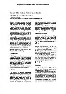
Figure 1: The computational grid at different times for Example 1 using the full (left two figures) and the local level set computations using the new coordinate system.

4.1

Example 1

This example is to test the local level set method using the proposed coordinates. The x-axis is the interface initially and we want to see how it changes under the velocity field generated by the following streamfunction [2] ψ=

1 sin2 [π(x + 0.5)] sin2 [π(y + 0.5)] . π

(10)

Figure 1 shows the solutions using the full version and the local version of the Lagrangian Computation at time t = 2.0. As mentioned before, in the case of large variations in the velocity field, the computational grid will be badly distorted, making the calculations not accuate (as shown in the first two figures in Figure 1). Using the same number of grids (60 by 60 in the full version and 10 by 360 in the local version), the local level set computations gives much better results. Similar to the Eulerian Computations, lots of information is wasted in the full Lagrangian Computations. Because we are only interested in the zero level set, memory saving local computations can be employed.

4.2

Example 2

We placed a circle of radius 0.15 centered at (0,0.25) at t = 0 and let it flows under the same velocity field as in Example 1. Figure 2 shows the solutions of the flow up to t = 2.0 using 100 by 100 grid points in the Eulerian Coordinates and the local level set computation using the Lagrangian Coordinates. It is clearly seen that Eulerian computations suffer from series numerical diffusion. The tail part was incorrectly removed in the Eulerian Coordinates. Because the velocity field is divergence-free, the flow is incompressible. To check the mass conservation of the region enclosed by the interface in different methods, we have checked the percentage change in the area. At the final time, t = 2.0, the Eulerian computations shows a 21.743% lost in mass, but a 0.342% gain in mass for the Lagrangian computations. With considering the approximation made in solving the ODE (9) and the approximation made in the Heaviside function when calculating the area, this little error is acceptable.

A Lagrangian Type Level Set Method Based on the Unified Coordinates

0.5

0.5

0.5

0.4

0.4

0.4

0.3

0.3

0.3

0.2

0.2

0.2

0.1

0.1

0.1

0

0

0

−0.1

−0.1

−0.1

−0.2

−0.2

−0.2

−0.3

−0.3

−0.3

−0.4

−0.4

−0.4

−0.5 −0.5

−0.5 −0.5

−0.4

−0.3

−0.2

−0.1

0

0.1

0.2

0.3

0.4

0.5

−0.4

−0.3

−0.2

−0.1

0

0.1

0.2

0.3

0.4

0.5

−0.5 −0.5

0.5

0.5

0.5

0.4

0.4

0.4

0.3

0.3

0.3

0.2

0.2

0.2

0.1

0.1

0.1

0

0

0

−0.1

−0.1

−0.1

−0.2

−0.2

−0.2

−0.3

−0.3

−0.3

−0.4

−0.4

−0.5 −0.5

−0.4

−0.3

−0.2

−0.1

0

0.1

0.2

0.3

0.4

0.5

−0.5 −0.5

−0.3

−0.2

−0.1

0

0.1

0.2

0.3

0.4

0.5

−0.5 −0.5

0.5

0.5

0.4

0.4

0.4

0.3

0.3

0.3

0.2

0.2

0.2

0.1

0.1

0.1

0

0

0

−0.1

−0.1

−0.1

−0.2

−0.2

−0.2

−0.3

−0.3

−0.3

−0.4

−0.4

−0.4

−0.3

−0.2

−0.1

0

0.1

0.2

0.3

0.4

0.5

−0.5 −0.5

−0.3

−0.2

−0.1

0

0.1

0.2

0.3

0.4

0.5

−0.5 −0.5

0.5

0.5

0.4

0.4

0.4

0.3

0.3

0.3

0.2

0.2

0.2

0.1

0.1

0.1

0

0

0

−0.1

−0.1

−0.1

−0.2

−0.2

−0.2

−0.3

−0.3

−0.3

−0.4

−0.4

−0.4

−0.3

−0.2

−0.1

0

0.1

0.2

0.3

0.4

0.5

−0.5 −0.5

−0.3

−0.2

−0.1

0

0.1

0.2

0.3

0.4

0.5

−0.5 −0.5

0.5

0.5

0.4

0.4

0.4

0.3

0.3

0.3

0.2

0.2

0.2

0.1

0.1

0.1

0

0

0

−0.1

−0.1

−0.1

−0.2

−0.2

−0.2

−0.3

−0.3

−0.3

−0.4

−0.4

−0.4

−0.3

−0.2

−0.1

0

0.1

0.2

0.3

0.4

0.5

−0.5 −0.5

−0.2

−0.1

0

0.1

0.2

0.3

0.4

0.5

−0.4

−0.3

−0.2

−0.1

0

0.1

0.2

0.3

0.4

0.5

−0.4

−0.3

−0.2

−0.1

0

0.1

0.2

0.3

0.4

0.5

−0.4

−0.3

−0.2

−0.1

0

0.1

0.2

0.3

0.4

0.5

−0.4

−0.3

−0.2

−0.1

0

0.1

0.2

0.3

0.4

0.5

−0.4

−0.4

0.5

−0.5 −0.5

−0.3

−0.4

−0.4

0.5

−0.5 −0.5

−0.4

−0.4

−0.4

0.5

−0.5 −0.5

6

−0.4

−0.4

−0.3

−0.2

−0.1

0

0.1

0.2

0.3

0.4

0.5

−0.5 −0.5

Figure 2: Interface at t = 0.4, 0.8, 1.2, 1.6 and 2.0 for Example 2 using the Eulerian Coordinates and the local Lagrangian Coordinates with the computational grids.

A Lagrangian Type Level Set Method Based on the Unified Coordinates

4.3

7

Example 3

For external driven flow like the one given in Example 1, the characteristics are linear and, therefore, should never intersect in the t − x − y space. This means that if there are two separated regions initially at t = t0 , the boundaries will never touch each other at later time t > t0 . Or, in other words, if the flow started with one connected component, it should never break. The merging and breaking of the interface corresponds to the intersection and separation of characteristics and these should not happen in this linear case. Following Example 2, three more circles are placed at (-0.25,0), (0.25,0) and (0,-0.25) under the same velocity field. The purpose of this example is to show that the Eulerian Coordinates computations produce a wrong solution when the two interfaces are moving too close together. Figure 3 shows the solution using only 60 by 60 grid points at time from 0.2 to 1.0. Because the interfaces are moving too close together, Eulerian computations (the first column) incorrectly merged them together at some time around t = 0.6. Although we have only 60 grid cells in one direction, the resolution of the Lagrangian level set method gives reasonably good result, as shown in the second and third columns in Figure 2. The interfaces do not merge together, due to the local refinement of the computational cells near the gap and the fact that the dissipation is minimized.

4.4

Example 4

The next example is the classic example called the Zalesak test. A rigid body is rotated in a zero vorticity field given by f = −y and g = x. The width of the slot is 0.02 and the length is 0.25. Here, we only use 16 by 16 grids in both x and y direction, with initial domain [−0.2, 0.2].2 in the real space. Figure 4 shows the solution of the Eulerian Coordinates at different times t = iπ/3 where i equals 1 to 6. This test is difficult for Eulerian computation, due to the fact that the width of the slot here is only resolved by 1 grid cell, as shown in Figure 5. Small numerical dissipation can destroy the shape completely. As shown in Figure 4(a), the slot disappears after t = 2π/3. Figure 4(b) shows the superior of the Lagrangian level set method. The shape is exactly the same as the initial one by using only 15 by 15 grid points in computation. The computation is very fast and efficient. Because the vorticity of the flow is zero, as shown in Figure 5, there is no distortion in the grid at all.

4.5

Example 5

All examples above can, of course, be solved by other type of Lagrangian-based methods relatively easily. However, as discussed above, in the case of the motion in the normal velocity, addition or deletion of characteristics make those methods difficult to implement. In this example, and the next, we will see that the proposed coordinates can handle topological change naturally. In this example, we again use the same external driven flow field as in Example 1, but add a normal velocity term with vn = 0.25. Four circles with radius 0.1 centered at (0.2,0), (-0.2,0), (0,0.2) and (0,-0.2) are used in the initial condition. Different from Example 3, the bodies in this case will merge together, due to the normal direction motion. Figure 6 shows the solutions using the proposed coordinates system at time between 0.1 to 0.5. Topological change in the solutions is simple to handle, as in the original level set method.

A Lagrangian Type Level Set Method Based on the Unified Coordinates

0.5

0.5

0.5

0.4

0.4

0.4

0.3

0.3

0.3

0.2

0.2

0.2

0.1

0.1

0.1

0

0

0

−0.1

−0.1

−0.1

−0.2

−0.2

−0.2

−0.3

−0.3

−0.3

−0.4

−0.4

−0.4

−0.5 −0.5

−0.5 −0.5

−0.4

−0.3

−0.2

−0.1

0

0.1

0.2

0.3

0.4

0.5

−0.4

−0.3

−0.2

−0.1

0

0.1

0.2

0.3

0.4

0.5

−0.5 −0.5

0.5

0.5

0.5

0.4

0.4

0.4

0.3

0.3

0.3

0.2

0.2

0.2

0.1

0.1

0.1

0

0

0

−0.1

−0.1

−0.1

−0.2

−0.2

−0.2

−0.3

−0.3

−0.3

−0.4

−0.4

−0.5 −0.5

−0.4

−0.3

−0.2

−0.1

0

0.1

0.2

0.3

0.4

0.5

−0.5 −0.5

−0.3

−0.2

−0.1

0

0.1

0.2

0.3

0.4

0.5

−0.5 −0.5

0.5

0.5

0.4

0.4

0.4

0.3

0.3

0.3

0.2

0.2

0.2

0.1

0.1

0.1

0

0

0

−0.1

−0.1

−0.1

−0.2

−0.2

−0.2

−0.3

−0.3

−0.3

−0.4

−0.4

−0.4

−0.3

−0.2

−0.1

0

0.1

0.2

0.3

0.4

0.5

−0.5 −0.5

−0.3

−0.2

−0.1

0

0.1

0.2

0.3

0.4

0.5

−0.5 −0.5

0.5

0.5

0.4

0.4

0.4

0.3

0.3

0.3

0.2

0.2

0.2

0.1

0.1

0.1

0

0

0

−0.1

−0.1

−0.1

−0.2

−0.2

−0.2

−0.3

−0.3

−0.3

−0.4

−0.4

−0.4

−0.3

−0.2

−0.1

0

0.1

0.2

0.3

0.4

0.5

−0.5 −0.5

−0.3

−0.2

−0.1

0

0.1

0.2

0.3

0.4

0.5

−0.5 −0.5

0.5

0.5

0.4

0.4

0.4

0.3

0.3

0.3

0.2

0.2

0.2

0.1

0.1

0.1

0

0

0

−0.1

−0.1

−0.1

−0.2

−0.2

−0.2

−0.3

−0.3

−0.3

−0.4

−0.4

−0.4

−0.3

−0.2

−0.1

0

0.1

0.2

0.3

0.4

0.5

−0.5 −0.5

−0.2

−0.1

0

0.1

0.2

0.3

0.4

0.5

−0.4

−0.3

−0.2

−0.1

0

0.1

0.2

0.3

0.4

0.5

−0.4

−0.3

−0.2

−0.1

0

0.1

0.2

0.3

0.4

0.5

−0.4

−0.3

−0.2

−0.1

0

0.1

0.2

0.3

0.4

0.5

−0.4

−0.3

−0.2

−0.1

0

0.1

0.2

0.3

0.4

0.5

−0.4

−0.4

0.5

−0.5 −0.5

−0.3

−0.4

−0.4

0.5

−0.5 −0.5

−0.4

−0.4

−0.4

0.5

−0.5 −0.5

8

−0.4

−0.4

−0.3

−0.2

−0.1

0

0.1

0.2

0.3

0.4

0.5

−0.5 −0.5

Figure 3: Interface at t = 0.2, 0.4, 0.6, 0.8 and 1.0 for Example 3 using the Eulerian Coordinates and the Lagragian Coordinates.

A Lagrangian Type Level Set Method Based on the Unified Coordinates

(a)

0.5

0.5

0.4

0.4

0.3

0.3

0.2

0.2

0.1

0.1

0

0

−0.1

−0.1

−0.2

−0.2

−0.3

−0.3

−0.4

−0.4

−0.5 −0.5

−0.4

−0.3

−0.2

−0.1

0

0.1

0.2

0.3

0.4

0.5

(b)

−0.5 −0.5

−0.4

−0.3

−0.2

−0.1

9

0

0.1

0.2

0.3

0.4

0.5

Figure 4: Interface at t = 2π for Example 4 using (a) the Eulerian Coordinates (h = 0) and (b) the local computations using the Lagrangian Coordinates.

0.5

0.5

0.5

0.4

0.4

0.4

0.3

0.3

0.3

0.2

0.2

0.2

0.1

0.1

0.1

0

0

0

−0.1

−0.1

−0.1

−0.2

−0.2

−0.2

−0.3

−0.3

−0.3

−0.4

−0.4

−0.5 −0.5

−0.4

−0.3

−0.2

−0.1

0

0.1

0.2

0.3

0.4

0.5

−0.4

−0.5 −0.5

−0.4

−0.3

−0.2

−0.1

0

0.1

0.5

0.5

0.4

0.4

0.3

0.3

0.2

0.2

0.1

0.1

0

0

−0.1

−0.1

−0.2

−0.2

−0.3

−0.3

−0.4

−0.5 −0.5

0.2

0.3

0.4

0.5

−0.5 −0.5

−0.4

−0.3

−0.2

−0.1

0

0.1

0.2

0.3

0.4

0.5

−0.4

−0.4

−0.3

−0.2

−0.1

0

0.1

0.2

0.3

0.4

0.5

−0.5 −0.5

−0.4

−0.3

−0.2

−0.1

0

0.1

0.2

0.3

0.4

0.5

Figure 5: The computational grid at different times for Example 4 using the local level set computations using the Lagrangian Coordinates.

A Lagrangian Type Level Set Method Based on the Unified Coordinates

0.5

0.5

0.4

0.4

0.3

0.3

0.2

0.2

0.1

0.1

0

0

−0.1

−0.1

−0.2

−0.2

−0.3

−0.3

−0.4

−0.4

−0.5 −0.5

−0.4

−0.3

−0.2

−0.1

0

0.1

0.2

0.3

0.4

0.5

−0.5 −0.5

0.5

0.5

0.4

0.4

0.3

0.3

0.2

0.2

0.1

0.1

0

0

−0.1

−0.1

−0.2

−0.2

−0.3

−0.3

−0.4

−0.4

−0.5 −0.5

−0.4

−0.3

−0.2

−0.1

0

0.1

0.2

0.3

0.4

0.5

−0.5 −0.5

10

−0.4

−0.3

−0.2

−0.1

0

0.1

0.2

0.3

0.4

0.5

−0.4

−0.3

−0.2

−0.1

0

0.1

0.2

0.3

0.4

0.5

Figure 6: Interface at t = 0.1 to 0.5 for Example 5 using the proposed coordinates with grids.

A Lagrangian Type Level Set Method Based on the Unified Coordinates 0.5

0.5

0.5

0.4

0.4

0.4

0.3

0.3

0.3

0.2

0.2

0.2

0.1

0.1

0.1

0

0

0

−0.1

−0.1

−0.1

−0.2

−0.2

−0.2

−0.3

−0.3

−0.3

−0.4

−0.4

−0.4

−0.5 −0.5

−0.4

−0.3

−0.2

−0.1

0

0.1

0.2

0.3

0.4

0.5

−0.5 −0.5

−0.4

−0.3

−0.2

−0.1

0

0.1

0.2

0.3

0.4

0.5

−0.5 −0.5

0.5

0.5

0.5

0.4

0.4

0.4

0.3

0.3

0.3

0.2

0.2

0.2

0.1

0.1

0.1

0

0

0

−0.1

−0.1

−0.1

−0.2

−0.2

−0.2

−0.3

−0.3

−0.3

−0.4

−0.4

−0.4

−0.5 −0.5

−0.5 −0.5

−0.4

−0.3

−0.2

−0.1

0

0.1

0.2

0.3

0.4

0.5

−0.4

−0.3

−0.2

−0.1

0

0.1

0.2

0.3

0.4

0.5

−0.5 −0.5

11

−0.4

−0.3

−0.2

−0.1

0

0.1

0.2

0.3

0.4

0.5

−0.4

−0.3

−0.2

−0.1

0

0.1

0.2

0.3

0.4

0.5

Figure 7: First row: Interface at t=1.0 for Example 6 using the Eulerian Coordinates with 60-by-60, 90-by-90 and 120-by-120 grids. Second row: the Lagrangian Coordinates using 60-by-60 grids at t=1.0. Computational grids at t=0.8 and 1.0.

4.6

Example 6

With the same external velocity field, we change the sign of the normal velocity, making the surface collapsed. The radius of the circles is now changed to 0.2 initially. The centers of the circles are now at (0.25,0), (-0.25,0), (0,0.25) and (0,-0.25) respectively. This example shows that the resolution of a Lagrangian computations is comparable to that of the Eulerian computations with 4 times number of grids.

5

Conclusion

We proposed a new Lagrangian-type Level Set Method which can eliminate the numerical dissipation completely in the Eulerian based Level Set Method. Topological change from the nonlinear motion can be handled naturally. No explicit treatment in the intersection of the characteristics is needed.

6

Acknowledgment

The author thanks D. Enright, S. Osher and J.L. Qian for some valuable suggestions.

A Lagrangian Type Level Set Method Based on the Unified Coordinates

7

12

Appendix: Level Set Dictionary in the Proposed Coordinates

In the appendix, we will translate some useful expressions and equations used in Eulerian based level set method to those corresponding in the new coordinates. All the following expressions can be calculated directly using the coordinate transformation given in section (??).

7.1

Gradient µ

∇φ =

7.2

N ∂φ M ∂φ −B ∂φ A ∂φ − , + ∆ ∂ξ ∆ ∂η ∆ ∂ξ ∆ ∂η

¶

(11)

Normal vector ³

∂φ ∂φ ∂φ N ∂φ ∂ξ − M ∂η , −B ∂ξ + A ∂η

´

~ = ∇φ = r N ³ ´2 ³ ´2 |∇φ| ∂φ ∂φ a ∂φ + 2b ∂φ ∂ξ ∂ξ ∂η + c ∂η

(12)

where a = B 2 + N 2 , b = −(AB + M N ) and c = A2 + M 2 .

7.3

Higher derivatives

To calculate curvature, κ, of the interface, we need to approximate the second derivative of the level set function φ in the spacial variables x and y. In the transformed coordinates, they becomes ∂2φ ∂x2

=

1 ∆2

Ã

2 ∂2φ 2∂ φ N + M − 2M N ∂ξ 2 ∂ξ∂η ∂η 2

"

∂ + ∂η ∂2φ ∂y 2

=

1 ∆2

2∂

Ã

Ã

"

2φ

M2 ∆2

!

N ∂ − ∆ ∂ξ

µ

M ∆

¶#

∂ + ∂η

Ã

2φ

A2 ∆2

!

B ∂ − ∆ ∂ξ

µ

A ∆

¶#

"

∂ + ∂ξ

Ã

N2 ∆2

!

M ∂ − ∆ ∂η

µ

N ∆

¶#

∂φ ∂ξ

∂φ , ∂η

2 ∂2φ 2∂ φ B + A − 2AB ∂ξ 2 ∂ξ∂η ∂η 2 2∂

!

(13) !

"

∂ + ∂ξ

Ã

B2 ∆2

!

A ∂ − ∆ ∂η

µ

B ∆

¶#

∂φ ∂ξ

∂φ ∂η

(14)

and ∂2φ ∂x∂y

"

#

1 ∂2φ ∂2φ ∂2φ = −BN + (AN + BM ) − AM ∆2 ∂ξ 2 ∂ξ∂η ∂η 2 · µ ¶ µ ¶¸ · µ ¶ µ ¶¸ 1 ∂ B ∂ B ∂φ 1 ∂ A ∂ A ∂φ + −N +M + N −M ∆ ∂ξ ∆ ∂η ∆ ∂ξ ∆ ∂ξ ∆ ∂η ∆ ∂η

(15)

A Lagrangian Type Level Set Method Based on the Unified Coordinates

7.4

13

Volume integral Z

Z Ω

f (x, y)H(−φ(x, y))dxdy =

Ω

f (ξ, η)H(−φ(ξ, η))∆dξdη ,

(16)

where H(φ) is the smoothed Heaviside function given by 1 H(φ) = [1 + f (φ) + (f (φ) − 1)sign(² − φ)][1 + sign(² + φ)] 4 with

µ

f (φ) =

1 φ 1 πφ + + sin 2 2² 2π ²

(17)

¶

(18)

and ² is normally taken to be 1.5 min(dξ, dη).

7.5

Reinitialization equation

In the original setting of level set method, reinitialization plays a very important role. To reduce the error in determining the zero level set from interpolation, it is desirable to keep the level set function a signed distance function. This is even important when the zero level set tends to fold making the interface close to each other. However, as mentioned earlier in section (??), we don’t need to do the reinitialization, due to the fact that the grid will re-adjust itself so that the narrow region will be resolved by more grid points. We here give the formulation of the reinitialization equation in the proposed coordinates, but emphasis that we do not need to apply it to our level set function at all. s µ

∂φ sign(φ0 )  ∂φ + a ∂τ ∆ ∂ξ

¶2

µ

∂φ ∂φ ∂φ +c + 2b ∂ξ ∂η ∂η

¶2



− ∆ = 0 ,

(19)

with a, b and c defined above in section (??).

7.6

Orthogonalization equation

The equation orthogonally extending some quantity, ψ, from the interface in the x − y space will be given by h

³

´

³

∂φ ∂φ ∂φ ∂φ ∂ψ sign(φ) N N ∂ξ − M ∂η + B B ∂ξ − A ∂η r ³ ´ + ³ ´2 2 ∂τ ∂φ ∂φ ∂φ ∆ a ∂φ + 2b + c ∂ξ ∂ξ ∂η ∂η

h

+

³

´

³

∂φ ∂φ ∂φ sign(φ) −M N ∂φ ∂ξ − M ∂η + A B ∂ξ − A ∂η

r ³

∆ a

∂φ ∂ξ

´2

∂φ + 2b ∂φ ∂ξ ∂η + c

³

∂φ ∂η

´2

´i

∂ψ ∂ξ ´i

∂ψ ∂η

= 0.

(20)

References [1] Y. Chang, T. Hou, B. Merriman & S. Osher, A Level Set Formulation of Eulerian Interface Capturing Methods for Incompressible Fluid Flows, J. Comput. Phys., 124, 449-464, (1996).

A Lagrangian Type Level Set Method Based on the Unified Coordinates

14

[2] D. Enright, R. Fedkiw, J. Ferziger & I. Mitchell, A Hybrid Particle Level Set Method for Improved Interface Capturing, J. Comput. Phys., 183, 83-116, (2002). [3] W.H. Hui, P.Y. Li & Z.W.Li, A Unified Coordinate System for Solving the Two-dimensional Euler Equations, Journal of Computational Physics, 153, 596-673. [4] W.H. Hui & S. Koudriakov, Computation of the Shallow Water Equations Using the Unified Coordinates, SIAM J. Sci. Comput., 23, 1615-1654 (2002). [5] W.H. Hui & S. Koudriakov, A Unified Coordinate System for Solving the Three-dimensional Euler Equations, J. Comput. Phys. 172, 235-260, (2001). [6] G.S. Jiang & D. Peng, Weighted ENO Schemes for Hamilton Jacobi Equations, SIAM J. Sci. Comput., 21(6), 2126, 2000. [7] R.J. Leveque, Finite Volume Methods for Hyperbolic Problems, Cambridge, 2002. [8] W. Mulder, S. Osher & J. Sethian, Computing Interface Motion in Compressible Gas Dynamics, J. Comput. Phys., 100, 209-228, (1992). [9] S. Osher & R. Fedkiw, Level Set Methods and Dynamic Implicit Surfaces, Springer, 2003. [10] S. Osher & J.A. Sethian, Fronts Propagating with Curvature-dependent Speed: Algorithm Based on Hamilton-Jacobi Formulations, J. Comput. Phys., 79, 12-49, (1988). [11] J.L. Qian & S.Y. Leung, A Level Set Based Eulerian Method for Paraxial Multivalued Traveltimes, in preparations. [12] W. Rider & D. Kothe, Stretching and Tearing Interface Tracing Methods, 12th AIAA CFD Conference, 95-1717, AIAA, 1995. Can be found here http://public.lanl.gov/mww/publicas.html [13] C.W. Shu & S. Osher, Efficient Implementation of Essentially Nonoscillatory Shockcapturing Schemes, Journal Of Computational Physics, 77, 439, 1988. [14] M. Sussman, P. Smereka & S. Osher, A Level Set Approach for Computing Solutions to Incompressible Two-phase Flows, J. Comput. Phys., 114, 146-159, (1994). [15] D.J. Torres & J.U. Brackbill, The Point-Set Method: Front-Tracking Without Connectivity, J. Comput. Phys., 165, 620-644, (2000). [16] G. Tryggvason, B. Bunner, A. Esmaeeli, D. Juric, N. Al-Rawahi, W. Tauber, J. Han, S. Nas & Y.J. Jan, A Front-Tracking Method for the Computations of Multiphase Flow, J. Comput. Phys., 169, 708-759, (2001).