Page 2 .... Substitute dx and dy in Eq. 1 and rearrange dg = gx(vxds + uxdt) + gyuydt+. +(gxx + gyy)uzdt + gsds + gtdt = 0. (6). This is a BCCE for combined scene ...
IEEE Workshop on Motion and Video Computing, 2002, Orlando, Florida, USA
A Linear Model for Simultaneous Estimation of 3D Motion and Depth 1
Hanno Scharr1,2,3 and Ralf K¨ usters1,2 Institute for Chemistry and Dynamics of the Geosphere, Institute III: Phytosphere Forschungszentrum J¨ ulich GmbH, 52425 J¨ ulich, Germany 2 Interdisciplinary Center for Scientific Computing, Ruprecht Karls University, Im Neuenheimer Feld 368, 69120 Heidelberg, Germany 3 Intel Research, 2200 Mission College Blvd, Santa Clara, CA 95054, USA {Hanno.Scharr,Ralf.Kuesters}@iwr.uni-heidelberg.de
ABSTRACT A novel model for simultaneous estimation of full 3D motion and 3D position in world coordinates from multi camera sequences is presented. To this end scene flow [29] and disparity are estimated in a single estimation step. The key idea is to interpret sequences of 2 or more cameras as one 4D data set. In this 4D space a given motion model, a camera model and a brightness change model are combined into a brightness change constraint equation (BCCE) combining changes due to object motion and different camera positions. The estimation of parameters in this constraint equation is demonstrated using a weighted total least squares estimator called structure tensor. An evaluation of systematic errors and noise stability for a 5 camera setup is shown as well as results on synthetic sequences with ground truth and data acquired under controlled laboratory conditions.
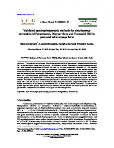
as well (e.g. the ones in [1, 14]). In state of the art optical flow algorithms for motion estimation an image sequence of a single fixed camera is interpreted as data in a 3D x-y-t-space. In this space a BCCE defines a linear model for the changes of gray values due to local object motion and other parameters of e.g. illumination changes or physical processes (compare e.g. [13]). The result of the calculation then is a displacement vector field, i.e. local object motion and quantities of brightness change if an appropriate model is used. Using a moving camera looking at a fixed scene identical algorithms can be used to determine object depth, known as structure from camera motion (e.g. [20]). The basic idea for the new estimation technique presented here is to interpret the camera position s as a new dimension (see Fig. 1). Hence all image sequences acquired by a multi camera setup (or a pseudo multi camera setup as in our target application mentioned below) are combined to sample a 4D-Volume in x-y-st-space. If a 2D camera grid is used (as e.g. in [22] ) we get a 5D-Volume in x-y-sx-sy -t-space. This paper is restricted to the 4D case. In [5] a 2D-manifold is constructed combining all 1D trajectories of a surface point acquired by multiple cameras. This comes very close to the idea presented here. The advantage of our approach is that it is an extension of usual optical flow and consequently can easily be combined with other methods and extensions stated in the related work section. In our target application plant growth shall be studied using a single camera on a linear moving stage. For convenience, let the camera translate along its x-axis and denote its position by s (see Fig. 1). From other plant growth studies (e.g. [24]) we know that plant
KEY WORDS optical flow, scene flow, multiple cameras, disparity, depth, 3D motion
1
Introduction
Motion estimation as well as disparity estimation are standard tasks for optical flow algorithms as well known from early publications (e.g. [16, 21] and many more). This paper aims to combine both scene flow [29] (i.e. 3D optical flow estimated from 2D sequences) and disparity estimation within a single optical-flowlike estimation step. As the developed model has the same form as usual brightness change constraint equations (BCCE) no special estimation framework has to be established. We use the so called structure tensor method [3, 15, 17] but other methods can be applied 1
a
b
Z
quired by N cameras that differ only in their Xs positions (see Fig. 1), where s denotes the camera index s ∈ {−N/2, N/2}. The camera positions are equidistant with distance VX and thus the camera positions are Xs = VX s. We define an s-axis parallel to the world coordinate axis X. The gray values g acquired by such a multi camera setup can be stored in a 4D x-y-s-t-space, where x and y denote the pixel grid coordinates, camera position s and time t. We start the derivation of the new BCCE with the total differential of the gray values g(x, y, s, t), combined with the brightness change model dg/dt = 0 ↔ dg = 0
P
P
Z
y Z Z
Y
x
f
image plane
p
Xs
X
p
Y
x
X and s
y f
Xs
image plane x
x
X
X and s
Figure 1. Projection of a point P by a pinhole camera a in 2D and b in 3D.
dg(x, y, s, t) = gx dx + gy dy + gs ds + gt dt = 0
We use the notation g∗ = ∂g ∂∗ for spatio-temporal derivatives of the gray values g. As motion model for a point in world coordinates (X, Y, Z) we choose
motion can be measured by optical flow using a frame rate of less than one image per minute. Thus if image sequence acquisition with the moving stage is done within a few seconds our scene can be interpreted to be fixed for this time interval. Then the acquired image sequence samples a volume in x-y-s-space at a fixed point in time. In the remainder of this paper we treat our single camera on moving stage setup as a (pseudo) multi camera setup acquiring at a single point in time.
(X, Y, Z)(t) = (X0 , Y0 , Z0 ) + (UX , UY , UZ ) t
(2)
with the center point (X0 , Y0 , Z0 ) of a surface element and its velocity (UX , UY , UZ ). Projecting it by a pinhole camera at position Xs = VX s (see Fig. 1) the image coordinates x and y are x = f (X − VX s)/Z and y = f Y /Z and thus we get � � � � f x X0 − VX s + UX t (s, t) = (3) y Y0 + UY t Z0 + UZ t
Related work. There is rich literature on optical flow estimation techniques (see [1, 14] for current overviews) and many extensions have been developed. There are extensions towards affine motion estimation [8, 9], scene flow [29] and physically motivated brightness changes [6, 12, 13]. Robust estimations [4, 11], variational approaches [16, 31, 32], coarseto-fine schemes [2], regularization schemes [19, 26], special filters [10, 7, 18] and coupled denoising methods [27] have been studied. There already exist frameworks for simultaneous motion and stereo analysis (e.g. [28, 30, 5]). But to the best of our knowledge no BCCElike linear model for simultaneous estimation of disparity and optical flow has been presented so far. Paper organization. We start by the derivation of the new model in 4D (Sec. 2) followed by a compact revision of the structure tensor (Sec. 3). An experimental validation of the novel model within this estimation framework is presented in Sec. 4. Finally we conclude with a summary in Sec. 5.
2
(1)
and the differentials dx = dy =
f x Z0 +UZ t ((UX − UZ f )dt f y Z0 +UZ t (UY − UZ f )dt
− VX ds)
Using the approximation |Z0 | � |UZ t| UZ t ≈ Z0 and substituting
⇔
disparity vx := −f VX /Z0 optical flow ux := f UX /Z0 , uy := f UY /Z0 divergence uz := −UZ /Z0
(4) Z0 +
(5)
the differentials dx and dy become dx = ux dt + uz xdt + vx ds
dy = uy dt + uz ydt
Substitute dx and dy in Eq. 1 and rearrange dg
= gx (vx ds + ux dt) + gy uy dt+ +(gx x + gy y)uz dt + gs ds + gt dt = 0
(6)
This is a BCCE for combined scene flow and disparity estimation. Expression (gx x + gy y)uz is well known from affine motion models (e.g.[8, 9]). There it is used for divergence estimation when x and y are local not global image coordinates. Using the structure tensor framework (compare Sec. 3) the expression
Derivation of the new BCCE
In this section the novel BCCE shall be developed, given a motion model, a camera model and a brightness change model. Image sequences are ac2
Using a matrix D composed of the vectors d�i via Dij = (d�i )j Eq. 11 becomes D� p = �e. We minimize �e using a weighted 2-norm
(gx x + gy y)uz dt leads to instable estimates. We circumvent this problem by introducing local coordinates (�x, �y) = x0 + (x − x0 ) = y0 + (y − y0 )
x y
=: x0 + �x =: y0 + �y
!
p =: p�T J� p = min ||�e|| = ||D� p|| = �pT DT WD�
(7)
where W is a diagonal matrix containing the weights. In our case Gaussian weights are used (see Sec. 4). It multiplies each equation i in Eq. 11 by a weight wi . The matrix J = DT WD is the so called structure tensor. The error �e is minimized by introducing the assumption |p�˜| = 1 in order to suppress the trivial solution �p˜ = �0. Doing so the space of solutions p�˜ is spanned by the eigenvector(s) to the smallest eigenvalue(s) of J. We call this space the null space of J as the smallest eigenvalue(s) are 0 if the model is ideally fulfilled, i.e. �e = �0. Usually the model is not ideally fulfilled and the eigenvectors to eigenvalues below a given threshold are used to span this space. In the case of standard optical flow the null space of J is 1D as only data variations with respect to time are regarded [13]. In our case variations with respect to camera position and time are considered. Thus using the novel BCCE the null space of J is a 2D manifold. It is spanned by the eigenvectors p�˜1 and p�˜2 of the smallest two eigenvalues of J. Disparity vx is calculated from these eigenvectors via a linear combination �p˜s = α1 �p˜1 + α2 p�˜2 with a vanishing fifth entry (i.e. dt = 0 in Eq. 10). Thus p�˜s = (vx ds, 0, 0, ds, 0)T . Disparity vx then is vx = p˜s1 /˜ ps4 . Scene flow �u is calculated via a linear combination p�˜t = β1 �p˜1 + β2 �p˜2 with a vanishing fourth entry (i.e. ds = 0 in Eq. 10). Thus p�˜t = ((ux + x0 uz )dt, (uy + y0 uz )dt, uz dt, 0, dt)T . We first calculate uz via uz = pt5 and then get ux = p˜t1 /˜ pt4 − x0 uz and uy = p˜t3 /˜ p˜t2 /˜ pt4 − y0 uz for each pixel (x0 , y0 ). Knowing �u and vx we recover 3D motion and depth in world coordinates using Eq. 5.
for each local neighborhood used by the structure tensor, where (x0 , y0 ) denotes the center pixel of the local neighborhood. Eq. 6 then becomes = gx (vx ds + (ux + x0 uz )dt)+ +gy (uy + y0 uz )dt+ +(gx �x + gy �y)uz dt+ +gs ds + gt dt = 0
dg
(8)
In the next section we revisit the structure tensor estimator and demonstrate how to determine the parameters in Eq. 8.
3
Revision of the Structure Tensor
In this total least squares parameter estimation method a model with linear parameters pi has to be given in the form d�T p� = 0 (9) with data vector d� and parameter vector � p. Rewriting our BCCE (Eq. 8) using d� = p� =
(gx , gy , gx �x + gy �y, gs , gt )T (vx ds + (ux + x0 uz )dt, (uy + y0 uz )dt, uz dt, ds, dt)T
(10)
we recover this form. Eq. 9 is one equation for several parameters (the components of the parameter vector) and thus under determined. In our case we have one equation for each 4D pixel. Thus we can add the assumption, that within a small 4D neighborhood Ω of pixels i all equations are approximately solved by the same set of parameters � p. Eq. 9 therefore becomes � = ei for all pixels i in Ω d�T i p
(12)
4
Experimental Validation
(11) This section illustrates the successful application of the introduced scheme. In all experiments described here, we use optimized separable derivative kernels [23]. They are composed of a 1D derivative kernel D = [0.0838, 0.3324, 0, −0.3324, −0.0838] and smoothing kernels S in all other directions where S = [0.0234, 0.2416, 0.4700, 0.2416, 0.0234]. From systematic test calculations [23] we know that cross talk between different components of the parameter vector p� (Eq. 9) is negligible for this filter choice. This allows us to only investigate accuracy of single parameters when all other parameters are constant, e.g. zero.
with errors ei which have to be minimized by the sought �˜. for solution p Suppose there is enough variation in the data. Then the data vectors d�i span the hole space. For usual optical flow estimation this is called the full flow case where all parameters can be estimated. If there is not enough structure in the data the so called aperture problem occurs. Then not all parameters can be estimated. This is called normal flow case. We only refer to the full flow case here as the handling of other cases can be deduced from literature (e.g. [25]). 3
a
b σn = λ = 4 pixel λ = 8 pixel λ = 16 pixel λ = 32 pixel
σ n = 0.025
0 rel. error of UX
rel. error of UX
The local neighborhood Ω (Eq. 11) and weights W (Eq. 12) were implemented by Gaussian filters B with standard deviations σ = 6 in x- and y-direction, σ = 0 in s- and σ = 1 in t-direction. These filters B have 25 pixel length for x- and y-direction, 5 pixel length for t-direction and no filter is applied in s-direction. The larger the standard deviations are the higher the noise stability and the smoother the results. For synthetic data with g ∈ {−1, 1} an eigenvalue of the structure tensor below τ = 0.0012 was considered to be zero.
velocity UX
c
velocity UX
d
In order to quantify the accuracy of the used algorithm we measure velocity and disparity of a translating fronto-parallel pattern
λ = 4 pixel λ = 8 pixel λ = 16 pixel λ = 32 pixel
velocity UZ
e
σn = 0.025
λ = 4 pixel λ = 8 pixel λ = 16 pixel λ = 32 pixel
velocity UZ
f
(13)
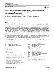
with wave numbers KX and KY in world coordinates. Compare Sec. 2 for further notation. In our tests we choose f = 10, Z(t0 ) = 100 at the estimation point of time t0 , VX = 1 and UX = 0, UY = 0, UZ = 0 when not varied (all in arbitrary units). Wave numbers kx and ky in image coordinates are kx = KX Z0 + UZ t/f and ky = KY Z0 + UZ t/f . They are chosen to be kx = ky = 2π/λ with λ ∈ {4, 8, 16, 32} pixel at t0 . We calculated � and depth Z for an imaginary set of the 3D velocity U five cameras. To those sequences no noise or Gaussian noise with a standard deviation σn = 0.025 (i.e. 2.5%) is added. Fig. 2a shows the relative error of the calculated X-velocity UX for different wavelengths without noise. This illustrates the systematic error due to numerical and filter inaccuracies. For UY results are identical. The run of the curves agrees well with comparable calculations for conventional optical flow [23]. The error stays below 0.03% for displacements UX below 4. Then smallest wavelengths produce severe errors as we come close to (inestimable) displacements near 0.5 λ. If we eliminate these wavelengths by smoothing larger displacements can be estimated accurately. Fig. 2c shows the relative error of the calculated Z-velocity UZ for no noise added. Thus the systematic error stays below 0.3% for UZ < 0.1 and below 3% for UZ < 1. Fig. 2e shows the relative error of the calculated depth Z for varying baseline widths VX . As calculations are similar to those for UX and UY error curves are very similar, too. Figs. 2b,d,f show the relative errors for 2.5% noise. This is realistic for CCD cameras used in our experiments. The relative errors rise severely for small values
λ = 4 pixel λ = 8 pixel λ = 16 pixel λ = 32 pixel
camera distance VX
σ n = 0.025 rel. error of Z
σn = 0
rel. error of Z
g(x, y, s, t) = cos(KX X) ∗ cos(KY Y ) Zt − UX t + VX s X = x Z0 +U f Z0 +UZ t − UY t Y =y f
rel. error of UZ
rel. error of UZ
σn = 0
4.1 Synthetic Data with Ground Truth
λ = 4 pixel λ = 8 pixel λ = 16 pixel λ = 32 pixel
λ = 4 pixel λ = 8 pixel λ = 16 pixel λ = 32 pixel
camera distance VX
Figure 2. Relative errors of the estimated velocity components UX , UZ and depth Z, calculated from synthetic data (Eq. 13) for different noises and wavelengths. Depth error is plotted for varying camera distances VX .
of UX , UZ or VX but stay between 0.1% and 1% for wide ranges of UX , UZ or VX . As we calculate UX and UY via optical flow components ux = p˜t1 /˜ pt4 − x0 uz and uy = p˜t2 /˜ pt4 − y0 uz there is an error propagation from UZ to UX and UY . In our target application usually UZ is very small thus the absolute error propagated to UX and UY is small, too.
4.2 Real Image Sequences To illustrate the correctness of the applied technique on real sequences, the results for a cube translating mainly in Z-direction viewed from five camera positions are presented. These sequences have been acquired under controlled laboratory conditions using a single camera on a moving stage as mentioned in the introduction. The cube’s edges have a length of 4.9 cm and it’s sides are figured with a noise pattern in order to have enough structure. The cube was set on a moving stage and repeatedly moved by a distance of about 4
5
a
b
c
d
UZ
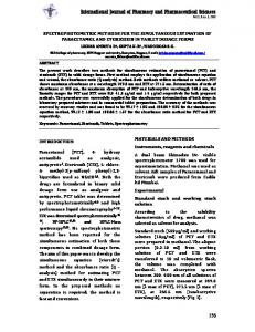
-1mm in Z-direction between consecutive images. The baseline of the camera positions was VX = 0.5 cm and the mean object-camera distance was ≈ 66 cm. Mean disparity was 38 pixel, thus we shifted the off center images by ±38 or ±76 pixel. By doing so we choose the depth working point of the algorithm, as derivative filters work best for displacements smaller than or around 1 pixel. Fig. 3a shows an original image of the sequence. Fig. 3b shows a top view of the cube rendered from the estimated depth chart. The front edge of the cube appears rounded off, apart from that the calculated surface is quite smooth due to the spatial smoothing in the structure tensor. The calculated position of the edge agrees well with the position in the original images. Please note that there is no additional smoothing or other regularization applied for visualization. In Fig. 3c the estimated Z-velocity UZ of the cube’s surface is greyvalue-coded, brighter areas correspond to higher velocities. Row 55 is marked, as Fig. 3d shows this row profile in order to illustrate the variation of UZ . In Fig. 3e estimated velocities multiplied by a factor 5 are drawn as arrows onto the cubes surface. Ideally they should be parallel and of identical length which is fulfilled quite well.
e
Summary and Conclusion
We have introduced a novel model for simultaneous estimation of scene flow and disparity in multi camera sequences. We demonstrated its use within the structure tensor estimation framework but due to its BCCElike form other optical flow methods as robust estimations, variational approaches, coarse-to-fine schemes or special regularizations may be applied as well. This will provide additional benefit e.g. more robust and/or faster performance. Using the structure tensor we have shown that this novel model results in accurate depth and 3D motion estimates in world coordinates with high density and noise stability. Systematic errors are low due to optimized filters. Tests using synthetic data with ground truth showed that estimation results are best when dominating image structures are above a wavelength λ = 4 pixel. Further in the presence of noise there are optimally estimable values of X-, Y velocity and disparity. Z-velocity should be at least one order of magnitude lower. For practical applications a depth working point has to be chosen by registering images globally with integer pixel accuracy. The presented method then performs the wanted differential subpixel estimation. We will consider this in the experimental design of our plant growth target application. As investigated plant surfaces, e.g. leafs, are
Figure 3. Results for the cube sequence: a estimated velocity ux greyvalue-coded with marked row, b row profile of the marked row, c disparity vx greyvalue-coded and d rendered height-field calculated from vx .
smooth we will further investigate regularizations or variational estimators and use more camera positions. More general camera positions will be investigated using our method together with appropriate rectification schemes as common in stereo applications. 5
This work has partly been funded by DFG (FOR240 Image sequence analysis to investigate dynamic processes and SPP1114 LOCOMOTOR).
[17] B. J¨ ahne. Spatio-temporal image processing, volume 751. Springer, Berlin, 1993. [18] B. J¨ ahne, H. Scharr, and S. K¨ orkel. Principles of filter design. In Handbook of Computer Vision and Applications. Academic Press, 1999. [19] T. Koivunen and A. Nieminen. Motion field restoration using vectormedian filtering on high definition television sequences. In Proc. Vis. Comm. and Im. Proc.’90, volume 1360, pages 736 – 742, 1990. [20] L.H.Matthies, R.Szeliski, and T.Kanade. Kalman filter-based algorithms for estimating depth from image sequences. IJCV, 3:209–236, 1989. [21] B. Lucas and T. Kanade. An iterative image registration technique with an application to stereo vision. In DARPA Im. Underst. Workshop, pages 121–130, 1981. [22] Y. Nakamura, T. Matsuura, K. Satoh, and Y. Ohta. Occlusion detectable stereo–occlusion patterns in camera matrix. In CVPR, pages 371–378, 1996. [23] H. Scharr. Optimal Operators in Digital Image Processing. PhD thesis, University of Heidelberg, Germany, 2000. [24] U. Schurr, A. Walter, S. Wilms, H. Spies, N. Kirchgessner, H. Scharr, and R. K¨ usters. Dynamics of leaf and root growth. In 12th Int. Con. on Photosynthesis, PS 2001, 2001. [25] H. Spies and B. J¨ ahne. A general framework for image sequence processing. In Fachtagung Informationstechnik, pages 125–132, Universit¨ at Magdeburg, 2001. [26] H. Spies, N. Kirchgeßner, H. Scharr, and B. J¨ ahne. Dense structure estimation via regularised optical flow. In VMV 2000, pages 57–64, Saarbr¨ ucken, Germany, 2000. [27] H. Spies and H. Scharr. Accurate optical flow in noisy image sequences. In ICCV’01, pages 587–592, Vancuver, Canada, 2001. [28] R. Szeliski. A multi-view approach to motion and stereo. In CVPR, 1999. [29] S. Vedula, S. Baker, P. Rander, R. Collins, and T. Kanade. Threedimensional scene flow. In ICCV 1999, pages 722–729, 1999. [30] S. Vedula, S. Baker, S. Seitz, R. Collins, and T. Kanade. Shape and motion carving in 6d. In CVPR 2000, pages 592–598, 2000. [31] J. Weickert. Applications of nonlinear diffusion in image processing and computer vision. Acta Math.Univ.Comenianae, Proc. of Algo. 2000, LXX(1):33 – 50, 2001. [32] J. Weickert and C. Schn¨ orr. Variational optic flow computation with a spatio-temporal smoothness constraint. Technical Report 15/2000, Comp. Vis., Graphics, and Patt. Recogn. Group, Dept. of Math. and Comp. Sci., Univ. Mannheim, Germany, July 2000.
References [1] J. Barron, D. Fleet, and S. Beauchemin. Performance of optical flow techniques. In IJCV, pages 43–77, 1994. 12(1). [2] J. Bergen, P. Burt, R. Hingorani, and S. Peleg. A three-frame algorithm for estimating two-component image motion. IEEE Transactions on Pattern Analysis and Machine Intelligence, 14(9):886–895, 1992. [3] J. Big¨ un and G. H. Granlund. Optimal orientation detection of linear symmetry. In ICCV, pages 433– 438, 1987. [4] M. Black, D. Fleet, and Y. Yacoob. Robustly estimating changes in image appearence. CVIU, 7(1):8–31, 2000. [5] R. Carceroni and K. Kutulakos. Multi-view 3d shape and motion recovery on the spatio-temporal curve manifold. In ICCV (1), pages 520–527, 1999. [6] T. S. J. Denney and J. L. Prince. Optimal brightness functions for optical flow estimation of deformable motion. IEEE Trans. Im. Proc., 3(2):178–191, 1994. [7] H. Farid and E. P. Simoncelli. Optimally rotationequivariant directional derivative kernels. In 7th Int’l Conf Computer Analysis of Images and Patterns, Kiel, 1997. [8] G. Farneb¨ ack. Fast and accurate motion est. using orient. tensors and param. motion models. In ICPR, pages 135–139, 2000. [9] D. Fleet. Measurement of Image Velocity. Kluwer, 1992. [10] D. Fleet and K. Langley. Recursive filters for optical flow. IEEE Transactions on Pattern Analysis and Machine Intelligence, 17(1), 1995. pp. 61-67. [11] C. Garbe. Measuring Heat Exchange Processes at the Air-Water Interface from Thermographic Image Sequence Analysis. PhD thesis, Heidelberg University, 2001. [12] S. Gupta and J. Prince. On variable brightness optical flow for tagged mri. In Information Processing in Medical Imaging, pages 323 – 334, 1995. [13] H. Haußecker and D. Fleet. Computing optical flow with physical models of brightness variation. PAMI, 23(6):661–673, June 2001. [14] H. Haußecker and H. Spies. Motion. In B. J¨ ahne, H. Haußecker, and P. Geißler, editors, Handbook of Computer Vision and Applications. Academic Press, 1999. [15] H. Haußecker, H. Spies, and B. J¨ ahne. Tensor-based image sequence processing techniques for the study of dynamical processes. In Proc. Int. Symp. On RealTime Imaging and Dynamic Analysis, volume 32(5), pages 704–711, Japan, 1998. [16] B. Horn and B. Schunk. Determining optical flow. In Art. Int., volume 17, pages 185–204, 1981.
6