Estimation of slope for linear regression model with uncertain prior information and Student-t error Shahjahan Khan Department of Mathematics and Computing Australian Centre for Sustainable Catchments University of Southern Queensland Toowoomba, Queensland, Australia Email:
[email protected] and A.K.Md.E. Saleh School of Mathematics and Statistics Carleton University, Ottawa, Canada Abstract This paper considers estimation of the slope parameter of the linear regression model with Student-t errors in the presence of uncertain prior information on the value of the unknown slope. Incorporating uncertain non-sample prior information with the sample data the unrestricted, restricted, preliminary test, and shrinkage estimators are defined. The performances of the estimators are compared based on the criteria of unbiasedness and mean squared errors. Both analytical and graphical methods are explored. Although none of the estimators is uniformly superior to the others, if the non-sample information is close to its true value, the shrinkage estimator over performs the rest of the estimators.
Keywords and Phrases: Multiple regression model; Student-t errors; preliminary test and shrinkage estimators; bias, mean square error and relative efficiency; mixture distribution of normal and inverted gamma; non-central chi-square and F distributions; and incomplete beta ratio. AMS 2000 Subject Classification: Primary 62F30, Secondary 62H12 and 62F10.
1
Introduction Customarily the classical estimators of unknown parameters are based exclusively on
the sample data. Such estimators disregard any other kind of non-sample prior information in its definition. The notion of inclusion of non-sample information to the estimation of parameters has been introduced to ‘improve’ the quality of the estimators. The natural expectation is that the inclusion of additional information would result in a better estimator. In some cases this may be true, but in many other cases the risk of worse 1
consequences can not be ruled out. A number of estimators have been introduced in the literature that, under particular situation, over performs the traditional exclusive sample data based unbiased estimators when judged by criteria such as the mean squared error and squared error loss function. In the wake of increasing criticism on the inappropriate use of the normal distribution to model the errors there is a growing trend to use, often more appropriate, Studentt model. Fisher (1956, p.133) warned against the consequences of inappropriate use of the traditional normal model. Fisher (1960, p.46) analyzed Darwin’s data (cf. Box and Taio, 1992, p. 133) by using a non-normal model. Fraser and Fick (1975) analyzed the same data by the Student-t model. Zellner (1976) provided both Bayesian and frequentist analyses of the multiple regression model with Student-t errors. Fraser (1979) illustrated the robustness of the Student-t model. Prucha and Kelegian (1984) proposed an estimating equation for the simultaneous equation model with the Student-t errors. Ullah and Walsh (1984) investigated the optimality of different types of tests used in econometric studies for the multivariate Student-t model. The interested readers may refer to the more recent work of Singh (1988), Lange et al. (1989), Giles (1991), Khan (1992), Anderson (1993), Spanos (1994), and Khan (1998) for different applications of the Student-t models. For a wide range of applications of the Student-t models refer to Lange et al. (1989). There has been many studies in the area of the ‘improved’ estimation following the seminal work of Bancroft (1944) and later Han and Bancroft (1968). They developed the preliminary test estimator that uses uncertain non-sample prior information (not in the form of prior distributions), in addition to the sample information. Stein (1956) introduced the Stein-rule (shrinkage) estimator for multivariate normal population that dominates the usual maximum likelihood estimators under the squared error loss function. In a series of papers Saleh and Sen (1978, 1985) explored the preliminary test approach to Stein-rule estimation. Many authors have contributed to this area, notably Sclove et al. (1972), Judge and Bock (1978), Stein (1981), Maatta and Casella (1990), and Khan (1998), to mention a few. Khan and Saleh (1995, 1997) investigated the problem for a family of Student-t populations. However, the relative performance of the preliminary test and shrinkage estimators of the slope parameter of linear regression model with Student-t error has not been investigated. It is well known that the mle of the slope parameter is unbiased. We wish to search for an alternative estimator of the slope parameter that is biased but may well have some superior statistical property in terms of another more popular statistical criterion, namely the mean square error. In this process, we define three biased estimators: the restricted estimator (RE) with a coefficient of distrust, the preliminary test estimator (PTE) as a 2
linear combination of the mle and the RE, and the shrinkage estimator (SE) by using the preliminary test approach. We investigate the bias and the mean square error functions, both analytically and graphically to compare the performance of the estimators. The relative efficiency of the estimators are also studied to search for a better choice. Extensive computations have been used to produce graphs to critically check various affects on the properties of the estimators.The analysis reveals the fact that although there is no uniformly superior estimator that dominates the others, the SE dominates the other two biased estimators if the non-sample information regarding the value of β1 is not too far from its true value. In practice, the non-sample information is usually available from past experience or expert knowledge, and hence it is expected that such an information will not be too far from the true value. The next section deals with the specification of the model and definition of the unrestricted estimators of the slope and spread parameters as well as the derivation of the likelihood ratio test statistic. The three alternative ‘improved’ estimators are defined in section 3. The expressions of bias and mse functions of the estimators are obtained in section 4. Comparative study of the relative efficiency of the estimators are included in section 5. Some concluding remarks are given in section 6.
2
The Student-t Regression Model
Fisher (1956) discarded the normal distribution as a sole model for the distribution of errors. Fraser (1979) showed that the results based on the Student-t models for linear models are applicable to those of normal models, but not the vice-versa. Prucha and Kelejian (1984) critically analyzed the problems of normal distribution and recommended the Student-t distribution as a better alternative for many problems. The failure of the normal distribution to model the fat-tailed distributions has led to the use of the Studentt model in such a situation. In addition to being robust, the Student-t distribution is a ‘more typical’ member of the elliptical class of distributions. Moreover, the normal distribution is a special (limiting) case of the Student-t distribution. It also covers the Cauchy distribution on the other extreme. Extensive work on this area of non-normal models has been done in recent years. A brief summary of such literature has been given by Chmielewiski (1981), and other notable references include Fang and Zhang (1990), Khan and Haq (1990), Fang and Anderson (1990) and Celler et al (1995). Zellner (1976) first introduced the regression model with Student-t errors. Let us express the n sample responses from from a linear regression model in the following convenient form y = β0 1n + β1 x + e 3
(2.1)
where y = (y1 , . . . , yn )0 is an n × 1 vector of responses, 1n = (1, . . . , 1)0 – a vector of n-tuple of one’s, x is the n × 1 vector of explanatory variable, β0 and β1 are the unknown intercept and slope parameters respectively and e = (e1 , . . . , en )0 is a vector of errors with independent components which is distributed as Nn (0, τ 2 In ) for a given value of τ . Assuming that τ follows an inverted gamma distribution with parameters ν and σ 2 , the density function is given by f (τ ) =
Ã
2
Γ
¡ν ¢ 2
σ2 ν 2
!ν/2
σ2 ν
(τ )−(ν+1) e− 2τ 2 ,
τ > 0,
(2.2)
where ν is the shape parameter and σ 2 is the scale parameter. It is well known that the mixture distribution of the errors and τ is an n-dimensional Student-t distribution with shape ν, location 0 and scale σ 2 . We write [e|τ ] ∼ Nn (ν, 0, τ 2 ) and [e] ∼ tn (ν, 0, σ 2 ). Thus the (unconditional) density of y becomes Γ
¡ n+ν ¢
− ν+n
n 1 X
2
p(y|β0 , β1 , σ ) = (yj − β0 − β1 xj )2 n ¡ ν ¢ 1 + 2 2 νσ j=1 [πνσ ] 2 Γ 2 2
2
Note that E[y] = β0 1n + β1 x and Var[y] =
3
.
(2.3)
ν 2 ν−2 σ In .
Some Preliminaries
Following Zellner (1976), from the exclusive sample information, the unrestricted estimator (UE) of the slope β1 is the usual maximum likelihood estimator (mle) given by β˜1 = (x0 x)−1 x0 y.
(3.1)
For the normal model, conditional on τ , the sampling distribution of the mle of β1 is normal P 2 with mean, E(β˜1 ) = β1 and variance, E(β˜1 − β1 )2 = τ in which Sxx = n (xj − x ¯ )2 . j=1
Sxx
For the Student-t model β˜1 is unbiased for β1 , and the mse is the same as its variance. Thus the bias and mse of β˜1 are given by B1 (β˜1 ) = 0
and
M1 (β˜1 ) =
ν σ2 ν − 2 Sxx
respectively.
(3.2)
Note, unlike for the normal model, the mse of β˜1 for the Student t model depends on the shape parameter ν. We compare the above bias and mse functions with those of the three biased estimators, and search for a ‘best’ estimator that may perform better than the other estimators under some specific condition. It is well known that the mle of σ 2 is Sn∗2 =
1 ˆ )0 (y − y ˆ ), (y − y n
ˆ = β˜0 1n + β˜1 x in which β˜0 is the mle of β0 . where y 4
(3.3)
This estimator of σ 2 is biased. However, an unbiased estimator of σ 2 is given by Sn2 =
1 ˆ )0 (y − y ˆ ). (y − y n−2
(3.4)
The unbiased estimator of σ 2 has a scaled χ2 distribution with shape parameter m = (n − 2). To be able to use the uncertain non-sample prior information in the estimation of the slope, it is essential to remove the element of uncertainty concerning it’s value. Fisher suggested to express the uncertain non-sample prior information in the form of a null hypothesis, H0 : β1 = β10 and treat it as a nuisance parameter. He proposed to conduct an appropriate statistical test on the null-hypothesis against the alternative HA : β1 6= β10 to remove the uncertainty in the non-sample prior information. For the problem under study, an appropriate test is the likelihood ratio test (LRT). The LRT for testing the null-hypothesis is given by the test statistic L2 = Since
√ Sxx (β˜1 −β10 ) Sn
Sxx (β˜1 − β10 )2 . Sn2
(3.5)
follows a Student-t distribution under H0 and non-central Student-t dis-
tribution under HA , the above statistic L2 , under HA , follows a non-central F -distribution with (1, m) degrees of freedom (d.f.) in which m = n − 2, and non-centrality parameter 1 2 2∆ ,
where ∆2 =
where δ =
Sxx (β1 − β10 )2 δ2 = 2 2 σ σ
(3.6)
√ Sxx |(β1 − β10 )|. This test statistic would be used to define the PTE, and the
shrinkage estimator by following the preliminary test approach to the shrinkage estimation.
4
Alternative Estimators of the Slope In this section we use the uncertain non-sample prior information and the coefficient
of distrust on the null hypothesis to estimate the slope parameter. First we combine the exclusive sample based estimator, β˜1 with the non-sample prior information presented in the form of a null hypothesis, H0 : β1 = β10 in some reasonable way. Now, consider a simple linear combination of β10 and β˜1 as βˆ1 (d) = dβ˜1 + (1 − d)β10 ,
0 ≤ d ≤ 1.
(4.1)
This estimator of β1 is called the restricted estimator (RE), where d is the degree of distrust in the null hypothesis, H0 : β1 = β10 . Here, d = 0, means there is no distrust in the H0 and we get βˆ1 (d = 0) = β10 , while d = 1 means there is complete distrust in the H0 and 5
we get βˆ1 (d = 1) = β˜1 . If 0 < d < 1, the degree of distrust is an intermediate value which results in an interpolated value between β10 and β˜1 given by (3.1). Following Bancroft (1944) we define the shrinkage preliminary test estimator (SPTE) of the slope parameter as βˆ1PTE (d) = βˆ1 I(F < Fα ) + β˜1 I(F ≥ Fα ) = β˜1 − (1 − d)(β˜1 − β10 )I(F < Fα ),
(4.2)
where I(A) is an indicator function of the set A and Fα is the critical value chosen for the α-level test based on the F -distribution with (1, m) degrees of freedom. A simplified form of the above SPTE is the preliminary test estimator (PTE) βˆ1PTE = β10 I(F < Fα ) + β˜1 I(F ≥ Fα ),
(4.3)
which is a special case of (4.2) when d = 0. Note that, the βˆ1PTE (d) is a convex combination of βˆ1 (d) and β˜1 , and βˆPTE (d = 0) is a convex combination of β10 and β˜1 . We may rewrite 1
(4.3) as βˆ1PTE (d) = β˜1 − (1 − d)(β˜1 − β10 )I(F < Fα ),
(4.4)
where Fα is the (1 − α)th quantile of a central F -distribution with (1, m) degrees of freedom. For d = 0, we get (4.3) as βˆ1PTE (d = 0) = β˜1 − (β˜1 − β10 )I(F < Fα ).
(4.5)
The PTE is an extreme choice between βˆ1 (d) and β˜1 . Hence it does not allow any smooth transition between it’s two extreme values. Also, it depends on the pre-selected level of significance, α of the test. To overcome these problems, we consider the shrinkage estimator (SE) of β1 defined as follows: (
βˆ1S
cS2n = β10 + 1 − Sxx (β˜1 − β10 )2
)
(β˜1 − β10 ).
(4.6) ½
Note that in this estimator c is a constant function of n. Now, if F =
Sxx (β˜1 −β10 )2 2 Sn
¾
is
large, βˆ1S tends towards β˜1 , while for small F equaling c, βˆ1S tends towards β10 similar to the preliminary test estimator. The shrinkage estimator does not depend on the level of significance, unlike the preliminary test estimator.
5
Some Statistical Properties The bias and the mean square error (mse) functions of the SE and SPTE are derived
here. Also, we discuss some of the important features of these functions. 6
5.1
The Bias and MSE of RE
First the bias and the mse of the RE, βˆ1 (d) are found to be √ σ Sxx (β1 − β10 ) ˆ B2 [β1 (d)] = − √ (1 − d)∆, with ∆ = σ Sxx 2 σ∗ 2 ν M2 [βˆ1 (d)] = [d + (1 − d)2 ∆∗ ] with σ∗2 = σ2, Sxx ν−2 where ∆∗ =
ν−2 2 ν ∆
(5.1) (5.2)
is the departure constant from the null-hypothesis. The value of
this constant is 0 when the null hypothesis is true; otherwise it is always positive. The statistical properties of the three biased estimators depend on the value of the above departure constant. The performance of the estimators change with the change in the value of ∆. We investigate this feature in a greater detail in the forthcoming sections.
5.2
The Bias and MSE of the SPTE
The bias function of the SPTE is given by the following theorem. Theorem 5.1: For the simple regression model with Student-t errors the bias function of the SPTE of the slope parameter is given by ´ σ∆ ∗ ³ 1 G3,m Fα ; ∆∗ , B3 [βˆ1PTE (d)] = −(1 − d) √ 3 Sxx
where G∗a,m (lα ; ∆∗ )
=
∞ X r=0
µ
Ih1α
(5.3)
m a + 2r ; ξr (ν)ξr (ν, ∆∗ ) 2 2
(5.4)
a Fa,m (α) with Fa,m (α) being the (1 − α)-th quantile of a central F a+2 ´ ³ am a+2r distribution with a and m d.f.; hα = for a = 1; and Ih1α m ; = 2 2 am + (a + 2r)Fa,m (α) ³ ´ a+2r 1 − I0hα m is the incomplete beta function evaluated at hα ; 2; 2 in which lα =
¡
¢
Γ ν2 + r (∆∗ /ν − 2)r ν−2 2 ¡ ν ¢ ; ξr (ν, ∆∗ ) = ξr (ν) = with ∆∗ = ∆ . ν/2+r ∗ r!Γ 2 ν [1 + ∆ / (ν − 2)]
(5.5)
Proof: From the definition, for given τ , the expression of bias of the SPTE is E[(βˆ1PTE (d) − β1 )|τ ] = E(β˜1 − β1 ) − (1 − d)E{(β˜1 − β10 )I(F < Fα )} (5.6) ½√ µ ¶¾ 2 ˜ ˜ Sxx (β1 − β10 ) Sxx (β1 − β10 ) τ E = −(1 − d) √ I < Fα . τ Sn2 Sxx Now, conditional on τ , Z = √
Sxx τ (β1 − β10 ),
√ Sxx (β˜1 − β10 )/τ is distributed as N (∆τ , 1), where ∆τ =
and Sxx (n − 2)Sn2 /τ 2 is distributed (independently) as a central chi-square
variable with m degrees of freedom. To evaluate the above expression we need the following 7
lemma. Lemma 5.1. If Z ∼ N (Λ, 1) and φ(Z 2 ) is a Borel measurable function, then E{Zφ(Z 2 )} = ΛEφ[χ23 (Λ2 )].
(5.7)
The proof of the lemma can be found in Saleh (2006) or Appendix B2 of Judge and Bock (1978). Evaluating the expression in (5.6), conditional on τ , the bias function of βˆ1PTE (d) is found to be
³1 ´ τ B3 [(βˆ1PTE (d))|τ ] = −(1 − d) √ ∆τ G3,m Fα ; ∆2τ , 3 Sxx
(5.8)
where conditional on τ , G3,m (·; ∆2τ ) is the c.d.f. of a non-central F-distribution with (3, m) degrees of freedom and non-centrality parameter
1 2 2 ∆τ
=
δ2 . 2τ 2
The above c.d.f. involves
incomplete beta function with appropriate arguments. For the Student-t model the above expression for the cdf is not valid. The appropriate expression for the Student-t model has been given in (5.4). The proof of the theorem is completed by taking expectation of B3 [(βˆ1PTE (d))|τ ] with respect to τ . The bias function of the SPTE depends on the coefficient of distrust and the departure constant, among other things. Theorem 5.2: For the Student-t regression model the mse of the SPTE is given by ·
³1 ´ σ2 M3 [βˆ1PTE (d)] = ∗ 1 − (1 − d2 )G∗3,m Fα ; ∆∗ Sxx 3 ½ ³1 ´ ³1 ´¾¸ ∗ ∗ ∗ ∗ ∗ , +(1 − d)∆ 2G3,m Fα ; ∆ − (1 + d)G5,m Fα ; ∆ 3 5
where σ∗2 =
ν−2 2 ν σ
and G∗a,m
³
1 ∗ a Fα ; ∆
(5.9)
´
has been defined in (5.4).
Proof: From the definition, conditional on τ , the mse expression of the SPTE is given by h
M3 (βˆ1PTE (d))|τ
i
h
= E βˆ1PTE (d) − β1
i2
(5.10)
= E(β˜1 − β1 )2 + (1 − d)2 E(β˜1 − β10 )2 I(F < Fα ) −2(1 − d)E[(β˜1 − β1 )(β1 − β10 )]I(F < Fα ) =
τ2 Sxx
+ (1 − d)2 E[(β˜1 − β10 )2 I(F < Fα )] h
i
−2(1 − d)E {(β˜1 − β10 ) − (β1 − β10 )}(β˜1 − β10 )I(F < Fα ) . To evaluate the above expression of the mean square error of βˆ1PTE (d) we need the following lemma. Lemma 5.2. If Z ∼ N (Λ, 1) and φ(Z 2 ) is a Borel measurable function, then h
i
h
i
E[Z 2 φ(Z 2 )] = E φ{χ23 (Λ2 )} + Λ2 E φ{χ25 (Λ2 )} .
(5.11)
The proof of the lemma is given in Saleh (2006) or Appendix B2 of Judge and Bock (1978). 8
After completing the evaluation of all the terms on the R.H.S. of the expression of the mse function of the SPTE, we get ·
³1 ´ τ2 M3 [(βˆ1PTE (d))|τ ] = 1 − (1 − d2 )G3,m Fα ; ∆2τ Sxx 3 ½ ³1 ´ ³1 ´¾¸ 2 2 2 +(1 − d)∆τ 2G3,m Fα ; ∆τ − (1 + d)G5,m Fα ; ∆τ . 3 5
(5.12)
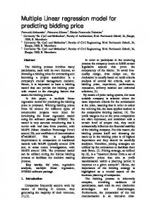
The proof of the theorem is completed by taking expectation on M3 [(βˆ1PTE (d))|τ ] with respect to τ . Figure 1, displays the behavior of the mse based relative efficiency functions of the SE and SPTE for a fixed α with the change in the value of ∆2 . The four graphs illustrate the different features of the relative efficiency functions for selected values of the coefficient of distrust, d = 0.00, 0.25, 0.50, 1.00 when ν is fixed at 5. Figure 2, displays the behavior of the mse based relative efficiency functions of the SE and SPTE for a fixed α with the change in the value of ∆2 . The four graphs illustrate the different features of the relative efficiency functions for selected values of the degrees of freedom, ν = 5, 10, 20, 40 when d is fixed at 0.50. Some Properties of the MSE of SPTE (a) Under the null hypothesis ∆2 = 0, and hence the mse of βˆ1PTE (d) equals µ
·
1 σ∗2 1 − (1 − d2 )G∗3,m Fα ; 0 Sxx 3
¶¸
. Sxx 1−d
≥
9
(5.16)
On the other hand, (5.9) may be rewritten as ³1 ´ ³1 ´i σ∗2 h 1 + (1 − d)G∗3,m Fα ; ∆∗ {2∆2 − (1 + d)} − (1 − d2 )G∗5,m Fα ; ∆∗ Sxx 3 5
≤
(5.17)
σ∗2 1+d whenever ∆2 < . Sxx 2
(5.18)
This means that the mse of βˆ1PTE (d) as a function of ∆2 crosses the constant line M1 (β˜1 ) = ³
σ∗2 Sxx
in the interval
1+d 1+d 2 , 1−d
´
.
(d) A general picture of the mse graph may be described as follows: The mse-function begins with the smallest value
σ∗2 Sxx
h
1 − (1 − d2 )G∗3,m
³
1 3 Fα ; 0
´i
at ∆2 = 0. As ∆2 grows
large, the function increases monotonically crossing the constant line
³
´
1+d 1+d 2 , 1−d and reaches a maximum 2 ∗ towards Sσxx as ∆2 → ∞.
5.3
³
in the interval
1+d 1−d , ∞
´
σ∗2 Sxx
in the interval
then monotonically decreases
The Bias and MSE of SE
Following Balforine and Zacks (1992) we compute the bias and the mse of the SE, βˆ1S . Theorem 5.3: For the Student-t regression model the bias of the SE of the slope is given by
−σ cKn {2Φ(∆) − 1}, B4 (βˆ1S ) = √ Sxx q
where Kn =
(5.19)
Γ( n−1 ) 2 2 n−2 Γ( n−2 ) . 2
Proof: Conditional on τ , the bias of the SE is defined by "
E[βˆ1S
where Z =
√ Sxx (β˜1 −β10 ) τ
Sn (β˜1 − β10 ) − β1 ] = −cE √ | Sxx (β˜1 − β10 )| ½ ¾ c Z = −√ E[Sn ]E , |Z| Sxx
#
(5.20)
n
∼ N (∆τ , 1). We use the following lemma to evaluate E
Z |Z|
o
.
Lemma 5.3. If Z ∼ N (Λ, 1) and φ(Z 2 ) is a Borel measurable function, then ½
E
Z |Z|
¾
= 1 − 2Φ(−Λ)
(5.21)
where Φ(·) is the c.d.f. of the standard normal distribution. The proof of the lemma is q 2 2 Γ(n−1) straightforward. Note that conditional on τ , mSn ∼ χ2 and hence E[S ] = τ. τ2
m
So, for a given τ , the bias of the SE becomes c B4 (βˆ1S |τ ) = − √ Kn τ {2Φ(∆τ ) − 1}. Sxx
10
n
n−2 Γ( n−2 ) 2
(5.22)
Expectation of B4 (βˆ1S |τ ) with respect to τ completes the proof. From the expression of the bias function, the quadratic bias of the SE, QB4 (βˆS ) is obtained as 1
QB4 (βˆ1S ) =
σ2 2 2 c Kn {2Φ(∆) − 1}2 . Sxx
(5.23)
2 ∗ As ∆2 → 0, QB4 (βˆ1S ) → 0 and as ∆2 → ∞, QB4 (βˆ1 S ) → Sσxx Kn2 c2 . Therefore, QB4 (βˆ1S ) is a non-decreasing monotonic function of ∆2 . Thus, unless ∆2 is near the
origin, the quadratic bias of the SE is significantly large. Theorem 5.4: For the Student-t regression model the mse of the SE of the slope is given by
where η(∆∗ ) =
Γ( ν−1 ) 2 Γ( ν2 )
³
h io σ2 n 2 M4 (βˆ1S ) = ∗ 1 − Kn2 2η(∆∗ ) − 1 , Sxx π
1+
∆∗ ν−2
´− ν
2
Proof: From the definition, conditional on τ , the mse of βˆ1S is (
E[(βˆ1S − β1 )2 |τ ] = E(β˜1 − β1 )2 + c2 E(Sn2 )E
τ2 Sxx
(β˜1 − β10 )2 √ [ Sxx (β˜1 − β10 )]2
)
(5.25)
¾ ½ ˜ (β1 − β1 )(β˜1 − β10 )
E(Sn ) √ | Sxx (β˜1 − β10 )| ³ Z ´o c2 τ 2 τ 2 Kn n + − 2c E(|Z|) − ∆τ E , Sxx Sxx |Z|
−2cE =
(5.24)
where Z ∼ N (∆τ , 1). To find E(|Z|), we have the following lemma. Lemma 5.4. If Z ∼ N (Λ, 1), then r
E(|Z|) =
2 −Λ2 /2 e + Λ{2Φ(Λ) − 1} π
(5.26)
where Φ(·) is the c.d.f. of the standard normal variable. See Khan and Saleh (2001) for the proof of the above theorem. Therefore, the mse of βˆ1S is given by ½
τ2 1 + c2 − 2cKn M4 (βˆ1 S ) = Sxx
r
¾
2 −∆2τ /2 e . π
(5.27)
The value of c which minimizes (5.27) depends on ∆2τ and is given by r
∗
c =
2 2 Kn e−∆τ /2 . π
To make c∗ independent of ∆2τ , we choose c0 = to
q
2 π Kn .
(5.28) Thus, optimum M4 (βˆ1S ) reduces
h io τ2 n 2 2 M4 (βˆ1S ) = 1 − Kn2 2e−∆τ /2 − 1 . (5.29) Sxx π Expectation·of the¸ above expression with respect to τ completes the proof. Note that ³ ´− ν ∆2 τ Γ( ν−1 ) 2 ∆∗ 2 1 + ν−2 η(∆∗ ) = Eτ e− 2 = Γ(ν) .
11
6
Comparative Study
In this Section we compare the bias of the three estimators. Also, we define the relative efficiency functions of the estimators, and analyze these functions to compare the relative performances of the estimators.
6.1
Comparing Quadratic Bias Functions
First, we note that the quadratic bias of the RE, SPTE and SE are given by QB2 [βˆ1 (d)] = QB3 [βˆ1PTE (d)] = QB4 [βˆ1S ] =
σ∗2 (1 − d)2 ∆2 Sxx ½ ³1 ´¾2 σ∗2 (1 − d)2 ∆2 G∗3,m Fα ; ∆∗ Sxx 3 2 σ∗ 2 2 c Kn {2Φ(∆) − 1}2 . Sxx
(6.1)
Clearly, under the null-hypothesis QB2 [βˆ1 (d)] = QB3 [βˆ1PTE (d)] = QB4 [βˆ1S (d)] = 0 for all d and α. When ∆ → ∞, QB2 [βˆ1 (d)] → ∞ except at d = 1; QB3 [βˆ1PTE (d)] → 0 for all α and 2 ∗ 2 c Kn2 , a constant that does not depend on d. Therefore, in terms d; and QB4 [βˆ1 S ] → Sσxx of quadratic bias, RE is uniformly dominated by both the SPTE and SE. For very large values of ∆, the SE is dominated by the SPTE regardless of the value of α. From small to moderate values of ∆, there is no uniform domination of one estimator over the other. In this case, domination depends on the level of significance, α. For small values of α, the SPTE is dominated by the SE and for larger values of α, the SE is dominated by the SPTE. However, Chiou and Saleh (2002) suggest the value of α to be between 20% and 25%. In this interval of α, the quadratic bias of the SPTE approaches to zero for not too small values of ∆. However, in practice, the non-centrality parameter is unlikely to be very large (otherwise the credibility of prior information is in serious question) and α is usually preferred to be small. The quadratic bias of the SE is relatively stable and approaches to a constant value starting from some moderate value of ∆ and is unaffected by the choice of d and α. Therefore, the SE may be a better choice among the biased estimators considered in this paper.
6.2
The Relative Efficiency
First we define the relative efficiency functions of the biased estimators as the ratio of the reciprocal of the mse functions. Then we compare the relative performance of the estimators by using the relative efficiency criterion. 12
Comparing RE against UE The relative efficiency of βˆ1 (d) compared to β˜1 is denoted by RE[βˆ1 (d) : β˜1 ] and is obtained as RE[βˆ1 (d) : β˜1 ] = [d2 + (1 − d)2 ∆2 ]−1 .
(6.2)
We observe the following based on (6.2). (i) If the non-sampling information is correct, i.e., ∆2 = 0, the RE[βˆ1 (d) : β˜1 ] = d−2 > 1 and βˆ1 (d) is more efficient than β˜1 . Thus, under the null hypothesis the biased estimator, RE performs better than the unbiased estimator, UE. (ii) If the non-sampling information is incorrect, i.e., ∆2 > 0 we study the expression in (6.2) as a function of ∆2 for a fixed d-value. As a function of ∆2 , (6.2) is a decreasing function with its maximum value d−2 (> 1) at ∆2 = 0 and minimum value 0 at ∆2 = +∞. It equals 1 at ∆2 = 1+d . Thus, if ∆2 ∈ [0, 1+d ), βˆ1 (d) is more efficient than β˜1 , and 1−d
1−d
outside this interval β˜1 is more efficient than βˆ1 (d). For example, if d = 21 , the interval in which βˆ1 (d) is more efficient than β˜1 is [0, 3), while β˜1 is more efficient in [3, ∞) than βˆ1 (d). For d= 0.5 the maximum efficiency of βˆ1 (d) over β˜1 is 4. Comparing SPTE against UE Now, we consider the relative efficiency of the SPTE compared to the UE. It is given by RE[βˆ1PTE (d) : β˜1 ] =
h
1 − (1 − d2 )G∗3,m n
× 2G∗3,m
³1
3
³1
3
´
Fα ; ∆∗ + (1 − d)∆2
´
Fα ; ∆∗ − (1 + d)G∗5,m
³1
5
Fα ; ∆∗
(6.3) ´oi−1
for any fixed d (0 ≤ d ≤ 1) and at a fixed level of significance α. As Fα → ∞, RE[βˆ1PTE (d) : β˜1 ] → [1 − (1 − d2 ) + (1 − d)2 ∆2 ]−1 = [d2 + (1 − d)2 ∆2 ]−1 which is the relative efficiency of βˆ1 (d) compared to β˜1 . On the other hand, as Fα → 0, RE[βˆ1PTE (d) : β˜1 ] → 1. This means the relative efficiency of the SPTE is the same as the unrestricted estimator, β˜1 . Note that under the null hypothesis, ∆2 = 0, the relative efficiency expression (6.3) equals h
1 − (1 − d2 )G∗3,m
³1
3
Fα ; 0
´i−1
≥ 1,
(6.4)
which is the maximum value of the relative efficiency. Thus the relative efficiency function monotonically decreases crossing the 1-line for ∆2 -value between
1+d 2
and
1+d 1−d ,
to a
minimum for some ∆2 = ∆2min and then monotonically increases, to approach the unit value from below. The relative efficiency of the preliminary test estimator equals unity whenever the value of ∆2 is (1 + d)
∆2∗ = ½
G∗
( 1 Fα ;∆∗ )
5 2 − (1 + d) G5,m ∗ (1F 3,m 3
13
α ;∆
∗)
¾,
(6.5)
where ∆2∗ lies in the interval
³
1+d 1+d 2 , 1−d
´
. This means that
i
h
< < RE βˆ1PTE (d) : β˜1 = 1 according as ∆2∗ = ∆2 . >
(6.6)
>
Finally, as ∆2 → ∞, RE[βˆ1PTE (d) : β˜1 ] → 1. Thus, the preliminary test estimator is more efficient than the unrestricted estimator whenever ∆2 < ∆2 , otherwise β˜1 is more ∗
efficient than SPTE up to a moderate value of compared to βˆ1 (d) we have
∆2 .
As for the relative efficiency of βˆ1PTE (d)
i
h
RE βˆ1PTE (d) : βˆ1 = [d2 + (1 − d)2 ∆2 ][1 + g(∆2 )]−1 ,
(6.7)
where ½
g(∆2 ) = (1 − d)∆2 2G∗3,m
³
1 ∗ 3 Fα ; ∆
´
− (1 + d)G∗5,m
−(1 + d2 )G∗3,m
³
1 ∗ 3 Fα ; ∆
´
³
1 ∗ 5 Fα ; ∆
´¾
.
(6.8)
Under the null-hypothesis, h ³1 ´i−1 RE[βˆ1PTE (d) : βˆ1 (d)] = d2 1 − (1 − d2 )G∗3,m Fα ; 0 ≥ d2 . 3
(6.9)
At the same time we consider the result at (6.3). In combination, we obtain d2 ≤ RE[βˆ1PTE (d) : βˆ1 (d)] ≤ 1 ≤ RE[βˆ1PTE (d) : β˜1 ].
(6.10)
For general ∆2 > 0, we have < RE[βˆ1PTE (d) : βˆ1 (d)] = 1 according as >
n
³
(6.11)
´o
1 − G∗3,m 13 Fα ; ∆∗ < 1+d n ³ ´ ´o . ³ ∆2 = > 1−d 1 − 2G∗3,m 13 Fα ; ∆∗ − (1 + d)G∗5,m 15 Fα ; ∆∗
(6.12)
Finally, as ∆2 → ∞, RE[βˆ1PTE (d); βˆ1 (d)] → 0. Thus, except for a small interval around 0, βˆPTE (d) is more efficient than βˆ1 (d). 1
Comparing SE against UE The relative efficiency of βˆ1S compared to β˜1 is given by h
RE(βˆ1S : β˜1 ) = 1 −
oi−1 2 2 n −∆2 /2 Kn 2e −1 . π
(6.13)
Under the null-hypothesis ∆2 = 0, and hence h 2 i−1 RE(βˆ1S : β˜1 ) = 1 − K2n ≥ 1. π
14
(6.14)
Relative efficiencies for d=0, ν=[5.00], α=[0.05] and n=20
Relative efficiencies for d=0.25, ν=[5.00], α=[0.05] and n=20
5
5 UE RE SE SPTE
4 Relative efficiency
Relative efficiency
4 3 2 1 0
UE RE SE SPTE
3 2 1
0
5
10 ∆
15
0
20
0
Relative efficiencies for d=0.5, ν=[5.00], α=[0.05] and n=20
∆
15
20
1.6 UE RE SE SPTE
3
UE RE SE SPTE
1.4 Relative efficiency
Relative efficiency
10
Relative efficiencies for d=1, ν=[5.00], α=[0.05] and n=20
4
2
1
0
5
1.2 1 0.8
0
5
10 ∆
15
0.6
20
0
5
10 ∆
15
20
Figure 1: Graph of relative efficiency of RE, SPTE and SE relative to UE for ν = 5 and different d In general, RE(βˆ1S : β˜1 ) decreases from [1 − π2 Kn2 ]−1 at ∆2 = 0 and crosses the 1-line at ∆2 = ln 4 and then goes to the minimum value h
1+
2 2 i−1 K π n
as ∆2 → ∞.
(6.15)
Thus, the loss of efficiency of βˆ1S relative to β˜1 is h
1− 1+ while the gain in efficiency is
h
1−
2 2 i−1 K π n
2 2 i−1 K π n
(6.16)
(6.17)
respectively which is achieved at ∆2 = 0. Thus, for ∆2 < ln 4, βˆ1S performs better than β˜1 , otherwise β˜1 performs better. The property of βˆ1S is similar to the preliminary test estimator but does not depend on the level of significance. As ∆2 → ∞ the relative 15
Relative efficiencies for d=0.5, ν=[5.00], α=[0.15] and n=20
Relative efficiencies for d=0.5, ν=[10.00], α=[0.15] and n=20 4
UE RE SE SPTE
3
Relative efficiency
Relative efficiency
4
2
1
0
UE RE SE SPTE
3
2
1
0
5
10 ∆
15
0
20
0
Relative efficiencies for d=0.5, ν=[20.00], α=[0.15] and n=20
∆
15
20
4 UE RE SE SPTE
3
Relative efficiency
Relative efficiency
10
Relative efficiencies for d=0.5, ν=[40.00], α=[0.15] and n=20
4
2
1
0
5
UE RE SE SPTE
3
2
1
0
5
10 ∆
15
0
20
0
5
10 ∆
15
20
Figure 2: Graph of relative efficiency of RE, SPTE and SE relative to UE for d = 0.5 and different ν efficiency of SPTE with respect to UE approaches to 1 and that of the SE with respect to h
UE approaches to 1 + π2 Kn2
i−1
.
Comparing efficiency of SE relative to SPTE The maximum relative efficiency of the SE relative to SPTE attained for ∆ = 0 and d = 1, regardless of the value of α. At ∆ = 0, as the coefficient of distrust, d decreases, the relative efficiency of SE also decreases, and it decreases below 1 for d = 0. Starting from some moderate value of ∆, relative efficiency of SE becomes less than 1 and converges to a stable value, below one, as ∆ → ∞. Except for ∆ = 0 and near 0 the relative efficiency of SE is always higher for smaller values of d than larger values of d, before converging to a stable value. The difference between the relative efficiencies of SE for different values of d is higher for lower value of α then it’s higher values. As α increases this difference decreases. Moreover, as α increases, the relative efficiency of SE also increases for ∆ = 0 16
or near 0.
7
Concluding Remarks
The UE is based on the sample data alone and it is the only unbiased estimator among the four estimators considered in this paper. The introduction of the non-sample information in the estimation process causes the estimators to be biased. However, the biased estimators perform better than the unbiased estimator when they are judged based on the mse criterion. The performance of the biased estimators depend on the value of the departure parameter ∆. In case of the SPTE, the performance also depends on the value of the level of significance. Under the null hypothesis, the departure parameter is zero, and the SE dominates all other estimators if α is not too high. As α increases, the performance of the SPTE improves when ∆ is not too close to zero. At a lower level of significance, the SE performs better than the SPTE more often and over a wider range of values of ∆. When the value of ∆ is not far from 0, the SE always over performs the SPTE and RE. Therefore, in practice if the researcher could gather a value of β1 from the prior knowledge or experience that is not too far from its true value, the SE would be the best choice as an ‘improved’ estimator of the slope. ACKNOWLEDGEMENTS The authors thankfully acknowledge some valuable suggestions of two unknown reviewers that have contributed to the improvement of the quality and presentation of the paper.
References Anderson, T.W. (1993). Nonnormal multivariate distributions: Inference based on elliptically contoured distributions. In Multivariate Analysis: Future Directions. ed by C.R. Rao. North-Holland, Amsterdam, 1–24. Bancroft, T.A. (1944). On biases in estimation due to the use of the preliminary tests of significance. Ann. Math. Statist., 15, 190–204. Bolfarine, H. and Zacks, S. (1992). Prediction Theory for Finite Populations. SpringerVerlag, New York. Box, G.E.P. and Tiao, G.C. (1992). Bayesian Inference in Statistical Analysis. Wiley, New York. Celler, D., Fourdriunier, D and Strawderman, W.E. (1995). Shrinkage positive rule estimators for spherically symmetric distributions. Journal of Multivariate Analysis, 53, 194-209. Chmielewski, M.A. (1981). Elliptically symmetric distributions. International Statistical Review, Vol. 49, 67–74. Chiou, P. and Saleh, A.K.Md.E. (2002). Preliminary test confidence sets for the mean of a multivariate normal distribution. Journal of Propagation in Probability and Statistics, 2, 177-189. 17
Fang, K.T. and Anderson, T.W. (1990). Statistical Inference in Elliptically Contoured and Related Distributions. Allerton Press Inc., New York. Fang, K.T. and Zhang, Y. (1990). Generalized Multivariate Analysis, Science Press and Springer-Verlag, New York Fisher, R.A. (1956). Statistical Methods in Scientific Inference. Oliver and Boyd, London. Fisher, R.A. (1960). The Design of Experiments. 7th ed., Hafner, New York. Fraser, D.A.S. and Fick, G.H. (1975). Necessary analysis and its implementation. In Proc. Symposium on Statistics and Related Topics. ed. by A.K. Md. E. Saleh, Carleton University, Canada, 5.01–5.30. Fraser, D.A.S. (1979). Inference and Linear Models, McGraw–Hill, New York. Giles, J.A. (1991). Pre-testing for linear restrictions model with spherically symmetric disturbances. Journal of Econometrics, Vol. 50, 377–398. Han, C.P. an Bancroft, T.A. (1968). On pooling means when variance is unknown. Jou. Amer. Statist. Assoc., 63, 1333-1342. James, W. and Stein, C. (1961). Estimation with quadratic loss. Proceedings of the Fourth Berkeley Symposium on Mathematical Statistics and Probability. Berkeley, California, 361–379. Judge, G.C. and Bock, M.E. (1978). Statistical Implications of Pre-test and Stein-rule Estimators in Econometrics. North Holland, Amsterdam. Khan, S. (1997). Likelihood based inference on the mean vectors of two multivariate Student-t populations. Far East Journal of Theoretical Statistics. 1, 1-17. Khan, S. and Haq, M.S. (1990). Prediction distribution for the linear model with multivariate Student-t error. Communications in Statistics: Theory & Methods, Vol. 19, 4705–4712. Khan, S. and Saleh, A.K.Md.E. (1997). Shrinkage pre-test estimator of the intercept parameter for a regression model with multivariate Student-t errors. Biometrical Journal. Vol. 39, 131–147. Khan, S. and Saleh, A.K.Md.E. (1998). Comparison of estimators of the mean based on p-samples from multivariate Student-t population. Communications in Statistics: Theory & Methods. Vol. 27(1), 193-210. Khan, S. and Saleh, A.K.Md.E. (2001). On the comparison of the pre-test and shrinkage estimators for the univariate normal mean. Statistical Papers, 42(4), 451-473. Lange, K.L. Little, R.J.A., and Taylor, J.M.G. (1989). Robust statistical modeling using the t-distribution. Journal of American Statistical Association, Vol. 84, 881–896. Lobato, I. N. (2001). Testing That a Dependent Process Is Uncorrelated, Journal of the American Statistical Association, Volume 96(455), 1066-1076(11). Maatta, J.M. and Casella, G. (1990). Developments indecision-theoretic variance estimation, Statistical Sciences, Vol. 5, 90–101. Prucha I.R. and Kelegian, H.H. (1984). The structure of simultaneous equation estimators: A generalization towards non-normal disturbances, Econometrica, Vol. 52, 721–736. Saleh, A K Md E. (2006). Theory of Preliminary Test and Stein-Type Estimation with Applications. Wiley, New York. Saleh, A.K.Md.E. and Sen, P.K. (1978). Non-parametric estimation of location parameter after a preliminary test on regression. Annals of Statistics, 6, 154-168. Sclove, S.L., Morris, C. and Radhakrishnan, R. (1972). Non-optimality of preliminary-test estimators for the mean of a multivariate normal distribution. Ann. Math. Statist., Vol. 43, 1481–1490. Sen, P.K and Saleh, A.K.Md.E. (1985). On some shrinkage estimators of multivariate location. Annals of Statistics. 13, 272-281. Singh, R.S. (1988). Estimation of error variance in linear regression models with errors having multivariate Student-t distribution with unknown degrees of freedom. Economics Letters, Vol. 27, 47–53. Spanos, A. (1994). On modeling heteroskedasticity: The Student’s t and elliptical linear regression models. Econometric Theory, Vol. 10, 286–315. 18
Stein, C. (1956). Inadmissibility of the usual estimator for the mean of a multivariate normal distribution. Proceedings of the Third Berkeley Symposium on Math. Statist. and Probability, University of California Press, Berkeley, Vol. 1, 197-206. Stein, C. (1981). Estimation of the mean of a multivariate normal distribution. Ann. Statist. 9, 1135–1151. Ullah, A. and Walsh, V.Z. (1984). On the robustness of LM, LR and W tests in regression models. Econometrica, Vol. 52, 1055–1066. Zellner, A. (1976). Bayesian and non-Bayesian analysis of the regression model with multivariate Student-t error term. Journal of American Statistical Association, Vol. 66, 601–616.
19