For convenience, let d0 = 0 and sp+1 = 1. Zero-order jumps (m ..... Flag the design points ftij; j = 1;2;. ; n1g where tij ... rst-order derivative for convenience. As we ...
A LOCAL POLYNOMIAL JUMP DETECTION ALGORITHM IN NONPARAMETRIC REGRESSION Peihua Qiu Biostatistics Program The Ohio State University M200 Starling Loving Hall 320 West 10th Avenue Columbus, OH 43210-1240
Brian Yandell Department of Statistics University of Wisconsin - Madison 1210 West Dayton Street Madison, WI 53706
Abstract We suggest a one dimensional jump detection algorithm based on local polynomial tting for jumps in regression functions (zero-order jumps) or jumps in derivatives ( rst-order or higherorder jumps). If jumps exist in the m-th order derivative of the underlying regression function, then an (m + 1) order polynomial is tted in a neighborhood of each design point. We then characterize the jump information in the coe�cients of the highest order terms of the tted polynomials and suggest an algorithm for jump detection. This method is introduced brie y for the general set-up and then presented in detail for zero-order and rst-order jumps. Several simulation examples are discussed. We apply this method to the Bombay (India) sea-level pressure data.
Key Words: Nonparametric jump regression model, Jump detection algorithm, Least squares line, Threshold value, Modi cation procedure, Image processing, Edge detection.
1 Introduction Stock market prices often jump up or down under the in uence of some important random events. Physiological response to stimuli can likewise jump after physical or chemical shocks. Regression functions with jumps may be more appropriate than continuous regression models for such data. The one dimensional (1-D) nonparametric jump regression model (NJRM) with jumps in the m-th derivative can be expressed as
Yi = f (ti ) + �i; i = 1; 2; � � �; n; 1
(1.1)
f
p m) (t) = g(t) + X di I [si ;si+1 ) (t); i=1
(1.2)
(
with design points 0 � t1 < t2 < � � � < tn � 1 and iid errors f�i g having mean zero and unknown variance �2 . The m-th order derivative f (m) (t) of the regression function f (t) consists of a continuous part g(t) and p jumps at positions fsi ; i = 1; 2; � � � ; pg with magnitudes fdi ? di?1 ; i = 1; 2; � � � ; pg. For convenience, let d0 = 0 and sp+1 = 1. Zero-order jumps (m = 0) in the regression function itself correspond to the step edge in image processing. First-order jumps (m = 1) may exist in the rst derivative of f (t), related to the roof edge in image processing. For m > 1, the jumps in (1.2) are called higher-order. The objective of this paper is to develop an algorithm to detect the jumps of 1-D NJRM (1.1)-(1.2) from the noisy observations fYi ; i = 1; 2; � � � ; ng.
Example 1.1 (Bombay sea-level pressure data) Figure 1.1 shows a sea-level presure data
which was provided by Dr. Wilbur Spangler at National Center for Atmospheric Research (NCAR), Boulder, Colorado. The small dots represent the December sea-level pressures during 1921-1992 in Bombay, India. Shea et al. (1994) pointed out that \a discontinuity is clearly evident around 1960. : : : Some procedure should be used to adjust for the continuity". By usng the procedure introduced in this paper, a jump is detected. The tted model with this detected jump accommodated is shown in the plot by the solid curves. As a comparison, we plot the tted model with the usual kernel smoothing method by the dotted curve. More explanation about this example is given in Section 4.3. 1017
. .
1015 1013
PRESSURE
. .. . .
..
.. . .
.
. . . . . .. . . . . . . . . . . . . .. . . ..
. . . . . .. . ... . ... . . . .. . .. . . . . . .
.
1011
.. 1920
1940
1960 YEAR
.
1980
Figure 1.1: The December sea-level pressures during 1921-1992 in Bombay, India. The solid curves represent the t from our jump-preserving algorithm. The dotted curve is the usual kernel smoothing t without considering the jump structure. 2
McDonald and Owen (1986) proposed an algorithm based on three smoothed estimates of the regression function, corresponding to the observations on the right, left, and both sides of a point in question, respectively. They then constructed a \split linear smoother" as a weighted average of these three estimates, with weights determined by the goodness-of- t values of the estimates. If there was a jump near the given point, then only some of these three estimates provided good ts, accommodating the discontinuities of the regression functions. Hall and Titterington (1992) suggested an alternative method by establishing some relations among three local linear smoothers and using them to detect the jumps. This latter method is easier to implement. Related research on this topic includes kernel-type methods for jump detection in Muller (1992), Qiu (1991,1994), Qiu et al (1991), Wu and Chu (1993), Yin (1988), etc. These methods were based on the di�erence between two one-sided kernel smoothers. Wahba (1986), Shiau (1987) and several others regarded the NJRMs as partial linear regression models and tted them with partial splines. More recently, Eubank and Speckman (1994) and Speckman (1993) treated the NJRM (1.1)-(1.2) as a semi-parametric regression model and proposed estimates of the jump locations and magnitudes. Loader (1994) suggested a jump detector based on local polynomial kernel estimators. In this paper, we suggest an alternative method. At a given design point ti , we consider its neighborhood N (ti ) := fti?` ; ti+1?` ; � � � ; ti ; � � � ; ti?1+` ; ti+` g with width k = 2` + 1 � n an odd positive integer, for ` + 1 � i � n ? `. We then t a local polynomial function of order (m + 1) by the least squares (LS) method in that neighborhood, which can be expressed as
Y^ (i) (t) = ^0(i) + ^1(i) t + � � � + ^m(i)+1 tm+1 ; t 2 N (ti ); i = ` + 1; � � � ; n ? `:
(1.3)
Intuitively, if f (m) (t) is smooth at ti , then ^m(i)+1 is close to f (m+1) (ti ) for large enough n. If f (m) (t) ) has a jump at ti , however, f ^m(j+1 gjn=?``+1 has an abrupt change at ^m(i)+1 . Hence, these coe�cients carry information about both the continuous and the jump components of f (m) (t) (given in (1.2)). A jump detection criterion can be formed which excludes the information about the continuous part but preserves the jump information. An important feature of such algorithm is that it is easy to implement. From the above brief description, this algorithm is based on estimated LS coe�cients which are available from all statistical softwares. Its computation complexity is O(n). Another feature of this method is that it does not require the number of jumps to be known beforehand as most existing methods did. Jumps are automatically accommodated with our jump preserving curve tting procedure. 3
We should point out that in our algorithm the window width k is still unde ned. How should one choose a proper window width in practice ? This is a common problem in local smoothing methods. In some applications, people have used a visual intuitive method to adjust the window width. Hastie and Tibshirani (1987) suggested using 10-50% observations for each running lines smoother in their local scoring algorithm. Stone (1977) suggested the cross-validation method to choose the window width. For more discussions on the selection of the window width, please refer to Chapter 6 in Hardle (1991). In most applications, we are interested in checking for jumps in the regression function itself or in its rst-order derivative. Hence in the following sections, we concentrate on these two special cases. In Section 2, a jump detection criterion for the case of m = 0 is derived, with a corresponding algorithm. Jump detection in slope is discussed in Section 3. In Section 4, some simulation results are presented. We return to the Bombay (India) sea-level pressure data in Section 4.3. Our method is compared with some kernel-type methods in Section 5. We conclude the article with some remarks in Section 6. Some supporting materials are given in the Appendix. At the end of this section, we want to point out that the 2-D version of the current problem (namely, jump detection in surfaces) is closely related to edge detection in image processing. We refer the interested readers to Besag et al. (1995), Gonzalez and Woods (1992), Qiu and Bhandarkar (1996), Qiu and Yandell (1997) and the references cited there.
2 Jump Detection in the Regression Functions In this section we discuss the jump detection in the regression function itself. This corresponds to m = 0 in model (1.1)-(1.2). For simplicity of presentation, we assume that the design points are equally spaced over [0,1]. Most of the derivation of the jump detection criterion presented below is intuitive, although mathematically rigorous arguments are available. Based on the derived criterion, we suggest a jump detection algorithm at the end. As we introduced in Section 1, we t a least squares line
Y^ (i) (t) = ^0(i) + ^1(i) t; t 2 N (ti ) in a neighbourhood N (ti ) at any design point ti , for ` + 1 � i � n ? `. Throughout this paper we make the following assumption (AS1) on the NJRM of equations (1.1)-(1.2). 4
(AS1) Only one jump is possible in any neighbourhood N (ti ). If ti is a jump point, then no other jumps exist in N (ti?k ) [ N (ti ) [ N (ti k ). +
Remark 2.1 Assumption (AS1) implies that jump locations are not very close to each other. Al-
ternatively, there is enough data (n large, k=n small) to distinguish nearby jumps. This assumption seems to be reasonable in many applications. In Appendix A we present a theorem (Theorem A.1) which gives some properties of ^1(i) . By that theorem, ^1(i) � B1 (ti ) := g0 (ti ) when there is no jump in N (ti ); and
^1(i) � B1 (ti ) := g+0 (ti ) + h1 (r)C0 ? (r)C1 if a jump exists in N (ti ) and the jump location is at ti?`+r ; 0 � r � 2`, where \�" means that noise in the data and a high order term are ignored, C0 and C1 are the jump magnitudes of f (t) and its rst order derivative at the jump location, (r) is a positive function taking values between 0 and 1, h1 (r) := k(6knr+1) (1 ? k?r 1 )C0 and g+0 (ti ) = g0 (ti ) if r 6= `.
Remark 2.2 We want to point out that some quantities used in this paper such as k; ^ i and ( ) 1
h1 (r) all depend on n. We did not make this explicit in notations for simplicity. Their meaning should be clear from contexture introduction.
Example 2.1 Let f (t) = 5t + I : ; (t). Consider a sample of size 100 and let k be 7. Then ^ i � B (ti ) = 10ti + If: �ti �: g : : �?: ti (1 ? : : ?ti ); 4 � i � 97. fB (ti ); 4 � i � 97g is shown in 2
( ) 1
1
Figure 2.1(a).
47
[0 5 1]
6( 53 ) 53 ( 07) ( 08)
53 06
1
From Figure 2.1(a) and Theorem A.1 in Appendix A, we can see that f ^1(i) g carries useful information about the jumps. This information is mainly in the \jump factor" h1 (r)C0 of B1 (ti ). k?1) = O(n=k) which tends to in nity with n. If we h1 (r) has a maximum value at r = ` of 1:k5(nk(+1) have prior information about the bound of the \continuous factor" g0 (ti ) (in the case ti is not a jump point), then those points could be agged as jump points if their LS slopes are bigger than the prior bound. However, that prior bound may not be available in many applications. Our strategy to overcome this di�culty is to nd an operator to remove the continuous factor from B1 (ti ) and to preserve its jump factor at the same time. Notice that the continuous factors g0 (ti ) and g0 (tj ) are close to each other when ti and tj are close. Therefore, a di�erence-type operator can remove the continuous factor. When ti and tj are far enough apart such that only one of B1 (ti ) and B1 (tj ) can have a jump factor, the di�erence between B1 (ti ) and B1 (tj ) preserves the jump factor. Many 5
15 10
20
5
15
0
10
-5
5 0
0.25
0.50
0.75
1.00
0.25
(a) position t
0.50
0.75
(b) position t
Figure 2.1: If f (t) = 5t2 + I[0:5;1](t), n = 100; k = 7, then ^1(i) � B1 (ti ): fB1 (ti )g consists of both the continuous and the jump factors. It is shown in plot (a) by the \diamond" points. After using the di�erence operator de ned in (2.1), fJ1 (ti )g consists mainly of the jump factor. It is shown in plot (b). di�erence-type operators could be found. In this paper, we suggest using the following:
8 >< ^ i ? ^ i?` if j ^ i ? ^ i?` j � j ^ i ? ^ i ` j i � := > i : ^ ? ^ i ` if j ^ i ? ^ i?` j > j ^ i ? ^ i ` j ( ) 1
( ) 1
( 1
)
( ) 1
( 1
)
( ) 1
( + ) 1
( ) 1
( + ) 1
( ) 1
( 1
)
( ) 1
( + ) 1
(2.1)
for k � i � n ? k + 1. That is, use the di�erence of smaller magnitude. By the above intuitive explanations, we can see that
8 >< 0 i � � J (ti ) := > : h (r)C ( ) 1
1
2
0
if there is no jump in N (ti ) if there is a jump at ti?`+r ; 0 � r � k ? 1
(2.2)
where h2 (r) is one of h1 (r) ? h1 (r ? `) and h1 (r) ? h1 (r + `) with smaller magnitude and h1 (j ) = 0 when j < 0 or j > k ? 1.
h2 (r) has the same maximum value as h1 (r). In the case of example 2.1, fJ1 (ti); 7 � i � 94g is
shown in Figure 2.1(b). From (2.2) and Figure 2.1(b), we can see that f�(1i) g does keep the jump information and delete the continuous factors at the same time. Hence it could be used as our jump detection criterion.
6
Remark 2.3 A possible alternative operator to (2.1) is as follows. For k � i � n ? k + 1, de ne ^ i ^ i?` ^ i ^ i ` ^ i ^ i ` ^ i ^ i?` ��i := j ? j( ^ i ? ^ i?` ) + j ^ i ? ^ i ` j( ? ) j ? j + j ? j ��i is a weighted average of ^ i ? ^ i?` and ^ i ? ^ i ` . From Theorem A.1 and Figure 2.1(a), ( )
( )
( + ) 1
( ) 1
( ) 1
( 1
( 1 ( 1
( ) 1 ( ) 1 )
)
( ) 1
( + ) 1
( ) 1
( ) 1 ( + ) 1
( ) 1 ( ) 1
)
( + ) 1
we can check that �(�i) is small when there is no jump in N (ti ). When there is a jump at ti , �(�i) � h1 (`)C0 where C0 is the jump magnitude.
Remark 2.4 The di�erence operator in (2.1) also narrows the regions that contain jump informa-
tion. A jump a�ects ^1(i) if ti is within 2k of that jump point while it a�ects �(1i) when ti is less than k units away. However, we also pay the price for that di�erence operator. The variance of �(1i) is usually bigger than the variance of ^1(i) . Although it does not a�ect much of the jump detection in the sense of large sample theory since both of them converge to zero, it might be important in nite sample cases. In applications, we suggest plotting both f ^1(i) g and f�(1i) g. In many cases the plot of f ^1(i) g could be very helpful to demonstrate the jumps. This can be seen in the real data example (Section 4.3) and in the simulation examples (Sections 4.1 and 4.2) as well. Large values of j�(1i) j indicate possible jumps near ti . If there is no jump in N (ti ), then ^1(i) ? ^1(i?`) is approximately normally distributed with mean zero, since it is a linear combination of the observations. From (2.1), P (j�(1i) j > u1i ) � P (j ^1(i) ? ^1(i?`) j > u1i ) for any u1i > 0. Therefore consider the threshold value u1i = Z�n =2 �(i) , with �(i) =SD of ^1(i) ? ^1(i?`) . Clearly, �(i)
is independent of i. After some calculations, we have �(i) = nk choice of the threshold value is s n u1 = �^ Z�n =2 k 6(5k2k??13) ;
q
k?3) k2 ?1 �.
6(5
Therefore a natural (2.3)
where �^ is a consistent estimate of �.
The design points ftij : j�1(ij ) j > u1 ; j = 1; 2; � � � ; n1 g can be agged as candidate jump positions. If tij is agged, then its neighboring design points will be agged with high probability. Therefore we need to cancel some of the candidates in ftij ; j = 1; 2; � � � ; n1 g. We do this by the following modi cation procedure which was rst suggested by Qiu (1994).
Modi cation Procedure: For ftij ; j = 1; 2; � � � ; n g, if there are r < r such that the increments of the sequence ir1 < � � � < ir2 are all less than the window width k but ir1 ? ir1 ? > k and ir2 ? ir2 > k, then we say that ftij ; j = r ; r + 1; � � � ; r g forms a tie in ftij ; j = 1; 2; � � � ; n g. 1
1
2
1
+1
1
1
2
1
Select the middle point (tir1 + tir2 )=2 for each tie as a jump position candidate, replacing the tie set 7
in the candidate set ftij ; j = 1; 2; � � � ; n1 g. That is, reduce the candidate set to one representative, the middle point, from each tie set. After the above modi cation procedure, the present candidates include two types of points: those which do not belong to any tie, and the middle points of all of the ties. The jump detection method is summarized in the following algorithm.
The Zero-order Jump Detection Algorithm: 1. For any ti , ` + 1 � i � n ? `, t a least squares line in N (ti ) . 2. Use formula (2.1) to calculate �(1i) ; k � i � n ? k + 1. 3. Use formula (2.3) to calculate the threshold value u1 . 4. Flag the design points ftij ; j = 1; 2; � � � ; n1 g where tij satis es j�1(ij ) j > u1 for j = 1; 2; � � � ; n1 . 5. Use the modi cation procedure to determine the nal candidates set fbi ; i = 1; 2; � � � ; q1 g. Then we conclude that jumps exist at b1 < b2 < � � � < bq1 .
Remark 2.5 The least squares lines tted in step 1 of the above algorithm can be updated easily
from one design point to the next one, since only two points change. Thus the whole algorithm requires O(n) computation. This remark is also true in the general set-up.
Remark 2.6 There is no di�erence for our jump detection whether we t the model (1.3) or t the centered model.
Y^ (i) (t) = ^0(i) + ^1(i) (t ? ti ) + � � � + ^m(i)+1 (t ? ti)m+1 ; t 2 N (ti); i = ` + 1; � � � ; n ? ` In many situations, it is more convenient to use the above model.
Theorem 2.1 Besides the conditions stated in Theorem A.1 in Appendix A, if the con dence level p �n in (2.3) satis es the conditions that (i) limn!1 �n = 0 (ii) limn!1 Z�n = = loglogk = 1 and p 2
(iii) limn!1 Z�n =2 = k = 0, then (1) limn!1 q1 = p; a:s:; and (2) limn!1 bi = si; a:s:; i = 1; 2; � � � ; p. The rate of these convergences is o(n?1 log(n)). (Proof is given in Appendix B.) 8
After we detect the possible jump locations b1 < b2 < � � � < bq1 , the regression function f (t) could be tted separately in intervals f(bi?1 ; bi ); i = 1; 2; � � � ; q1 + 1g where b0 = 0 and bq1 +1 = 1. To t f (t) in each interval (bi?1 ; bi ), we could use either global smoothing method (e.g., the smoothing spline method, Wahba, 1991) or local smoothing method (e.g., the kernel smoothing method, Hardle, 1991; the local polynomial kernel method, Wand and Jones, 1995). By using the kernel smoothing method, \boundary kernels" are necessary in the border regions of the intervials (see e.g., Stone, 1977). When t 2 (bi?1 ; bi ), f^(t) can be de ned as follows. Pn K (t ? t)y ni j j ^ (2.4) f (t) = Pj=1 n K (t ? t) j =1 ni j with Kni (x) = K (x=hn )Ift+x2(bi?1 ;bi )g where K (x) is a kernel function with K (x) = 0 when x 62 [?1; 1] and hn is a parameter related to the window size k by hn = 2kn .
3 Jump Detection in Derivatives Derivatives can be developed in an analogous manner. We consider only the jump detection in the rst-order derivative for convenience. As we introduced in Section 1, we t the following quadratic functions by the least squares method for jump detection.
Y^ (i) (t) = ^0(i) + ^1(i) t + ^2(i) t2 ; t 2 N (ti ); i = ` + 1; � � � ; n ? ` Theorem A.2 in Appendix A gives some properties of ^2(i) . It says that under some regularity conditions ^2(i) � B2 (ti ) := g0 (ti ) when there is no jump in N (ti ), where g(t) is the continuous part of f 0(t). When there is a jump in N (ti ) and the jump location is at ti?`+r ; 0 � r � 2`, then
^2(i) � B2 (ti ) := g+0 (ti ) + h3 (r)C1 ? (r)C2 where C1 and C2 are jump magnitudes of f 0 (t) and its rst order derivative, (r) is a positive function taking values in [0,1], h3 (r) := r(k ? 1 ? r)k[(k12(?ks1)(k??s22))n?3 3r(k ? 1 ? r)] ; 4 2 P sp = ij+=`i?`(tj ? ti )p, p = 2; 4, and g+0 (ti ) = g0 (ti) if r 6= `.
Example 3.1 Let f 0(t) = 5t + I : ; (t). Consider a sample of size 100 and let k be 11. Then ^ i � B (ti ) = 10ti + If: �ti �: g h (100(:55 ? ti )); 6 � i � 95. fB (ti)g is shown in Figure 3.1(a). 2
( ) 2
2
45
[0 5 1]
55
3
2
9
20 15
40
10
30
0
5
20
-5
10 0 0.0
0.25
0.50
0.75
1.00
0.0
(a)
0.25
0.50
0.75
1.00
(b)
Figure 3.1: If f 0(t) = 5t2 + I[0:5;1] (t), n = 100, k is chosen to be 11, then ^2(i) � B2 (ti ). fB2 (ti )g is shown in (a) by the \diamond" points. After using the di�erence operator which is similalar to that in (2.1)-(2.2), we get fJ2 (ti )g which is shown in (b). Similar to (2.1)-(2.2) in Section 2, we construct f�(2i) g from f ^2(i) g and we have fJ2 (ti )g which is shown in Figure 3.1(b) in the case of example 3.1. The threshold value for f�(2i) g is derived in the similar way to u1 , as q k2 s4 ? (k + 1)s22 u2 = �^ Z�n =2 : (3.1) ks ? s2 4
2
The jump detection algorithm in Section 2 can be used here with f�(2i) g and u2 substituting for f�(1i) g and u1 .
4 Numerical Examples 4.1 Jumps in Mean Response We conducted some simulations using the example from Hall and Titterington (1992), which is shown in Figure 4.1. 512 observations fYi g are obtained from f (ti)+ �i for equally spaced ti = i=512, with errors from N (0; �2 ) and � = 0:25. The regression function f (t) = 3 ? 4t when 0 � t � 0:25 ; f (t) = 2 ? 4t when 0:25 < t � 0:5; f (t) = ?1 + 4t when 0:5 < t � 0:75; f (t) = 4 ? 4t when 0:75 < t � 1. f (t) has three jumps, at 0.25, 0.5 and 0.75, and corresponding jump magnitudes of -1,1 and -1, respectively. 10
0
1
y
2
3
We use the zero-order jump detection algorithm to detect the jumps, initially with k = 31. f ^1(i) g is shown in Figure 4.2(a). According to the discussions in section 2, ^1(i) � B1 (ti), including a continuous factor and a jump factor. The jump factor has its e�ect only in the neighborhoods of the jump locations. The continuous factor is negative in intervals 0 � t � 0:25; 0:25 < t � 0:5 and 0:75 < t � 1 and positive in interval 0:5 < t � 0:75. All of these facts can be seen from Figure 4.2(a). We then use operator (2.1) to remove the continuous factors from f ^1(i) g. The remaining jump factors f�(1i) g are shown in Figure 4.2(b). From the graph, we can see that f�(1i) g waves around zero when ti is not in the neighbourhoods of the jumps. This implies that the continuous factor is mostly removed. As we noticed in Remark 2.4, f�(1i) g seems noisier than f ^1(i) g. Figure 4.2(a) reveals the jumps very well in this case since the continuous factor does not contaminate much of the jump information. From the graphs we can approximate the jump positions and k?1) C , where estimate the jump magnitudes from the relationship M � h2 ((k ? 1)=2)C0 = 1:k5(nk(+1) 0 M is the maximum/minimum value of f�(1i) g in the neighborhood of each of the detected jump positions and C0 is the corresponding jump magnitude. For example, in Figure 4.2(b), we can see that there is a jump near 0.75 and M is about -23. Thus the jump magnitude C0 is about k?1) ]?1 M � ?0:99. C0 � [ 1:k5(nk(+1)
0.0
0.25
0.50
0.75
1.00
Figure 4.1: Hall and Titterington functiont f (solid lines) and observations (+). As we noticed in Section 2, if the noise is not took into account, f�(1i) g has a peak with value 1:5n(k ?1) k(k+1) C0 at a jump point with jump magnitude C0 . Comparing with the threshold value in (2.3),
11
20 10
20
0
10 0
-20
-10
-10 -30 0.0
0.25
0.75 (a)
(a) Slope estimates f ^ i
0.25
g (b) Jump information terms f� i
0.50
0.75
(b)
Figure 4.2: g. The dotted lines in plot (b) indicate (+) or (?) threshold value u1 corresponding to Z�n =2 = 3:5. ( ) 1
( ) 1
this jump could be detected if the jump magnitude satis es �^ Z (6(k + 1)(5k ? 3))1=2 : (4.1) C0 > �n =2 1:5(k ? 1)3=2 Although n is not in (4.1), it is actually hidden in k since the above arguments are true only in the case that k=n is small and n is large. (4.1) tells us that (1) if � is bigger (the data is noisier), then only jumps with larger jump magnitudes could be detected; (2) if the con dence level is set higher (�n is small and Z�n =2 is large), then the algorithm is more conservative (jumps with small jump magnitudes would probably be missed); (3) if k is larger (n is also larger), the algorithm could detect jumps with smaller magnitudes or could detect the same jumps with higher con dence level. This last point also implies that to detect the same jump the con dence level could be set a little bit higher when the sample size is larger. In this simulation example, we use n = 512 and k = 31. The peak value of f�(1i) g is about 23.2258. The variance of f�(1i) g is less than 4.0245 (c.f. the derivation of (2.3)). We choose Z�n =2 = 3:5 in the threshold, which corresponds to �n = 0:0004. By (2.3), the threshold value is 14.08 which is smaller than the peak value more than 2 times the variance of f�(1i) g . By (4.1), the algorithm could detect jumps with minimum jump magnitude about 0.6. If k = 49 which is the best width according to Table 4.1 introduced below, then this minimum magnitude could be decreased to about 0.47. 12
0
50
frequency 100
150
1000 independent trials were done, with 963 times to detect 3 jumps, 29 times to detect 2 jumps, 7 times to detect 4 jumps and 1 time to detect only 1 jump. The detected jump locations are shown in Figure 4.3.
0.0
0.25
0.50 location
0.75
1.00
Figure 4.3: Frequency of detected jump locations by the zero-order jump detection algorithm with
n = 512 and k = 31 for 1000 replications.
The choice of k = 31 is somewhat arbitrary. We investigated this with simulations for several n and k values. The results summarized in Figure 4.4 show that if k is chosen very small, some jumps are frequently missed, as the noise of �(1i) swamps the jump information. If k is very large, the wide window width makes the jump information be contaminated by the continuous factors. The corresponding results are not impressive either. The ratios of the \best" window widths (the smallest window widths that give the best results) to the sample sizes have the relations that 35=256 > 49=512 > 79=1024 > 145=2048. This suggests that the ratio of the window size to the sample size should be decreasing as n increases.
4.2 Jump Detection in Slope Some simulation results of jump detection in the rst-order derivative are presented in this part. We also use the example in Hall and Titterington (1992) which is shown in Figure 4.5. 512 observations fYig are obtained from f (ti) + �i for equally spaced ti = i=512, with iid errors from N (0; �2 ) and � = 0:25. f (t) = 3t when 0 � t � 0:5; f (t) = 3 ? 3t when 0:5 < t � 1. It has one rst-order jump at t = 0:5. When k = 121, f ^2(i) g and f�(2i) g are shown in Figure 4.6 (a) and (b) respectively. We performed 13
our simulations with many k and n values. In each case, 1000 replications are done. Part of the results are presented in Figure 4.7. Comparing Figure 4.4 with Figure 4.7, we nd that the window width k should be chosen larger for slope change detection. The ratios of the \best" window widths to the sample sizes, 107=256 > 185=512 > 285=1024 > 469=2048; are also decreasing as n increases. From Figure 4.7, it seems that k should be chosen as large as possible, but the boundary problem is more serious with larger k. Thus there is a trade-o� on this issue. We plot the detected jump locations in 1000 replications with k = 181 and n = 512 in Figure 4.8. Comparing this gragh with Figure 4.3, we can see that it is more di�cult to detect jumps in derivative than in the regression function itself.
4.3 Revisit the Sea-level Pressure Data In Figure 1.1, we use k = 15 in both methods, which keeps the decreasing ratios of the \best" window widths to the sample sizes as we found in Figure 4.4. With this window size, values of the jump detection criterion are shown in Figure 4.9(b). A tted polynomial regression function of order 4 has S.D. �^ = 0:977, leading to a jump threshold value u1 = 16:8 for signi cance level 0.01. From the results, only j�(40) j = j ? 18:077j (which corresponds to year 1960) exceeds u1. Hence 1 a jump appears to exist at year 1960 with signi cance level 0.01. The slope estimates f ^1(i) g are shown in Figure 4.9(a). This plot reveals the jump around year 1960 very well.
5 Comparison with the Kernel-type Methods 5.1 Some Background In this part we brie y introduce some kernel-type methods and compare their strengths and limitations to our algorithm. We hope it is helpful for practitioners to choose an appropriate method for a speci c application. The methods suggested by Muller (1992) and Qiu et al. (1991) assumed that there was only one jump point. Let J (t) = m^ 1 (t) ? m^ 2 (t) (5.1)
14
and
jJ (^s)j = max jJ (t)j; �t� 0
1
where m^ 1 (t) and m^ 2 (t) were two kernel estimators of the regression function f (t) de ned by a bandwidth h and two kernel functions K1 (x) and K2 (x) satisfying K1 (x) = K2 (?x). Then s^ and jJ (^s)j were de ned as the estimators of the jump position and the corresponding jump magnitude, respectively. Qiu (1994) generalized these methods to the case with unknown number of jumps, but required that the jump magnitudes had a known lower bound. Wu and Chu (1993) proposed a method to detect jumps when the number of jumps is unknown. Their proposal consisted of several steps. First, a series of hypothesis tests were performed for H0 : p = j vs Ha : p > j until an acceptance, where j � 0 and p was the true number of jump points. Then p maximizers fs^j gpj=1 of J (t) were de ned as the jump position estimators. Finally, they used a rescaled S (^sj ) to estimate the jump magnitude dj for j = 1; 2; � � � ; p, where
S (t) = m^ 3 (t) ? m^ 4(t);
(5.2)
and m^ 3 (t) and m^ 4 (t) were two new kernel estimators of f (t) de ned by a bandwidth g and kernel functions K3 (x) and K4 (x). A main limitation of the jump detection criteria (5.1) and (5.2) is that they did not take into account the derivatives to detect jumps in the regression function. Suppose that f (t) is steep but continuous around some point t� . Then both S (t� ) and J (t� ) could be large because of large derivative values. In other words, (5.1) and (5.2) did not exclude the continuous information from the jump information, which has been considered in our criterion �(1i) (Section 2). Muller (1992) used high-order kernels to detect jumps in derivatives. Our algorithm simply ts local polynomials with coe�cients directly related to the derivatives of the regression function. During the review process, we noticed some interesting properties of the jump detection criteria of the kernel-type methods (J (t) in (5.1)) and the LS method (f�(1i) g in (2.1)). First, if t is a jump point, then E (J (t)) = C0 and V ar(J (t)) = o(1) where C0 is the jump magnitude. Second, E (�(1i) ) = O(n=k) ! 1 when n ! 1 and V ar(�(1i) ) = o(1). The convergence rate of V ar(J (t)) is much faster than that of V ar(�(1i) ). Based on this observation, �(1i) visually reveals the jumps better. This property is also helpful to select our threshold value, which could vary over a wide range without missing any real jumps. On the other hand, �(1i) is much noisier than J (t). One 15
referee pointed out that the coe�cients of variation are of the same order in both situations. It should be an interesting future research topic to systematically compare these two kinds of methods.
5.2 An Example Consider the regression function f (t) = c(:5 ? t) + I[0:5;1](t) having a single jump at t = 0:5 and slope c at continuous points. We choose n = 512 and � = 0:25 as in Section 4. The regression function with c = 4 is displayed in Figure 5.1(a) along with its noisy version. We then apply the LS method and the method by Wu and Chu (1993) to detect the jump. Parameters in the LS procedure are chosen to be the same as those in Section 4. In the Wu and Chu procedure, the same kernel functions as those in their simulation examples are used. The bandwidth h is chosen 0.06 (� 31=512) which is compatible with the window size used in the LS procedure. The bandwidth g is chosen 2h which was suggested by Wu and Chu (1993). A main purpose of this example is to show how the slope a�ects the jump detection in both methods. We let c vary among 3:0; 3:2; 3:4; 3:6; 3:8 and 4.0. For each c value, the simulation is repeated 1000 times. In each simulation, estimators of the number of jumps (the true value is 1) by both methods are recorded. The Wu and Chu procedure gives a correct estimation if it rejects H0 for H0 : p = 0 vs Ha : p > 0 and accepts H0 for H0 : p = 1 vs Ha : p > 1 at the same time. We then count the number of correct estimations from 1000 replications for each method. The results are presented in Figure 5.1(b). It can be seen that the performance of the Wu and Chu procedure gets worse when c becomes larger (f (t) is steeper at continuous points). The perfomance of our procedure, however, is quite stable. We plot S (ti ) with c = 4 in Figure 5.1(c). It can be seen that S (ti ) are relatively large at the continuous points because of large derivative values of f (t). As a comparison, �(1i) (in plot (d)) of our procedure wave around 0 at the continuous points and have large values around the true jump point.
6 Concluding Remarks We presented a jump detection algorithm with local polynomial tting which is intuitively appealing and simple to use. Simulations show that it works well in practice. Possible future research includes (a) determination of the value of m, which is not considered 16
in this paper but may be important in applications; (b) selection of the window width k when the sample size is xed, both from theoretical analysis and from simulation study; (c) generalization of this method to multivariate cases, especially the jump surface case which is directly related to many application areas such as image processing.
Acknowledgements The authors are grateful to the editor, the associate editor and two anony-
mous referees whose helpful suggestions lead to a great improvement of the presentation.
17
Appendix A Properties of the Estimated LS Coe�cients The following two thoerems give some properties of the estimated LS coe�cients used in Sections 2 and 3. Their proofs can be found in Qiu (1996).
Theorem A.1 For model (1.1)-(1.2), suppose that m = 0, g(t), the continuous part of f (t), has
continuous rst order derivative over (0,1) except on the jump points at which it has the rst order right and left derivatives. Let the window width k satisfy the conditions that limn!1 k = 1 and limn!1 k=n = 0. Then ^1(i) in model (1.3) has the following properties. If there is no jump in N (ti), then ploglogk n ( i ) 0 ^1 = g (ti ) + O( 3=2 ); a:s:
k
If there is a jump in N (ti ) and the jump location is at ti?`+r ; 0 � r � 2`, then
p
); a:s:; ^1(i) = g+0 (ti) + h1 (r)C0 ? (r)C1 + O( n loglogk 3=2
k
where C0 and C1 are the jump magnitudes of f (t) and its rst order derivative at the jump location, (r) is a positive function taking values between 0 and 1, h1 (r) := k(6knr+1) (1 ? k?r 1 )C0 and g+0 (ti ) = g0 (ti ) if r 6= `.
Remark A.1 The term O( n
p
log log
k3=2
k
) in Theorem A.1 is due to noise in the model.
Theorem A.2 For model (1.1)-(1.2), suppose that m = 1, g(t), the continuous part of f 0(t), has
continuous rst-order derivative over (0,1) except on the jump points at which it has the rst order right and left derivatives. The window width k satis es the conditions that limn!1k = 1 and limn!1k=n = 0. Then ^2(i) in model (1.3) has the following properties. If there is no jump in N (ti), then p 2 ^ 2(i) = g0 (ti ) + O( n loglogk ); a:s: 5=2
k
If there is a jump in N (ti ) and the jump location is at ti?`+r ; 0 � r � 2`, then
p
2 ); a:s:; ^2(i) = g+0 (ti) + h3 (r)C1 ? (r)C2 + O( n loglogk 5=2
k
where C1 and C2 are the jump magnitudes of f 0 (t) and its rst order derivative, (r) is a positive 18
function taking values in [0,1],
h3 (r) := r(k ? 1 ? r)k[(k12(?ks1)(k??s22))n?3 3r(k ? 1 ? r)] ; 4
sp = Pij+=`i?`(tj ? ti )p, p = 2; 4, g+0 (ti) = g0 (ti ) if r 6= `.
2
B Proof of Theorem 2.1 For design point ti 2 (0; 1), if jti ? sj j > k2+1 n for any j = 1; 2; � � � ; p, then by Theorem A.1, �i
( ) 1
p
= O( n loglogk k3=2 ); a:s:
(B.1)
where fsj ; j = 1; 2; � � � ; pg are the true jump positions as we de ned in (1.2). On the other hand, if ti is a jump point, then (B.2) �(1i) � h2 (`)C0 = O( nk ); a:s:
By (2.3), the threshold value is
s
u1 = �^ Z�n =2 nk 6(5k2k??13) nZ = O( 3�=n2=2 ) k
(B.3)
Combining (B.1)-(B.3) and by the conditions stated in the theorem, the agged design points ftij ; j = 1; 2; � � � ; n1 g before the modi cation procedure satisfy
ftij ; j = 1; 2; � � � ; n g � 1
[p j =1
N (sj )
(B.4)
where N (sj ) is the neighborhood of sj as we de ned in Section 1. After we use the modi cation procedure to delete some deceptive jump candidate points, we know that in each neighborhood N (sj ) there is one and only one point of the nal jump candidate set fbj ; j = 1; 2; � � � ; q1 g. Hence limn!1 q1 = p; a:s: and jbj ? sj j = o(k=n); a:s: If we choose k = log n, then the conclusion of the theorem is obtained.
19
References Besag, J., Green, P., Higdon, D., and Mengersen, K. (1995), \Bayesian computation and stochastic systems (with discussion)", Statistical Science 10, 3-66. Eubank, R.L., and Speckman, P.L.(1994),\Nonparametric estimation of functions with jump discontinuities," IMS Lecture Notes, vol. 23, Change-Point Problems (E. Carlstein, H.G. Muller and D. Siegmund eds.), 130-144. Gonzalez, R.C., and Woods, R.E. (1992), Digital Image Processing, Addison-Wesley Publishing Company, Inc. Hall, P., and Titterington, M.(1992),\Edge-preserving and peak-preserving smoothing," Technometrics 34, 429-440. Hardle, W.(1991), Smoothing Techniques: with implementation in S, New York: Springer-Verlag. Hastie, T., and Tibshirani, R.(1987),\Generalized additive models: some applications," Journal of the American Statistical Association 82, 371-386. Loader, C.R. (1994), \Change point estimation using nonparametric regression," AT&T Bell Laboratories. McDonald, J.A., and Owen, A.B.(1986), \Smoothing with split linear ts," Technometrics 28, 195-208. Muller, H.G.(1992),\Change-points in nonparametric regression analysis," The Annals of Statistics 20,737-761. Qiu, P.(1991), \Estimation of a kind of jump regression functions," Systems Science and Mathematical Sciences 4, 1-13. Qiu, P.(1994), \Estimation of the number of jumps of the jump regression functions," Communications in Statistics-Theory and Methods 23, 2141-2155. Qiu, P.(1996), \Nonparametric estimation of discontinuous regression functions," Ph.D. Thesis, Department of Statistics, University of Wisconsin - Madison, Madison, WI 53706. 20
Qiu, P., Asano, Chi., and Li, X.(1991), \Estimation of jump regression functions," Bulletin of Informatics and Cybernetics 24, 197-212. Qiu, P., and Bhandarkar, S.M. (1996), \An edge detection technique using local smoothing and statistical hypothesis testing," Pattern Recognition Letters 17, 849-872. Qiu, P., and Yandell, B. (1997), \Jump detection in regression surfaces," Journal of Computational and Graphical Statistics 6, 332-354. Shea, D.J., Worley, S.J., Stern, I.R., and Hoar, T.J. (1994),\An introduction to atmospheric and oceanographic data," NCAR/TN-404+IA, Climate and Global Dynamics Division, National Center For Atmospheric Research, Boulder, Colorado. Shiau, J.H.(1987),\A note on MSE coverage intervals in a partial spline model," Communications in Statistics-Theory and Methods 16, 1851-1866. Speckman, P.L.(1993),\Detection of change-points in nonparametric regression," Department of Statistics, University of Missouri, Columbia, MO 65211. Stone, C.J.(1977),\Consistent nonparametric regression," The Annals of Statistics 5,595-620. Wahba, G.(1986),\Partial spline modelling of the tropopause and other discontinuities," Function Estimate, Contemporary Mathematics 59 (J.S. Marron eds.), 125-135. Wu, J.S., and Chu, C.K.(1993),\Kernel type estimators of jump points and values of a regression function," The Annals of Statistics 21, 1545-1566. Yin, Y.Q.(1988),\Detecting of the number, locations and magnitudes of jumps," Communications in Statistics-Stochastic Models 4, 445-455
21
1000
# jumps detected = 1 # jumps detected = 2 # jumps detected = 3
750
number of times
number of times
1000
500
250
0
# jumps detected = 1 # jumps detected = 2 # jumps detected = 3 # jumps detected = 4
500
250
0 0
10
20
30
40
50
0
20
40
k
k
(a)
(b)
60
80
1000
750
number of times
1000
number of times
750
# jumps detected = 1 # jumps detected = 2 # jumps detected = 3 # jumps detected = 4
500
250
0
750
# jumps detected = 1 # jumps detected = 2 # jumps detected = 3 # jumps detected = 4
500
250
0 0
50
100
150
0
50
100
150
k
k
(c)
(d)
200
250
300
Figure 4.4: Distributions of the number of jumps detected by the zero-order jump detection algorithm in 1000 replications for several n and k values. (a) n = 256; (b) n = 512; (c) n = 1024; (d) n = 2048.
22
2.0 1.5 1.0 -0.5
0.0
0.5
y
+ ++ ++ + ++ + + + + + + ++++ + ++ + + ++ +++++ + +++ + + ++ ++ ++++++ + + +++++++ ++ +++++ +++++ + + + + +++ + +++ ++ ++++ ++++ + + + + + +++++++ + +++ +++++++ + + + ++ + ++ + +++++ + + + ++ + ++ + +++ + ++ ++ + +++ +++ ++++ ++ +++++ ++ ++ + + + + + + + + + + + + + + ++ ++++ + + + ++ + + + ++ + + ++ ++++++++++ +++ + + +++++ ++ +++++ ++ ++ ++ ++ ++++ +++++ + + +++++++ + ++++++ + + + + + + + + + + + + + +++++++++++ ++ + ++ + + +++ ++++++++ +++ + ++ + + + + + + + + ++ + ++ + ++++ ++ ++ + + + + ++ + + ++++++++ ++ + + + + + + +++ + ++ ++ + ++ ++ ++ + ++ + + +++++ ++++ ++ + ++ + ++ +++ + ++ + ++ + + +++ ++++ + ++++ + + +++++++++++++++ +++ + + + ++++ +++ + + + ++ ++ ++ + + +++++ + + ++ + + +++ + + + + ++ + + +++ +++ + + ++ + +++ + + + + ++ ++ + 0.0
0.25
0.50
0.75
1.00
Figure 4.5: Hall and Titterington function f (solid lines) and observations (+).
-30
-30
-20
-20
-10
-10
0
0
10
10
t
0.25
0.50
0.75
0.25
(a)
0.50 (b)
0.75
Figure 4.6: (a) f ^2(i) g (b) f�(2i) g of the rst-order jump detection algorithm. The dotted line in plot (b) indicates (?) threshold value u2 corresponding to Z�n =2 = 3:5.
23
1000
750
number of times
number of times
1000
# jumps detected = 1 # jumps detected = 2 # jumps detected = 3
500
250
0
# jumps detected = 1 # jumps detected = 2 # jumps detected = 3
500
250
0 40
60
80
100
120
100
150
k
k
(a)
(b)
200
250
1000
750
number of times
1000
number of times
750
# jumps detected = 1 # jumps detected = 2 # jumps detected = 3 # jumps detected = 4
500
250
0
750
# jumps detected = 1 # jumps detected = 2 # jumps detected = 3 # jumps detected = 4
500
250
0 100
200
300
400
500
200
400
600
k
k
(c)
(d)
800
1000
Figure 4.7: Distributions of the number of jumps detected by the rst-order jump detection algorithm in 1000 replications for several k and n values. (a) n = 256; (b) n = 512; (c) n = 1024; (d) n = 2048.
24
30 25 frequency 15 20 10 5 0 0.0
0.25
0.50
0.75
1.00
location
20 10 0
Delta_1
-20
-10
0 -20
-10
Beta_1
10
20
Figure 4.8: Frequency of detected jump locations by the rst-order jump detection algorithm with n = 512 and k = 181 for 1000 replications.
1920
1940
1960 YEAR
1980
1920
(a)
1940
1960 YEAR (b)
1980
Figure 4.9: (a) Slope estimates f ^1(i) g of the Bombay (India) sea-level pressure data; (b) values of the jump detection criterion.
25
800 600 200
400
N
2 1 -1
0
y
. ........ . ... . .. . .. . ............ ........ . ................ .. . ..... . . . .... ............................ . . . ... ... . . . ........................ ... .................. .......................... . . . .. . ... ........ ....... .. . . ... .. ... ........... . .. ... . . .. ......... .... ............ .. .. . .. ... .... ...................... . .. . . . .. ............. ...... . . ................. ..... ....... .. . .. .
0.2
0.4
0.6
0.8
1.0
3.0
3.2
3.4
t
c
(a)
(b)
3.6
3.8
4.0
0.6
0.8
1.0
-10
-0.6
0
-0.2
5
S(t)
10
0.2
15
20
0.6
0.0
0
.
Wu and Chu method LS method
0.0
0.2
0.4
0.6
0.8
1.0
0.0
0.2
0.4
t
t
(c)
(d)
Figure 5.1: (a) Regression function and its noisy version. (b) Numbers of correct estimations (N ) of the number of jumps out of 1000 replications when the slope c of the regression function changes from 3.0 to 4.0. (c) fS (ti )g of the Wu and Chu procedure. (d) f�(1i) g of the LS procedure. The dotted line in plot (c) indicates S (ti ) = 0. The dotted line in plot (d) denotes the threshold value of the LS procedure.
26