A MACHINE INDEPENDENT WCET PREDICTOR FOR MICROCONTROLLERS AND DSPS Adriano José Tavares Department of Industrial Electronics, University of Minho, 4800 Guimarães, Portugal e-mail:
[email protected], phone: (351) 253 604706
Carlos Alberto Couto Department of Industrial Electronics, University of Minho, 4800 Guimarães, Portugal e-mail:
[email protected], phone: (351) 253 604701
ABSTRACT This paper describes a method for analyzing and predicting the timing properties of a program fragment. The paper first presents a little language implemented to describe a processor’s architecture and a static WCET estimation method is then presented. The timing analysis starts by compiling a processor’s architecture program followed by the disassembling of the program fragment. The assembler program is then decomposed into basic blocks and a call graph is generated. These data are later used to evaluate the pipeline hazards and cache miss that penalize the real-time performance. Finally, some experimental results of using the developed tool to predict the WCET of code segments with some Intel microcontroller are presented.
1. INTRODUCTION Real-time systems are characterized by the need to satisfy a huge timing and logical constraints that regulate their correctness. Therefore, predicting a tight worst case execution time of a code segment will be a must to guarantee the system correctness and performance. The simplest approach to estimate the execution time of a program fragment is, for each arithmetic instruction, counting the number of times it appears on the code, express the contribution of this instruction in terms of clock cycles, and update the total clock cycles with this contribution. Other two basic approaches are: 1)
Isolate the operation to be measured and make time measurements before and after performing it, which is valid only when the resolution of an individual measurement will be considerably less than the time of the operation to be specifically analyzed
2)
Execution of the operation a large number of times, and at the end of the loop operation execution, the desired time will be found by averaging. Even with this approach, if you want an accurate measurement, a number of complications such as, compiler optimizations, operating system distortions, must be solved.
Nevertheless, these approaches are unrealistic since they ignore the system interferences and the effects of cache and pipeline, two very important features of some processors that can be used in our hardware architecture. Shaw [1], Puschner [2], and Mok [3], developed some very elaborated methodology for WCET estimation, but none of them takes into account the effects of cache and pipeline. By definition, the estimation of WCET must skip over all the profits provided by modern processors, such as caches, and pipeline (i.e., each instruction execution suffers from all kind of pipeline hazards and each memory access would cause a cache miss) as they are the main source of uncertainty. However, following such definition, a very pessimistic result would be obtained, making useless those processor’s resources. Some WCET estimation schemes oriented to modern hardware features, were presented in the last years, and among them we refer to: Bharrat [4], Nilsen [5], Steven Li [6], Zhang [7], Tai-Yi Huang [8], Whalley [9], and Sung-Soo Lim [10]. As these WCET estimators are oriented to generalpurpose processor, they do not address some specificity of our target processors (microcontrollers and DSPs), and so, we propose a new and universal (Machine Independent) estimator, implemented as a little language for architecture description. Such an universality scheme, based on the little language was used before by Scharr [11] to describe the pipeline instruction scheduling and executable editing, Tremblay[12] to generate machine independent code, Proebsting and Fraser [13] to describe pipeline architectures and Nilsen [5] to implement a
compiler, simulator and WCET estimator for pipeline processors.
2.
from the entry address of the “main” function, checks the main function code for interrupt activation,
3.
for each active interrupt, gets its entry code address and pushed it into the auxiliary stack,
4.
pops each entry address from the auxiliary stack and disassemble it, following the function’s execution paths.
2. LITTLE LANGUAGE PROCESSOR A little language is a programming language written for a specific application that does not necessarily have the same functionality as a general-purpose language. The purpose of a little language, typically, is to solve a specific problem and, in so doing, simplify the activities related to the solution of the problem. To create our little language’s statements, we start to define the tasks to be performed, i.e., describing processor’s architectures in terms of structure and functional architecture of the interrupt controller, PTS (Peripheral Transaction Server), PWM (Pulse Width Modulation), WG (Waveform Generator), and HIS (High Speed Input), instruction set, instruction semantics, addressing modes, processor’s registers, instruction coding, compiler’s specificity, pipeline and cache resources, and so on. Strongly related to the instruction’s semantics of a little language is the language paradigm that defines how the language processor must process the built-in statements. For our little language, we adopt a procedural and modular paradigm, such that modules are independent from each other, the sequence of modules execution does not matter, but within each module an exact sequence of instructions is specified and the computer executes these instructions in the specified order. A processor’s architecture program is written by modules, each one describing a specific feature such as instruction set, interrupt structure and mechanism, register structure, memory organization, pipeline, data cache, instruction cache, PTS, and so on. As said above, the module execution order can be any, but the register module must always be the first to be executed. A module can be defined more than once, but it is a processor language job to verify the information consistency among them and concatenate all them into a single module. One component of our language processor is the disassembler that has as input an executable file containing the code segment that one wants to measure and the compiled version of the processor’s architecture program. The disassembler process starts at the start-up code address (startup code is the bootstrap code executed immediately after the reset or power-on of the processor) and follows the execution flow of the program. It is implemented into four phases: 1.
starting at the start-up code address follows all possible execution paths till reaching the end address of the “main” function. At this stage, all function calls are examined and their entry code addresses are pushed into an auxiliary stack,
The execution of the simulation module is optional and the associated process is described by a set of operation introduced using the function “SetAction”. That is to say, for each instruction the simulation process, including the flag register affectation, are described by a set of operation specified using “SetAction” calls. To achieve a correct flags affectation, all operations describe by “SetAction” must be implemented using binary base. The main purposes of the simulation module are: a)
to rectify the execution time of instructions that depends on data locations, such as stack, internal or external memory,
b) to solve the indirect address problem by checking if it is a jump or a function call (function call by address), c)
to estimate the iteration number of a loop.
Note that, running the simulation process before the estimation process, it is possible to obtain a more optimistic worst case timing analysis. The WCET estimator module is the only one that requires a direct interaction with the user. Such interaction is always needed, as some parameters are not measurable through the program code. Examples of such kind of parameters are, the number of an interrupt occurrence and the preview of a possible maximum iterations number associated to an infinite loop. The WCET estimation process was divided into two phases: 1- first, the code segment to be measured is decomposed into basic blocks, 2- for each basic block, it will be estimated the lower and upper execution time, using the shortest path method and a timing scheme [1]. The basic block graph will be the input of the shortest path algorithm used to estimate the lower and upper bound on the execution time of the code segment. For the estimation of the upper bound, it is used the multiplicative inverse of the upper execution time of each basic block.
A basic block is a sequence of assembler’s instructions, such as that only the first instruction can be prefixed by a label and only the last one can be a control transfer instruction. The decomposition phase is carried out following the steps below: 1- Rearrangement of code segment to guarantee the visual cohesion of a basic block. Note that, the ordering of instructions by address make more difficult the visualization of the inter basic block control flow, due to long jump instructions that can occur between basic blocks. To guarantee that visual cohesion, all sequence of instructions are rearranged by memory address, excluding those one located from long jump labels – these instructions are inserted from the last buffer index. 2- Characterization of the conditional structure through the identification of the instructions sequence that compose the “if” and “else” body. 3- Characterization of the loop structure through the identification of the instructions sequence that composes the loop body, control and transfer control. It is essential to discern between “while/for” and “do while” loop since the timing schemes are different. 4- After the identification and characterization of the control and loop structures, it will be built a basic block graph, showing all the execution paths between basic blocks. 5- For each basic block, find the lower and upper execution time. 2.1. Pipeline Modelling The WCET estimator presented so far, considers that an instruction’s execution is fixed over the program execution. However, with the modern processors, the dependence among instructions can cause pipeline hazards, introducing a delay in the instructions execution. This dependence emerges as several instructions are simultaneously executed and as the result of this parallelism execution among instructions, the execution time of an instruction fluctuates depending on the set of its neighbouring instructions. The pipeline analysis strategy built in the proposed little language is different from those referred so far, since we use the pipeline hazard detection technique suggested by Proebsting and Fraser [13]. The little language models the pipeline as a set of resources and each instruction as a process that acquires and consumes a subset of resources
for its execution. Therefore, the pipeline stages and functional units are defined using functions “setPipeStage(Mn)” and “SetPipeFunctionalUnit(Mn,num)”, respectively. For each instruction, there is a set of functions to solve the following points: i)
Instr.SetSourceStage(s_Opr, Stg) specifies the
pipeline stage each source operand must be available, ii)
Instr.SetResultStage(d_Opr, Stg) specifies the
pipeline stage the output of the destination operand becomes available. iii)
Instr.SetStageWCET(stg, tm) specifies each
pipeline stage required to execute an instruction and the execution time associated to that stage. iv)
Instr.SetbranchDelayCost(tm) sets the control
hazard cost instruction.
associated
to
a
branch
The pipeline analysis of a given basic block must always take into account the influences of the predecessor basic blocks (note that, the dependence among instructions can cause pipeline hazards, introducing a delay in the instructions execution), otherwise, it leads to an underestimation of the execution time. Therefore, at the hazard detection stage of a given basic block, it will be always incorporate the pipeline’s state associated to the predecessor basic blocks over the execution paths. The resources vector that describes the pipeline’s state will be iteratively updated by inserting pipeline stalls to correct the data and/or structural hazards when the next instruction is issued. If these two hazards happen simultaneously, the correction process start at the hazard that occurred first and after it checks if the second one still remains. The issuing of the new instruction will be always preceded by the updating of the previous pipeline’s state. This is achieved by shifting the actual pipeline resource vector one cycle forward. The pipeline architectures, usually, present special techniques to correct the execution flow when a control hazard happens. For instance, the delay transfer control technique offers the hardware an extra machine cycle to decide the branch. Also, special hardware is used to determine the branch label and value condition at the end of the instruction’s decode. As one can conclude, the execution of delay instructions does not depend on the branch decision and it is always carried out. So, we model the control hazard, as being caused by all kind of branch instruction and by adding the sum of execution time of all
instructions in the slot delay to the basic block execution time. 2.2. Cache Modelling Cache is a high speed and small size memory, typically, a SRAM that contains parts of the most recent accesses to the main memory. Nowadays, the time necessary to load an instruction or data to the processor is much longer than
the instruction execution time. The main rule of a cache memory is to minify the time needed to move the information from and to the processor. An explanation for this betterment, comes from the locality of reference theory – at any time, the processor will access a very small and localized region of the main memory and the cache loads this region, allowing faster memory accesses to the processor.
2) In spite of the memory performance enhancement, the cache makes the execution time estimation harder, as the execution time of any instruction will vary and depend on the presence of the instruction and data into the caches. Furthermore, to exactly know if the execution of a given instruction causes a cache miss/hit, it will be necessary to carry out a global analysis of the program. Note that an instruction’s behavior can be affected by memory references that happened long time before. Adversely, the estimation of WCET becomes harder for the modern processors, as the behavior of cache and pipeline depend on each other. Therefore, we propose the following changes to the algorithm that takes into account the pipeline effects: 1)
Classify the cache behavior [9] for any data and instruction as cache hit or cache miss before the analysis of the pipeline behavior
Before the issuing of an instruction, verify if there is any cache miss related to the instruction, and if any, apply the miss penalty beforehand and then the detection and correction of pipeline hazards 3. EXPERIMENTAL RESULTS
By the moment, we will present some results using the 8xC196 Intel microcontrollers as they are the only ones present all needed execution time information in the user’s guide. But we hope soon to present results of experiments with modern processor such as, some Texas Instruments DSPs, Intel 8xC296, and so on. Fig.1 shows the program to be estimated, that is composed by two functions: the main() and func(). This program was instrumented to allow a direct measurement with a digital oscilloscope through the pin number six of port 2 (P2.6), as shown in Fig.2.
#pragma model(MC) #include _SFR_H_ #include _FUNCS_H_ /* Reserve the 9 bytes required by eval board */ char reserve[9]; #pragma locate(reserve=0x30) register int i,k; register int x, y; void func() void func(); { for(k=1; k