A Machine Learning and Cross-Validation Approach for the ...

Hindawi Scientifica Volume 2017, Article ID 9806479, 8 pages https://doi.org/10.1155/2017/9806479

Research Article A Machine Learning and Cross-Validation Approach for the Discrimination of Vegetation Physiognomic Types Using Satellite Based Multispectral and Multitemporal Data Ram C. Sharma,1 Keitarou Hara,1 and Hidetake Hirayama2 1

Department of Informatics, Tokyo University of Information Sciences, 4-1 Onaridai, Wakaba-ku, Chiba 265-8501, Japan Graduate School of Informatics, Tokyo University of Information Sciences, 4-1 Onaridai, Wakaba-ku, Chiba 265-8501, Japan

2

Correspondence should be addressed to Ram C. Sharma; [email protected] Received 4 January 2017; Revised 9 April 2017; Accepted 18 April 2017; Published 11 June 2017 Academic Editor: Dick de Ridder Copyright © 2017 Ram C. Sharma et al. This is an open access article distributed under the Creative Commons Attribution License, which permits unrestricted use, distribution, and reproduction in any medium, provided the original work is properly cited. This paper presents the performance and evaluation of a number of machine learning classifiers for the discrimination between the vegetation physiognomic classes using the satellite based time-series of the surface reflectance data. Discrimination of six vegetation physiognomic classes, Evergreen Coniferous Forest, Evergreen Broadleaf Forest, Deciduous Coniferous Forest, Deciduous Broadleaf Forest, Shrubs, and Herbs, was dealt with in the research. Rich-feature data were prepared from time-series of the satellite data for the discrimination and cross-validation of the vegetation physiognomic types using machine learning approach. A set of machine learning experiments comprised of a number of supervised classifiers with different model parameters was conducted to assess how the discrimination of vegetation physiognomic classes varies with classifiers, input features, and ground truth data size. The performance of each experiment was evaluated by using the 10-fold cross-validation method. Experiment using the Random Forests classifier provided highest overall accuracy (0.81) and kappa coefficient (0.78). However, accuracy metrics did not vary much with experiments. Accuracy metrics were found to be very sensitive to input features and size of ground truth data. The results obtained in the research are expected to be useful for improving the vegetation physiognomic mapping in Japan.

1. Introduction Vegetation has been classified according to a number of criteria, such as climate [1], physiognomy [2], dominant species [3], combination of climate pattern and physiognomy [4], and physiognomic-floristic hierarchy [5]. Physiognomy means overall structure, physical appearance, and growth forms (herbs, shrubs, and trees) of the vegetation. It is descriptive of the size, leaf traits (needle-shaped or broadleaved), and phenology (deciduous or evergreen) of the dominant species [6]. Vegetation has been threatened by shifting of its zones and floristic decompositions under the influence of climate change [7–12]. Therefore, discrimination of the vegetation physiognomic characteristics is relevant to tracking the changes in vegetation structure and composition, thus understanding the vegetation responses to changes in environmental conditions.

Different attempts have been made for the classification and mapping of vegetation by exploiting the remote sensing data. Major sources of the remote sensing data are the imageries obtained from satellites or aircrafts. Both the multispectral and hyperspectral satellite data have been used [13–17]. More recently, vegetation mapping by using near surface multispectral, hyperspectral, or lidar imaging from manned or unmanned aircrafts is growing [18–20]. Radar imagery from the satellites is another viable data source for the vegetation mapping [21–24]. The discrimination and classification of the vegetation using the remotely sensed imagery involve with multiple image processing and classification techniques. Though some researchers have reported satisfactory results using multiple spectral mixture analysis [25], digital image enhancements [26], temporal image fusion [27, 28], and texture based classifications [29], supervised classification is probably the mostly used method for the

2 vegetation classification. A number of supervised classifiers such as maximum likelihood method [30], decision trees [31], Support Vector Machines [32], fuzzy learning [33], Random Forests [34, 35], and Neural Networks [36–38] have provided promising results in different regions. However, most of these studies have not dealt with the discrimination and validation of all kinds of vegetation physiognomic classes such as Evergreen Coniferous Forest, Evergreen Broadleaf Forest, Deciduous Coniferous Forest, Deciduous Broadleaf Forest, Shrubs, and Herbs in a study area. The performance of existing land cover maps is limited for the discrimination of vegetation physiognomic types [39]. The discrimination of vegetation physiognomic types from remotely sensed data, though immensely important for detecting changes in vegetation structure and composition, is challenging. The Moderate Resolution Imaging Spectroradiometer (MODIS) on board the Terra and Aqua satellites provides a unique collection of time-series of the surface reflectance. This paper presents the performance and evaluation of a number of machine learning classifiers with respect to the time-series of the MODIS surface reflectance data for achieving an improved discrimination between the vegetation physiognomic types.

2. Materials and Methods 2.1. Preparation of Ground Truth Data. The existing geolocation data of the plant communities accessed from the Nature Conservation Bureau of the Ministry of Environment, Japan, were used for the preparation of ground truth data. These data were originally collected by field inspection of the plant communities according to the association of vegetation, the diagnostic/dominant species occurrence in the uppermost (and understory) stratum. We converted the plant community types into vegetation physiognomic types by studying the physiognomic characteristics of plant communities. The geolocation points were visually inspected with Google Earth based very-high-resolution time-lapse images available between 2012 and 2014, and the points representing a large homogenous (at least a single MODIS pixel size) area were finally selected. In this way, 300 geolocation points for each physiognomic class were prepared. This research deals with six vegetation physiognomic classes: Evergreen Coniferous Forest (ECF), Evergreen Broadleaf Forest (EBF), Deciduous Coniferous Forest (DCF), Deciduous Broadleaf Forest (DBF), Shrubs, and Herbs. The classification scheme adopted in the research is described in Table 1. 2.2. Processing of Satellite Data. Terra/Aqua satellite based MODIS Surface Reflectance 8-Day Level 3 Global 500 m data sets (MOD09A1 and MYD09A1) available over Japan in year 2013 were processed and used in the research. The MOD09A1 and MYD09A1 products provide an estimate of the surface spectral reflectance of bands 1–7 (Red, Near Infrared, Blue, Green, Mid Infrared, Shortwave Infrared 1, and Shortwave Infrared 2) as it would be measured at ground level in the absence of atmospheric scattering or absorption. Three spectral indices, Normalized Difference Vegetation Index (NDVI; [40]), Enhanced Vegetation Index (EVI; [41]), and Land

Scientifica Surface Water Index (LSWI; [42]), were also calculated for each scene. The 8-day data sets containing surface reflectance in seven bands and three spectral indices were composited using monthly and percentile based techniques. Multiple percentiles (0, 10, 20, 30, 40, 50, 60, 70, 80, 90, and 100) and monthly median composites (January to December) data were calculated pixel by pixel for each dataset. Altogether, 230 features (input layers) were prepared and deployed for the machine learning and cross-validation. The input features are described in Table 2. 2.3. Machine Learning and Cross-Validation. A set of experiments comprised of a number of supervised classifiers (𝑘Nearest Neighbors (KNN), Gaussian Naive Bayes (GNB), Random Forests (RF), Support Vector Machines (SVM), and Neural Network-Multilayer Perceptron (MLP)) with different model parameters was assessed for better discrimination of vegetation physiognomic types. For in-depth description of the machine learning algorithms, the OpenCV (http://opencv.org/), an optimized C/C++ programming library for computer vision, machine learning, and robotics, is referred. Experiments conducted in the research are listed in Table 3. First of all, the given features were divided into 10fold of samples. For each fold of samples, the learning was carried out only for nine folds, whereas the remaining one fold was used for the validation. However, inside the crossvalidation loop, the best-scoring features (training) were selected based on univariate statistical test. We used the Analysis Of Variance 𝐹-value between physiognomic classes and features (training) as the univariate statistical test. The features (training) were grouped into 1–230 set(s) of bestscoring features. For instance, the first set included a single highest scored feature, whereas the last set included all 230 features. For each set of important features, the machine learning model established with the training folds was used to predict the physiognomic classes with the validation fold. The least number of best-scoring features that provided the highest kappa coefficient was noted as the optimum number of features. The Standard Deviations of the overall accuracy and kappa coefficient across the 10-fold cross-validation loop in the case of optimum number of features were also calculated. Finally, the predictions were collected from crossvalidation loop; and the validation metrics, confusion matrix, overall accuracy, and kappa coefficient, was calculated with the given physiognomic labels. The overall accuracy—sum of true positives and true negatives divided by number of validation points—measures correctness of the classification. Kappa coefficient measures interrater agreement by counting the proportion of instances that predictions agreed with the validation data (observed agreement) after adjusting for the proportion of agreements taking place by chance (expected agreement) [43]. The same processing was conducted for each experiment.

3. Results and Discussion 3.1. Cross-Validation Results. The performance of 10 experiments conducted in the research is summarized in Table 4.

Scientifica

3

Table 1: Vegetation physiognomy types used in the research. Physiognomy types

Description Forests dominated by conifer trees that retain leaves throughout the year Forests dominated by broadleaf trees that retain leaves throughout the year Forests dominated by conifer trees that shed leaves seasonally Forests dominated by broadleaf trees that shed leaves seasonally Woody vegetation either evergreen or deciduous with less than 3 meters tall and more than 10% cover Vegetation land covered by natural grasses or herbs with cover over 10%

(1) Evergreen Coniferous Forest (ECF) (2) Evergreen Broadleaf Forest (EBF) (3) Deciduous Coniferous Forest (DCF) (4) Deciduous Broadleaf Forest (DBF) (5) Shrubs (6) Herbs

Table 2: Description of the input features used in the research. Temporal composites Monthly Percentiles

Features Spectral: Red, Near Infrared, Blue, Green, Mid Infrared, Shortwave Infrared 1, and Shortwave Infrared 2 Spectral indices: NDVI, EVI, and LSWI

12 × 7

11 × 7

12 × 3

11 × 3

Subtotal features 161 69 230

Total features

Table 3: List of experiments conducted in the research. Experiments 1 2 3 4 5 6 7 8 9 10

𝑘-Nearest Neighbors (neighbors = 5) 𝑘-Nearest Neighbors (neighbors = 10) Naive Bayes (algorithm = Gaussian) Random Forests (trees = 10) Random Forests (trees = 50) Random Forests (trees = 100) Support Vector Machines (kernel = linear) Multilayer Perceptron (hidden units = 100; hidden layers = 1) Multilayer Perceptron (hidden units = 100; hidden layers = 3) Multilayer Perceptron (hidden units = 150; hidden layers = 5)

Table 4: Cross-validation results (size of ground truth data sets for each class = 300). The Standard Deviations (SD) across the 10-fold crossvalidation in the case of optimum number of features are also shown. Number of experiments 1 2 3 4 5 6 7 8 9 10

Max. overall accuracy Overall accuracy SD 0.79 0.79 0.70 0.80 0.81 0.81 0.80 0.79 0.80 0.80

0.03 0.03 0.03 0.03 0.03 0.03 0.03 0.04 0.03 0.03

Max. kappa coefficient

Kappa coefficient SD

Optimum number of features

0.75 0.75 0.64 0.76 0.77 0.78 0.76 0.75 0.76 0.76

0.04 0.04 0.04 0.03 0.03 0.03 0.04 0.05 0.04 0.04

92 99 106 153 98 160 210 211 211 134

4 The accuracy metrics, overall accuracy and kappa coefficient, were calculated based on 10-fold cross-validation method. The Standard Deviations (SD) of the overall accuracies and kappa coefficients across the 10-fold cross-validation in the case of optimum number of features are also shown in Table 4. Experiment number 6 using the Random Forests classifier yielded highest overall accuracy (0.81) and kappa coefficient (0.78) with 160 input features. However, it should be noted that the overall accuracy metrics did not vary much with experiments. Experiments using KNN, GNN, RF, SVM, and MLP yielded 0.75, 0.64, 0.78, 0.76, and 0.76 highest kappa coefficients, respectively. The MLP-based experiments were highly sensitive to the standardization of the features compared to other experiments. Therefore, features were standardized by removing the mean and scaling to unit variance in the case of MLP-based experiments. The optimum number of features, the set of lowest number of input features yielding highest kappa coefficient, differed widely from experiments. However the optimum number of features utilized by all experiments was very large. For instance, highest kappa coefficient (0.78) was obtained by using 160 input features out of 230 total features in the case of Experiment number 6. Therefore, time-series of the spectral features is important for discriminating the vegetation physiognomic classes. The selection of optimum features not only provides the best features required for discriminating the classes but also reduces the computation time and efforts [44]. 3.2. Discrimination between Physiognomic Classes. We computed the confusion matrices using the 10-fold crossvalidation method. All experiments used the same size of ground truth data sets (300 for each physiognomic class). The ground truth data sets were well distributed all over the country. Six physiognomic classes evaluated under the research were Evergreen Coniferous Forest (ECF), Evergreen Broadleaf Forest (EBF), Deciduous Coniferous Forest (DCF), Deciduous Broadleaf Forest (DBF), Shrubs, and Herbs. The confusion matrices computed with the optimum number of features for each experiment are 163 plotted in Figure 1. The confusion matrices showed that none of the experiments could discriminate between DBF and DCF, between EBF and ECF, and between Herbs and Shrubs efficiently. Among 10 experiments conducted in the research, experiments using Random Forests, Support Vector Machines, and Neural Networks provided better discrimination between the challenging classes. It is still difficult to discriminate between the coniferous and broadleaved forests though the phenological discrimination between coniferous and broadleaved forests: DCF versus ECF or DBF versus EBF could be enhanced by utilizing time-series of the MODIS data. 3.3. Effect of Input Features. The variation of the kappa coefficient by increasing the number of input features in the case of ground truth data sets with size 300 for each experiment is shown in Figure 2. Kappa coefficients increased by increasing the number of important features to some extent in all experiments, after which it saturated. Kappa coefficients were not highest by merely using all input features. Therefore, a

Scientifica combination of important features was found to be crucial for achieving the highest accuracy rather than just using the large number of features. Similar results were obtained in the case of ground truth data sets with sizes 200 and 100. Large impact of feature selection on classification accuracy has also been reported in other land cover classification researches [44–48]. Since the countrywide discrimination of vegetation physiognomic types is challenging, selection of the important features should not be neglected. 3.4. Effect of the Ground Truth Data Size. The size of available ground truth data is usually limited as the collection of field data requires lots of time, efforts, and costs. The classifier providing highest accuracy metrics by using less size of the ground truth data would be preferred. To analyze effect of the ground truth data size on the accuracy, the ground truth data sets of size 300 available in the research for each physiognomic class were randomly sampled into 12 sets: 25, 50, 75, 100, 125, 150, 175, 200, 225, 250, 275, and 300. For each set, 10 experiments were conducted and the accuracy metrics were calculated using the 10-fold cross-validation method. The maximum kappa coefficients obtained from each experiment with respect to different data size are plotted in Figure 3. As demonstrated in Figure 3, kappa coefficients are generally increased in all experiments by increasing the size of ground truth data. This analysis implies that large size of ground truth data is crucial to obtain higher accuracy. However, kappa coefficients did not increase in all experiments just by increasing the size of ground truth data. Therefore, optimized selection of the size of ground truth data with respect to the classifiers is important. The impact of the ground truth data size on the classification accuracy has also been discussed in other studies [49, 50]. 3.5. Uncertainties and Limitations. Results obtained in the research may be prone to a number of uncertainties arising from ground truth data, satellite data, and computation efforts. Discrimination of vegetation physiognomic types using moderate resolution satellite data such as from the MODIS is affected by mixed pixel effect. The ground truth data sets used in the research were prepared from the large homogenous areas. Therefore, the cross-validation accuracies obtained in the research solely based on homogenous physiognomic classes may be lower in the field application. Utilization of high-resolution satellite data in future could minimize errors pertaining to homogeneity of the ground truth data sets and mixed pixel effects. Only highest quality surface reflectance data from MODIS was used by masking out the pixels affected by clouds, cloud shadows, cirrus, and large solar zenith angles using separate quality band descriptions available in the data sets. The seamless highest quality data may not be available throughout the country due to atmospheric effects. Comparison of the supervised classifiers as conduced in the research is not complete as only commonly used classifiers and model parameters were assessed. Comprehensive comparison of the supervised classifiers is certainly out of scope of the research. Nonetheless, evaluation results are consistent to other large studies. For example,

180 120 60 1

300 240 180 120 60 1

1

120 60 1

Predicted

Predicted

Predicted

DBF DCF EBF ECF Herbs Shrubs

Reference

Exp. 10; features = 134 Accuracy = 0.8; kappa = 0.76 DBF 212 31 1 16 7 33 DCF 30 256 0 4 7 3 EBF 2 0 264 29 0 5 ECF 19 3 34 234 2 8 Herbs 3 9 1 3 253 31 Shrubs 26 5 9 17 49 194


60

180

Reference

120

240

DBF 217 28 0 14 5 36 DCF 29 253 0 4 7 7 EBF 1 1 258 36 0 4 ECF 11 4 32 240 2 11 Herbs 3 7 1 2 236 51 Shrubs 27 5 9 17 39 203

300 240 180 120 60 1

Number of reference points

180


240

300


Exp. 9; features = 211 Accuracy = 0.8; kappa = 0.76

Reference





1


60

DBF DCF EBF ECF Herbs Shrubs DBF 228 25 1 19 3 24 DCF 30 245 0 5 15 5 EBF 2 0 260 29 0 9 ECF 14 3 25 249 1 8 Herbs 9 8 2 0 255 26 Shrubs 21 11 10 15 37 206

Predicted

300

120


Predicted


180

Predicted

Predicted


Reference


240

300 240 180 120 60 1

Predicted

Figure 1: Confusion matrices for each experiment computed in the case of optimum number of features.

300 240 180 120 60 1


240

1


300

60

300



Reference

Exp. 4; Features = 153 Accuracy = 0.8; kappa = 0.76


Predicted


Reference

Predicted


120



60 1

180

Reference

120

240

Exp. 3; Features = 106 Accuracy = 0.7; kappa = 0.64

Reference

180

300


240

DBF 215 40 1 16 5 23 DCF 40 252 0 3 3 2 EBF 1 1 257 38 1 2 ECF 25 1 33 234 3 4 Herbs 6 16 2 3 251 22 Shrubs 39 12 12 13 51 173 DBF DCF EBF ECF Herbs Shrubs

300


Reference

DBF 210 41 1 18 5 25 DCF 37 254 0 3 3 3 EBF 2 0 252 43 0 3 ECF 25 5 31 232 3 4 Herbs 8 13 2 3 252 22 Shrubs 28 11 12 15 37 197 DBF DCF EBF ECF Herbs Shrubs

Reference



5


Scientifica

6

Scientifica

0.8

Kappa coefficients

0.7 0.6 0.5 0.4 0.3 0.2

1

39

77

115

153

191

230

Number of important features Exp. 1 Exp. 2 Exp. 3 Exp. 4 Exp. 5

Exp. 6 Exp. 7 Exp. 8 Exp. 9 Exp. 10

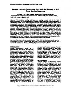
Figure 2: Variation of the kappa coefficient by increasing the number of input features.

Multilayer Perceptron) with different model parameters was conducted to assess how the discrimination of vegetation physiognomic classes varies with classifiers, input features, and ground truth data size. The cross-validation method showed that the Random Forests provided highest overall accuracy (0.81) and kappa coefficient (0.78). However, accuracy metrics did not vary much with experiments. Optimum number of features, the set of lowest number of input features yielding highest kappa coefficient, were large (more than 92) in all experiments. The large number of optimum features required by the experiments implied that multitemporal satellite data are crucial for discriminating the vegetation physiognomic types. Kappa coefficients were not highest by merely using all input features. Therefore, combination of the important features was found to be crucial for achieving the highest accuracy rather than just using the large number of input features. Generally, the kappa coefficient increased in all experiments by increasing the size of ground truth data sets. Still, discrimination of some classes especially between the coniferous and broadleaved forests was not adequate which requires further exploration in future.

Conflicts of Interest The authors declare that they have no conflicts of interest.

Kappa coefficients

0.8

Acknowledgments

0.7 0.6 0.5 0.4 0.3

25

50

75

100 125 150 175 200 225 250 275 300 Ground truth data size



Figure 3: Variation of the kappa coefficient by increasing the ground truth data size.

Fernández-Delgado et al. 2014 [51] found Random Forests as the better classifier than Support Vector Machines or Neural Networks after rigorous comparison of 179 classifiers (machine learning algorithms) using 121 different data sets.

4. Conclusions A set of machine learning experiments comprised of a number of supervised classifiers (𝑘-Nearest Neighbors, Gaussian Naive Bayes, Random Forests, Support Vector Machines, and

This research was partly supported by the Environment Research and Technology Development Fund (1-1405) of the Ministry of Environment, Japan, and Ministry of Education, Culture, Sports, Science and Technology (MEXT), Japan, Grant-in-Aid for Scientific Research (nos. 26350403 and P17F17109). The authors are grateful to the Biodiversity Center of Japan, Nature Conservation Bureau, Ministry of the Environment, for providing access to the vegetation survey data. The MOD09A1 and MYD09A1 products used in the research were available from the NASA EOSDIS Land Processes Distributed Active Archive Center (LP DAAC), USGS/Earth Resources Observation and Science (EROS) Center, Sioux Falls, South Dakota.

References [1] W. Köppen, Das geographische system der klimate, 1936. [2] A. W. Küchler, “A physiognomic classification of vegetation,” Annals of the Association of American Geographers, vol. 39, no. 3, pp. 201–210, 1949. [3] R. H. Whittaker, “Evolution and measurement of species diversity,” Taxon, vol. 21, pp. 213–251, 1972. [4] E. O. Box, “Predicting physiognomic vegetation types with climate variables,” Vegetatio, vol. 45, no. 2, pp. 127–139, 1981. [5] D. Grossman, D. Faber-Langendoen, A. Weakley et al., “International classification of ecological communities: terrestrial vegetation of the United States,” in Proceedings of The Nature Conservancy, Arlington, Va, USA, 1998. [6] R. H. Whittaker, “The Physiognomic Approach. In Classification of Plant Communities,” in Classification of Plant Communities, R. H. Whittaker, Ed., pp. 33–64, Springer, Dordrecht, Netherlands, 1978.

Scientifica [7] Z. Uchijima and H. Seino, “Probable effects of CO2 -induced climate change on natural vegetation of Japan,” Report of studies of evaluation of probable effects of CO, 1990. [8] H. Ohba, “The flora of Japan and the implication of global climatic change,” Journal of Plant Research, vol. 107, no. 1, pp. 85–89, 1994. [9] G. Leonelli, M. Pelfini, U. M. D. Cella, and V. Garavaglia, “Climate warming and the recent treeline shift in the european alps: The role of geomorphological factors in high-altitude sites,” Ambio, vol. 40, no. 3, pp. 264–273, 2011. [10] A. V. Kirdyanov, F. Hagedorn, A. A. Knorre et al., “20th century tree-line advance and vegetation changes along an altitudinal transect in the Putorana Mountains, northern Siberia,” Boreas, vol. 41, no. 1, pp. 56–67, 2012. [11] U. Büntgen, L. Hellmann, W. Tegel et al., “Temperature-induced recruitment pulses of Arctic dwarf shrub communities,” Journal of Ecology, vol. 103, no. 2, pp. 489–501, 2015. [12] A. Seim, K. Treydte, V. Trouet et al., “Climate sensitivity of Mediterranean pine growth reveals distinct east-west dipole,” International Journal of Climatology, vol. 35, no. 9, pp. 2503– 2513, 2015. [13] I. Gitas, C. Karydas, and G. Kazakis, “Land cover mapping of Mediterranean landscapes, using SPOT4-Xi and IKONOS imagery-A preliminary investigation,” in Options Mediterraneennes, pp. 27–41, Series B, 2003. [14] K. J. Salovaara, S. Thessler, R. N. Malik, and H. Tuomisto, “Classification of Amazonian primary rain forest vegetation using Landsat ETM+ satellite imagery,” Remote Sensing of Environment, vol. 97, no. 1, pp. 39–51, 2005. [15] L. Li, S. L. Ustin, and M. Lay, “Application of multiple endmember spectral mixture analysis (MESMA) to AVIRIS imagery for coastal salt marsh mapping: A case study in China Camp, CA, USA,” International Journal of Remote Sensing, vol. 26, no. 23, pp. 5193–5207, 2005. [16] P. H. Rosso, S. L. Ustin, and A. Hastings, “Mapping marshland vegetation of San Francisco Bay, California, using hyperspectral data,” International Journal of Remote Sensing, vol. 26, no. 23, pp. 5169–5191, 2005. [17] E. H. Helmer, T. S. Ruzycki, J. Benner et al., “Detailed maps of tropical forest types are within reach: Forest tree communities for Trinidad and Tobago mapped with multiseason Landsat and multiseason fine-resolution imagery,” Forest Ecology and Management, vol. 279, pp. 147–166, 2012. [18] C. L. Zweig, M. A. Burgess, H. F. Percival, and W. M. Kitchens, “Use of Unmanned Aircraft Systems to Delineate Fine-Scale Wetland Vegetation Communities,” Wetlands, vol. 35, no. 2, pp. 303–309, 2015. [19] Y. Su, Q. Guo, D. L. Fry et al., “A Vegetation Mapping Strategy for Conifer Forests by Combining Airborne LiDAR Data and Aerial Imagery,” Canadian Journal of Remote Sensing, vol. 42, no. 1, pp. 1–15, 2016. [20] T. T. Sankey, J. McVay, T. L. Swetnam et al., “UAV hyperspectral and lidar data and their fusion for arid and semi-arid land vegetation monitoring,” Remote Sensing in Ecology and Conservation, 2017. [21] M. Koch, T. Schmid, M. Reyes, and J. Gumuzzio, “Evaluating full polarimetric C- and L-band data for mapping wetland conditions in a semi-arid environment in central Spain,” IEEE Journal of Selected Topics in Applied Earth Observations and Remote Sensing, vol. 5, no. 3, pp. 1033–1044, 2012. [22] J. Betbeder, S. Rapinel, T. Corpetti, E. Pottier, S. Corgne, and L. Hubert-Moy, “Multitemporal classification of TerraSAR-X

7

[23]

[24]

[25]

[26]

[27]

[28]

[29]

[30]

[31]

[32]

[33]

[34]

[35]

[36]

[37]

data for wetland vegetation mapping,” Journal of Applied Remote Sensing, vol. 8, no. 1, Article ID 083648, 2014. H. Balzter, B. Cole, C. Thiel, and C. Schmullius, “Mapping CORINE land cover from Sentinel-1A SAR and SRTM digital elevation model data using random forests,” Remote Sensing, vol. 7, no. 11, pp. 14876–14898, 2015. L. F. D. A. Furtado, T. S. F. Silva, and E. M. L. D. M. Novo, “Dual-season and full-polarimetric C band SAR assessment for vegetation mapping in the Amazon várzea wetlands,” Remote Sensing of Environment, vol. 174, pp. 212–222, 2016. D. A. Roberts, M. E. Gardner, R. Church, S. L. Ustin, and R. O. Green, “Optimum strategies for mapping vegetation using multiple-endmember spectral mixture models,” in Proceedings of Imaging Spectrometry III, pp. 108–119, usa, July 1997. M. Chikr El-Mezouar, N. Taleb, K. Kpalma, and J. Ronsin, “An IHS-based fusion for color distortion reduction and vegetation enhancement in IKONOS imagery,” IEEE Transactions on Geoscience and Remote Sensing, vol. 49, no. 5, pp. 1590–1602, 2011. T. Udelhoven, “Long term data fusion for a dense time series analysis with MODIS and Landsat imagery in an Australian Savanna,” Journal of Applied Remote Sensing, vol. 6, no. 1, p. 63512, 2012. M. Schmidt, R. Lucas, P. Bunting, J. Verbesselt, and J. Armston, “Multi-resolution time series imagery for forest disturbance and regrowth monitoring in Queensland, Australia,” Remote Sensing of Environment, vol. 158, pp. 156–168, 2015. H. Murray, A. Lucieer, and R. Williams, “Texture-based classification of sub-Antarctic vegetation communities on Heard Island,” International Journal of Applied Earth Observation and Geoinformation, vol. 12, no. 3, pp. 138–149, 2010. N. Stuart, T. Barratt, and C. Place, “Classifying the neotropical savannas of Belize using remote sensing and ground survey,” Journal of Biogeography, vol. 33, no. 3, pp. 476–490, 2006. Z.-W. Wang, Q. Wang, L. Zhao et al., “Mapping the vegetation distribution of the permafrost zone on the Qinghai-Tibet Plateau,” Journal of Mountain Science, vol. 13, no. 6, pp. 1035– 1046, 2016. M. Schwieder, P. J. Leitão, M. M. da Cunha Bustamante, L. G. Ferreira, A. Rabe, and P. Hostert, “Mapping Brazilian savanna vegetation gradients with Landsat time series,” International Journal of Applied Earth Observation and Geoinformation, vol. 52, pp. 361–370, 2016. A. M. Filippi and J. R. Jensen, “Fuzzy learning vector quantization for hyperspectral coastal vegetation classification,” Remote Sensing of Environment, vol. 100, no. 4, pp. 512–530, 2006. K. A. Vanselow and C. Samimi, “Predictive mapping of dwarf shrub vegetation in an arid high mountain ecosystem using remote sensing and random forests,” Remote Sensing, vol. 6, no. 7, pp. 6709–6726, 2014. N. Torbick, L. Ledoux, W. Salas, and M. Zhao, “Regional mapping of plantation extent using multisensor imagery,” Remote Sensing, vol. 8, no. 3, article no. 236, 2016. G. A. Carpenter, S. Gopal, S. MacOmber, S. Martens, and C. E. Woodcock, “A neural network method for mixture estimation for vegetation mapping,” Remote Sensing of Environment, vol. 70, no. 2, pp. 138–152, 1999. C. Zhang and Z. Xie, “Combining object-based texture measures with a neural network for vegetation mapping in the Everglades from hyperspectral imagery,” Remote Sensing of Environment, vol. 124, pp. 310–320, 2012.

8 [38] O. Antropov, Y. Rauste, H. Astola, J. Praks, T. Hame, and M. T. Hallikainen, “Land cover and soil type mapping from spaceborne polsar data at l-band with probabilistic neural network,” IEEE Transactions on Geoscience and Remote Sensing, vol. 52, no. 9, pp. 5256–5270, 2014. [39] R. C. Sharma, K. Hara, H. Hirayama et al., “Production of MultiFeatures Driven Nationwide Vegetation Physiognomic Map and Comparison to MODIS Land Cover Type Product,” Advances in Remote Sensing, vol. 06, no. 01, pp. 54–65, 2017. [40] C. J. Tucker, “Red and photographic infrared linear combinations for monitoring vegetation,” Remote Sensing of Environment, vol. 8, no. 2, pp. 127–150, 1979. [41] A. Huete, K. Didan, T. Miura, E. P. Rodriguez, X. Gao, and L. G. Ferreira, “Overview of the radiometric and biophysical performance of the MODIS vegetation indices,” Remote Sensing of Environment, vol. 83, no. 1-2, pp. 195–213, 2002. [42] X. Xiao, S. Boles, S. Frolking et al., “Landscape-scale characterization of cropland in China using Vegetation and Landsat TM images,” International Journal of Remote Sensing, vol. 23, no. 18, pp. 3579–3594, 2002. [43] J. Cohen, “A coefficient of agreement for nominal scales,” Educational and Psychological Measurement, vol. 20, no. 1, pp. 37–46, 1960. [44] R. C. Sharma, R. Tateishi, K. Hara, and K. Iizuka, “Production of the Japan 30-m land cover map of 2013—2015 using a random forests-based feature optimization approach,” Remote Sensing, vol. 8, no. 5, article no. 429, 2016. [45] Y. Y. Wang and J. Li, “Feature-selection ability of the decisiontree algorithm and the impact of feature-selection/extraction on decision-tree results based on hyperspectral data,” International Journal of Remote Sensing, vol. 29, no. 10, pp. 2993–3010, 2008. [46] M. Pal and G. M. Foody, “Feature selection for classification of hyperspectral data by SVM,” IEEE Transactions on Geoscience and Remote Sensing, vol. 48, no. 5, pp. 2297–2307, 2010. [47] B. Waske, S. van der Linden, J. A. Benediktsson, A. Rabe, and P. Hostert, “Sensitivity of support vector machines to random feature selection in classification of hyperspectral data,” IEEE Transactions on Geoscience and Remote Sensing, vol. 48, no. 7, pp. 2880–2889, 2010. [48] F. Löw, U. Michel, S. Dech, and C. Conrad, “Impact of feature selection on the accuracy and spatial uncertainty of per-field crop classification using Support Vector Machines,” ISPRS Journal of Photogrammetry and Remote Sensing, vol. 85, pp. 102– 119, 2013. [49] G. M. Foody and A. Mathur, “Toward intelligent training of supervised image classifications: directing training data acquisition for SVM classification,” Remote Sensing of Environment, vol. 93, no. 1-2, pp. 107–117, 2004. [50] Z. Zhu, A. L. Gallant, C. E. Woodcock et al., “Optimizing selection of training and auxiliary data for operational land cover classification for the LCMAP initiative,” ISPRS Journal of Photogrammetry and Remote Sensing, vol. 122, pp. 206–221, 2016. [51] M. Fernández-Delgado, E. Cernadas, S. Barro, and D. Amorim, “Do we need hundreds of classifiers to solve real world classification problems,” Journal of Machine Learning Research, vol. 15, pp. 3133–3181, 2014.

Scientifica

Journal of

Journal of

Waste Management

Hindawi Publishing Corporation http://www.hindawi.com

The Scientific World Journal Volume 2014

International Journal of

Ecology

Environmental and Public Health


Volume 2014

Scientifica Hindawi Publishing Corporation http://www.hindawi.com

Volume 2014


Volume 2014


Volume 2014

Journal of

Ecosystems


Oceanography Hindawi Publishing Corporation http://www.hindawi.com


Volume 2014

Volume 2014

Submit your manuscripts at https://www.hindawi.com Journal of


Marine Biology

Atmospheric Sciences Hindawi Publishing Corporation http://www.hindawi.com


Journal of

Biodiversity Hindawi Publishing Corporation http://www.hindawi.com

Geological Research Volume 2014


Volume 2014

Journal of Computational Environmental Sciences

Journal of

Earthquakes Hindawi Publishing Corporation http://www.hindawi.com


Volume 2014

Volume 2014


Volume 2014


Forestry Research Hindawi Publishing Corporation http://www.hindawi.com

Volume 2014

*HRSK\VLFV International Journal of


Volume 201

$SSOLHG (QYLURQPHQWDO 6RLO6FLHQFH +LQGDZL3XEOLVKLQJ&RUSRUDWLRQ KWWSZZZKLQGDZLFRP

Journal of

Climatology 9ROXPH


Volume 2014

Advances in

Environmental Chemistry

Advances in

Meteorology Hindawi Publishing Corporation http://www.hindawi.com

Volume 2014

Volume 2014


Volume 2014