A Machine Learning Approach to Anomaly Detection Philip K. Chan, Matthew V. Mahoney, and Muhammad H. Arshad Department of Computer Sciences Florida Institute of Technology Melbourne, FL 32901 pkc, mmahoney,
[email protected] March 29, 2003 Technical Report CS-2003-06 Abstract Much of the intrusion detection research focuses on signature (misuse) detection, where models are built to recognize known attacks. However, signature detection, by its nature, cannot detect novel attacks. Anomaly detection focuses on modeling the normal behavior and identifying significant deviations, which could be novel attacks. In this paper we explore two machine learning methods that can construct anomaly detection models from past behavior. The first method is a rule learning algorithm that characterizes normal behavior in the absence of labeled attack data. The second method uses a clustering algorithm to identify outliers.
Keywords: anomaly detection, machine learning, intrusion detection
1
Introduction
The Internet is one of the most influential innovations in recent history. Though most people use the Internet for productive purposes, some use it as a vehicle for malicious intent. As the Internet links more users together and computers are more prevalent in our daily lives, the Internet and the computers connected to it increasingly become more enticing targets of attacks. Computer security often focuses on preventing attacks using usually authentication, filtering, and encryption techniques, but another important facet is detecting attacks once the preventive measures are breached. Consider a bank vault, thick steel doors prevent intrusions, while motion and heat sensors detect intrusions. Prevention and detection complement each other to provide a more secure environment. How do we know if an attack has occurred or has been attempted? This requires analyzing huge volumes of data gathered from the network, host, or file systems to find suspicious activity. Two general approaches exist for this problem: signature detection (also known as misuse detection), where we look for patterns signaling well-known attacks, and anomaly detection, where we look for deviations from normal behavior. Signature detection works reliably on known attacks, but has the obvious disadvantage of not capable of detecting new attacks. Though anomaly detection can detect novel attacks, it has the drawback of not capable of discerning intent; it can only signal that some event is unusual, but not necessarily hostile, thus generating false alarms. A desirable system would employ both approaches. Signature detection methods are more well understood and widely applied. They are used in both host based systems, such as virus detectors, and in network based systems such as SNORT [32] and BRO [26]. These systems use a set of rules encoding knowledge gleaned from security experts to test files or network traffic for patterns known to occur in attacks. As new vulnerabilities or attacks are discovered, the rule set must be manually updated, a limitation of such systems. Also minor variations in attack methods can often defeat such systems. For anomaly detection, a model of acceptable behavior can also be specified by humans as well. For example, firewalls are essentially manually written policies dictating what network traffic is considered normal and acceptable. 1
How do security experts discover new unknown attacks? Generally, the experts identify something out of ordinary, which triggers further investigation. Some of these investigations result in discovering new attacks, while others result in false alarms. From their experience, security experts have learned a model of normalcy and use the model to detect abnormal events. We desire to endow computers with the capability of identifying unusual events similar to humans by learning (data mining) from experience, i.e., historical data. Since what is considered normal could be different in different environments, a distinct model of normalcy need to be learned individually. This contrasts to manually written polices of normal behavior that require manual customization at each environment. Moreover, since the models are customized to each environment, potential attackers would find them more difficult to circumvent than manually written policies that might be less customized due to inexperienced system administrators who do not change the default parameters and policies supplied by the vendors. Our goal is to learn anomaly detectors that can be customized to individual environments. This goal has a few challenges. First, anomaly detection is a harder problem than signature detection because signatures of attacks can be very precise but what is considered normal is more abstract and ambiguous. Second, classical machine learning problems are classification tasks—given examples of different classes, learn a model that distinguishes the different classes. However, in anomaly detection, we are essentially given only one class of examples (normal instances) and we need to learn a model that characterizes and predicts the lone class reliably. Since examples of the other classes are absent, traditional machine learning algorithms are less applicable to anomaly detection. Thrid, research in anomaly detection uses the approach of modeling normal behavior from a (presumably) attack-free training set. However, clean data for training may not be easy to obtain. Lastly, to help humans analyze the alerts, anomaly detectors need to be able to describe the anomalies, though not as precise as signature detectors are capable. To meet the second challenge, we propose two methods for learning anomaly detectors: rule learning (LERAD) and clustering (CLAD). CLAD does not assume the training data are free of attacks—the third challenge. For the last challenge, our models are not black boxes and alerts can be explained by rules that are violated in LERAD or by the centroids of the “near miss” normal clusters in CLAD. Our experimental results indicate that, though anomaly detection is a harder problem (the first challenge), our methods can detect attacks with relatively few false alarms. This article is organized as follows. Section 2 contrasts related techniques in anomaly detection. Section 3 proposes the LERAD algorithm that learns the characterization of normal behavior in logical rules. Section 4 describes a clustering algorithm that can identify behavior far from the normal behavior. We summarize our findings and suggest improvements in Section 5.
2
Related Work
Anomaly detection is related to biological immunology. Forrest et al. [12] observe that part of our immune system functions by identifying unfamiliar foreign objects and attacking them. For example, a transplanted organ is often attacked by the patient’s immune system because the organ from the donor contains objects different from the ones in the patient. Forrest et al. found that when a vulnerable UNIX system program or server is attacked (for example, using a buffer overflow to open a root shell), that the program makes sequences of system calls that differ from the sequences found in normal operation [13]. Forrest used ngram models (sequences of n = 3 to 6 calls), and matching them to sequences observed in training. A score is generated when a sequence observed during detection is different from those stored during training. Other models of normal system call sequences have been used, such as finite state automata [34] and neural networks [14]. Notably, Sekar et al. [34] utilize program counter information to specify states. Though the program counter carries limited information about the state of a program, its addition to their model is different from typical n-gram models that solely rely on sequences of system calls. Lane and Brodley [19] use instance-based methods and Sequeira and Zaki [35] use clustering methods for detecting anomalous user commands. A host-based anomaly detector is important since some attacks (for example, inside attacks) do not generate network traffic. However, network-based anomaly detector can warn attacks launched from the outside at an earlier stage, before the attacks actually reach the host, than host-based anomaly detectors.
2
Current network anomaly detection systems such as NIDES [3], ADAM [5], and SPADE [8] model only features of the network and transport layer, such as port numbers, IP addresses, and TCP flags. Models built with these features could detect probes (such as port scans) and some denial of service (DOS) attacks on the TCP/IP stack, but would not detect attacks of the type detected by Forrest, where the exploit code is transmitted to a public server in the application payload. Network anomaly detectors estimate the probabilities of events, such as that of a packet being addressed to some port, based on the frequency of similar events seen during training or during recent history, typically several days. They output an anomaly score which is inversely proportional to probability. Anomaly detectors are typically just one component of more comprehensive systems. NIDES is a host-based anomaly detection component of EMERALD [24], which integrates the results from host and network-based detectors. ADAM is a Bayes classifier with categories for normal behavior, known attacks, and unknown attacks. SPADE is a SNORT [32] plug-in. Some anomaly detection algorithms are for specific attacks (e.g., portscans [36]) or services (e.g., DNS [18]). Most current anomaly detectors use a stationary model, where the probability of an event depends on its average rate during training, and does not vary with time. However, using the average rate could be incorrect for many processes. Paxon and Floyd [27] found that many network processes, such as the rate of a particular type of packet, have self-similar (fractal) behavior. Events do not occur at uniform rates on any time scale. Instead they tend to occur in bursts. Hence, it is not possible to predict the average rate of an event over a time window by measuring the rate in another window, regardless of how short or long the windows are. An example of how a stationary model fails in an anomaly detector would be any attack with a large number of events, such as a port scan or a flooding attack. Clustering and related techniques have been used to locate outliers in a dataset. Knorr and Ng [17] define an outlier as an object with at least p fraction of the dataset is farther than distance D from the object, where p and D are parameters specified by the users. Instead of a global perspective [17], LOF [6] uses a local perspective and locates outliers with respect to the density in the local/neighboring region. They illustrate the inability of conventional approaches to detect such outliers. LOF has two short-comings: one, their approach is very sensitive to the choice of M inP ts, which specifies the minimum number of objects allowed in the local neighborhood (similar to k in k-NN, k-Nearest Neighbor); second, and more importantly, their approach is not well-suited for very high dimensional data such as network traffic data. Ramaswamy et al. [31] investigate the problem of finding the top n outliers. They characterize an outlier by the distance of the kth-nearest neighbor and their algorithm efficiently partitions the input space and prunes partitions that cannot contain the top outliers. Aggarwal and Yu [1] calculate the sparsity coefficient, which compares the observed and expected number of data points, in “cubes” (spatial grid cells) generated by projections on the dataset.
3
Learning Rules for Anomaly Detection (LERAD)
To build a model for anomaly detection, from a probabilistic perspective, one can attempt to estimate P (x|DN oAttacks ), where x is an instance under consideration and DN oAttacks is a data set of instances that do not contain attacks. Since all the probabilistic estimations are based on the training data set D N oAttacks , for notation convenience, we use P (x) in lieu of P (x|DN oAttacks ). Under this model, the smaller P (x) is, the more likely x is anomalous. Each instance x is represented by values from a set of m attributes a1 , a2 , ..., am . That is, x is a tuple of values (a1 = v1 , a2 = v2 , ..., am = vm ), where vi is the value for attribute ai . The probability P (x) is hence: P (a1 = vi , a2 = v2 , ..., am = vm ) or more concisely, P (vi , v2 , ..., vm ). Using the chain rule is frequently is too computationally expensive. Some researchers assume the attributes to be independent in “Naive” Bayes algorithms [10, 7, 9]. However this assumption is usually invalid. To incorporate attribute dependence, Bayesian networks [28] model a subset of the conditional probabilities structured in networks, which are selected using prior knowledge. Recent work in Bayesian networks attempts to learn the network structures from data. However, Bayesian networks model the entire distribution of each conditional probability and could consume significant computational resources. Instead of estimating the probability of an instance x, an alternative approach is to estimate the likelihood of values among the attributes in each instance. That is, given some attribute values, we estimate the likeli-
3
hood of some other attribute values. Again, consider v1 , ..., vm = V are the values of attributes a1 , ..., am of an instance. Let U ⊂ V , W ⊂ V , and U ∩ W = ∅, we would like to estimate: P (W |U ). For example, consider these network packet values: V = {SrcIp = 128.1.2.3, DestIp = 128.4.5.6, SrcP ort = 2222, DestP ort = 80}. Further we consider U = {SrcIp = 128.1.2.3, DestIp = 128.4.5.6} and W = {DestP ort = 80}, hence P (W |U ) is: P (DestP ort = 80|SrcIp = 128.1.2.3, DestIp = 128.4.5.6). In anomaly detection we seek combinations of U and W with large P (W |U )—W is highly predictive by U . These combinations indicate patterns in the normal training data and fundamentally constitute a model that describes normal behavior. If these patterns are violated during detection, we calculate a score that reflects the severity of the violation and hence the degree of anomaly. That is, the anomaly score depends on P (¬W |U ), where W , though expected, is not observed when U is observed. Finding these patterns could be computationally expensive since the space of combinations is O(d m ), where d is the domain size of an attribute and m is the number of attributes. In the next section we describe our proposed learning algorithm.
3.1
LERAD Algorithm
Our goal is to design an efficient algorithm that finds combinations of U and W with large P (W |U ) during training and uses P (¬W |U ) to calculate an anomaly score during detection. The task of finding combinations of U and W is similar to finding frequent patterns in association rules [2], where U is the antecedent, W is the consequent, and P (W |U ) is the confidence. Algorithms for finding association rules, for example Apriori [2], typically find all rules that exceed the user-supplied confidence and support thresholds; consequently, a large number of rules can be generated. Checking large number of rules during detection incurs unacceptable amounts of overhead. However, our goal is different from finding association rules in two fundamental respects. First, the semantics of our rules are designed to estimate P (¬W |U ). Second, we want a “minimal” set of rules that succinctly describes the normal training data. These differences are exhibited in our proposed rules and algorithm called LERAD (LEarning Rules for Anomaly Detection). 3.1.1
Semantics of LERAD Rules
The semantics of LERAD rules seek to estimate P (¬W |U ); in rule form, a LERAD rule is: U ⇒ ¬W
[p = P (¬W |U )],
(1)
where p denotes P (¬W |U ) and reflects the likelihood of an anomaly. These rules can be considered as anomaly rules. We also extend the semantics of W . In the consequent instead of allowing a single value for each attribute, our rules allow each attribute to be an element of a set of values. For example, consider W = {DestP ort ∈ {21, 25, 80}} (instead of W = {DestP ort = 80}), P (W |U ) is: P (DestP ort ∈ {21, 25, 80}|SrcIp = 128.1.2.3, DestIp = 128.4.5.6) and P (¬W |U ) becomes: P (DestP ort 6∈ {21, 25, 80}|SrcIp = 128.1.2.3, DestIp = 128.4.5.6) or in rule form: SrcIp = 128.1.2.3, DestIp = 128.4.5.6 ⇒ DestP ort 6∈ {21, 25, 80} [p]. Given U , the set of values for each attribute in W represents all the values seen in the training data for that particular attribute. Following the above example, given SrcIp = 128.1.2.3 and DestIp = 128.4.5.6, DestP ort is either 21, 25, or 80 in the normal training data. This extension allows our models to be more predictive and conservative so that false alarms are less likely to occur. However, since W includes all the seen values in training, a simplistic estimation of P (W |U ) would yield 1 and P (¬W |U ) 0. Obviously, these estimates are too extreme. Since event ¬W is not observed when event U is observed during training, estimating P (¬W |U ) becomes a “zero-frequency” problem [37]. 3.1.2
Zero-frequency Problem
Laplace smoothing is commonly used in the machine learning community to handle the zero-frequency problem [25, 23, 30]. One variant of the technique is to assign a frequency of one, instead of zero, to each event at the beginning. Hence, all events, observed or not, will have at least a count of one and none of the events have an estimated probability of zero. That is, assuming the total number of unique 1 , where events is unknown, the likelihood of a novel event can be estimated by: P (N ovelEvent) = n+r+1 n is the total number of observed events and r is the number of unique observed events. The one in the numerator and denominator is for the unobserved event. For example, consider a sequence of ten events:
4
Table 1: Example Training Data Set D = {di } for i = 1..6 (marked by rk in Step 3) di d1 d2 d3 d4 d5 d6
a1 1 1 2 2 1 2
a2 2 (r2 ) 2 (r2 ) 6 (r1 ) 7 2 8
a3 3 3 3 3 3 3
a4 4 5 5 5 4 4
in subset DS and DT DS and DT DS and DT DT DV DV
S1 = 1, 2, 3, 4, 5, 6, 2, 7, 4, 8; P (N ovelEvent) = P (x 6∈ {1, 2, 3, 4, 5, 6, 7, 8}) = 1/(10 + 8 + 1) = 1/19. For another sequence: S2 = 1, 1, 1, 1, 1, 1, 1, 1, 1, 1; P (N ovelEvent) = P (x 6∈ 1) = 1/(10 + 1 + 1) = 1/12. However, in terms of relative ranking of P (N ovelEvent) for S1 and S2 , the above Laplace estimates are counter intuitive. The events in S2 are homogeneous, always 1, however, the events in S1 are quite diverse. Intuitively, the likelihood of seeing something novel in S1 should be larger than S2 , but the estimates indicate otherwise. Witten and Bell [37] proposed a few estimates for novel events in the context of data compression; one estimate is: r P (N ovelEvent) = . (2) n This measures the average rate of novel values in the sample. Using our two examples above, P (N ovelEvent) = 8/10 for S1 and P (N ovelEvent) = 1/10 for S2 . Their relative ranking conforms to our intuition. (Our examples grossly over estimate the likelihood because n is small, but n is usually in the millions in our tasks.) Eq. 2 is used to estimate p = P (¬W |U ) in Eq. 1, where n is the number of instances satisfying the antecedent U and r is the number of unique values in the attribute of the consequent W . We attempted more sophisticated estimators in initial experiments for anomaly detection, but Eq. 2 seems to perform as effectively as others and requires the least computation, which is advantageous in mining large amounts of data. 3.1.3
Randomized Algorithm
In the previous sections we have discussed the semantics of LERAD rules and how P (¬W |U ) can be estimated. We now discuss an efficient algorithm that finds combinations of U and W with low P (¬W |U ) (or high P (W |U )). Our algorithm is based on sampling and randomization. Let D be the entire training data set, DT and DV be the training and validation sets respectively such that DT ∪ DV = D, DT ∩ DV = ∅, and |DT | > |DV |, and DS is a random sample of DT such that DS ⊂ DT and |DS | ¿ |DT |. DE is a separate test/evaluation set disjoint from the training set D. Our proposed mining algorithm consists of five main steps: 1. 2. 3. 4. 5.
generate candidate rules from DS , evaluate candidate rules from DS , select a “minimal” set of candidate rules that covers DS , train the selected candidate rules on DT , and prune the rules that cause false alarms on DV
Steps 1-3 intend to select a small and predictive set of rules from a small sample D S of the data. The selected rules are then trained on the much larger set DT in Step 4. The validation set DV is used to reduce overfitting in Step 5. For simplicity, we only consider rules that have only one attribute in the consequent. Further details are in [21]. Step 1: Pairs of instances are randomly chosen from DS . For each pair of instances, we identify the matching attribute values between the two instances. Consider d1 and d2 in Table 1 as a random pair, a1 = 1, a2 = 2, and a3 = 3 occur in both instances. The three values are then chosen in random order, e.g., a2 = 2, a1 = 1, and a3 = 3; and the candidate rules in Table 2 are generated. The first value (a2 = 2) is chosen to be in the consequent (W ) and the the later values are iteratively added to the antecedent (U ). In
5
Table 2: Rules (rk ) Generated by LERAD Steps 1-5 Step 1 r 1 : ∗ ⇒ a2 = 2 r2 : a1 = 1 ⇒ a 2 = 2 r2 : a1 = 1, a3 = 3 ⇒ a2 = 2 Step 3 r2 : a1 = 1 ⇒ a2 6∈ {2}[p = 1/2] r1 : ∗ ⇒ a2 6∈ {2, 6}[p = 2/3]
Step 2 r1 : ∗ ⇒ a2 ∈ {2, 6} r 2 : a1 = 1 ⇒ a 2 = 2 r3 : a1 = 1, a3 = 3 ⇒ a2 = 2 Step 4 r2 : a1 = 1 ⇒ a2 6∈ {2}[p = 1/2] r1 : ∗ ⇒ a2 6∈ {2, 6, 7}[p = 3/4]
Step 2 (rewritten in Eq.1 form) r1 : ∗ ⇒ a2 6∈ {2, 6}[p = 2/3] r2 : a1 = 1 ⇒ a2 6∈ {2}[p = 1/2] r3 : a1 = 1, a3 = 3 ⇒ a2 6∈ {2}[p = 1/2] Step 5 r2 : a1 = 1 ⇒ a2 6∈ {2}[p = 1/3]
r1 ∗ is a wild card and matches anything. If the matching attribute values occur often in different instances, they will likely be found matching again in another randomly chosen pair of instances and more rules for these matching attribute values will be generated. That is, the more likely the values are correlated, more rules will be generated to describe the correlation (duplicate rules are removed). Step 2: We evaluate the candidate rules on DS . Note that the consequent in the candidate rules generated from Step 1 has only one value. In Step 2 we add values to the attribute in the consequent if more values are observed in DS . d1 and d2 do not change the rules. d3 causes r1 is to be updated because a2 = 6 in d3 ; the other two rules are unchanged because the antecedents are not satisfied for d 3 . The new set of candidate rules are in Table 2. We then write the rules in the form of Eq. 1 and estimate p = P (¬W |U ) for each rule by using Eq. 2 in Table 2. Step 3: We select a “minimal” subset of candidate rules that sufficiently describe D S . Our method is based on two heuristics. First, we prefer rules with lower p = P (¬W |U ). Second, a rule can cover multiple instances in DS , but an instance does not need to be covered by more than one rule (more details later). Hence, we sort the rules based on p and evaluate the rules in ascending order. For each rule, we mark instances that are covered by the rule. If a rule cannot mark any remaining unmarked instances, it is removed. That is, we keep rules with lower p and remove rules that do not contribute to covering instances not covered by previous rules with lower p values. Step 4: This step is similar to Step 2, except that the rules are updated based on D T , instead of DS . d4 does not affect r2 since its antecedent does not match. However, 7 is added to the consequent of r 1 and p is updated to 3/4 in Table 2. After Step 4, the rules have been trained from DT . Step 5: Since all instances in the validation set DV are normal, an alarm generated by a rule with any instance in DV is a false alarm. To reduce overfitting, during Step 5, we remove rules that generate alarms in the validation set. Using our running example, d5 is normal according to r1 and r2 . However, r1 generates an alarm for d6 since a2 = 8 6∈ {2, 6, 7}. r2 does not generate an alarm because a1 = 2, which does not satisfy the antecedent of r2 . Hence, only r2 remains in Table 2. During Step 5, to fully utilize legitimate training data in the validation set, we also update p for rules that are not removed. Hence, p for r 2 was updated to 1/3. 3.1.4
Anomaly Score and Nonstationary Model
During training, a set of anomaly rules R that “minimally” describes the training data are generated and their p = P (¬W |U ) is estimated. During detection, given an instance x, we generate an anomaly score if x satisfies any of the anomaly rules (U ⇒ ¬W ). Let SP ⊂ R be the set of anomaly rules that x satisfies. The anomaly score is calculated as: AnomalyScore(x) = rk ∈S p1k , where rk is a rule in S and pk is the p value of rule rk . The reciprocal of pk reflects a surprise factor that is large when anomaly has a low likelihood (small pk ). The p estimate is an aggregate over a stationary training period; however, recent events can greatly influence current events. Bursty network traffic or OS activities are common. In intrusion detection we experience that attacks cause bursty behavior as well. In order to incorporate recent novel events into our
6
scoring mechanism, we introduce tk which is the duration since the last novel value was observed in the consequent of anomaly rule rk (or when rk was satisfied). The smaller tk is, the higher the likelihood that we will see another novel value. That is, intuitively, we are less surprised if we have observed a novel value in a more recent past. Hence, we calculate the anomaly score as: AnomalyScore(x) =
X tk . pk
(3)
rk ∈S
3.2
Summary of Current Results
To evaluate LERAD, we use network traffic recorded in tcpdump provided by the DARPA evaluation in 1999 [20, 16]. Week 3 was used for training (D) and Weeks 4 and 5 (DE ) were used for testing. The size of the validation set (|DV |) was set to be 10% of the training set (D). LERAD was run five times with a different random seed. Attributes used in our data sets include values in the protocol header and application payload. LERAD is evaluated based on the number of detected attacks with at most 10 false alarms per day. In our experiments the resulting set of rules usually contains 50 to 75 rules. Though the rule set is relatively small, LERAD, on the average, detects about 117 attacks out of 201 attacks with at most 10 false alarms per day. Under a “blind” evaluation (the test set was not available apriori), the original DARPA participant with the most detections detected 85 attacks [20]. This indicates LERAD is quite successful in finding highly predictive normal patterns. More importantly, LERAD detects about 58% of the attacks poorly detected by the original participants [20]. That is, LERAD increases the overall coverage of detectable attacks. The total computational overhead is about 30 minutes for three weeks of training and test data. Much of the overhead is in preprocessing of the raw data to generate feature values for training and testing. Training and testing on three weeks of data take less than two minutes. We also analyzed and categorized why our detected anomalies were successful in detecting attacks. The more common categories (covering about 70% of the detected attacks) are unexpected user behavior (e.g., unusual client addresses for servers) and learned (partial) attack signatures (e.g., unusual input that exploit bugs in software). Details of our findings are described in [21]. Furthermore, details of our results of our earlier and simplier algorithms PHAD and ALAD are in [22]. Our PHAD algorithm was adapted to detect attacks by modeling accesses to the Registry in the Windows OS [4].
4
Clustering for Anomaly Detection (CLAD)
LEARD assumes the training data are free of attacks, however, making sure the data is clean could be time consuming. We propose to use a clustering approach to identify “outliers” as anomalous. Our clustering method, CLAD, is inspired by the work of [11, 29], and is related to k-NN. CLAD locates anomalies by finding local and global outliers with some restrictions, where k-NN and LOF [6] concentrate mainly on local outliers. One key difference of CLAD from other clustering algorithms is that clusters are of fixed width (radius) and allows clusters to overlap (i.e., the clusters are not mutually exclusive). This difference permits CLAD to process large amounts of data efficiently. CLAD has two phases: Phase 1 creates the clusters and Phase 2 assigns data points to additional clusters. Fig. 1 illustrates the steps of the 2 phases. Given a dataset, D, Phase 1 creates clusters of fixed width, W (which will be discussed later), and assigns data points, d ∈ D, to the created clusters. If a data point is further away than width W from any existing cluster, the data point becomes the centroid of a new cluster; otherwise it is assigned to all existing clusters that are not further away than W . In Phase 1 since data points can only be assigned to existing clusters, some data points might miss assignment to clusters that are subsequently created. Phase 2 assigns these data points to additional clusters. So far our CLAD algorithm is basically the clustering algorithm proposed in [11, 29], however, the methods significantly diverge on how data points are represented for calculating distance, how the cluster width is determined, and how the properties of outliers are decided.
7
Input: Dataset D Output: Set of clusters C 1. initialize the set of clusters, C, to ∅ Phase 1: Creating clusters 2. for d ∈ D 3. for c ∈ C 4. if distance(d, c) ≤ W , assign d to c 5. if d is not assigned 6. create cluster c0 with d as the centroid and add c0 to C Phase 2: Assigning data points to additional clusters 7. for d ∈ D 8. for c ∈ C 9. if distance(d, c) ≤ W and d is not assigned to c 10. assign d to c Figure 1: Overall CLAD Algorithm
4.1
Feature Vectors and Distance Function
Each data point, d, is represented by a feature vector, and a cluster, c, is represented by its centroid, which is a data point. We use the Euclidean distance as our distance function: v u |Y1 | uX distance(Y1 , Y2 ) = t (Y1j − Y2j )2 , (4) j=1
where Y1 and Y2 are two feature vectors, Yij denotes the jth component of Yi , and |Yi | denotes the length of vector Yi . To obtain a feature vector for a data point, we transform the data points represented in the input attribute vectors (Xi ) into our feature vectors (Yi ). We have two types of transformation depending on whether the input attribute is continuous or discrete. Discrete attributes are usually problematic for distance functions. In anomaly detection since values that are observed more frequently are less likely to be anomalous and we want distance to indicate the difference in the degree of normalcy (separating normal from abnormal behavior), we represent a discrete value by its frequency. That is, discrete values of similar frequency are close to each other, but values of very different frequency are far apart. As a result, discrete attributes are transformed to continuous attributes. In our domain continuous attributes, including those transformed from discrete attributes, usually exhibit a power-law distribution—smaller values are much more frequent than larger values. Distances involving the infrequent large values are large and “drowns” the distances involving only small values. To reduce this problem, we use a logarithmic scale. In addition, to discount variance among values, we quantize the values using the floor operation, after taking the logarithm. Furthermore, in order to consider each attribute equally, the values of each attribute are normalized to the range [0,1]. Formally, an input attribute value, Xij , is transformed to a, feature value, Yij as follows: Yij = normalize(bln(Xij + 1)c),
(5)
where normalize(vj ) = (vj − M inj )/(M axj − M inj ), vj is a value from vector component j, and M inj (M axj ) is the minimum (maximum) value of component j. To avoid negative and undefined values (when 0 ≤ Xij < 1) , we add 1 to Xij before taking ln. For normalization, we also considered the number of standard deviations (SD) away from average. However, power-law distributions are one-sided and heavy-tailed, so standard deviations are not very appropriate for our purpose. Using SD for normalization resulted in noticeable degradation in performance in our experiments. Therefore, we revert to simple scaling as a means of normalization. 8
4.2
Cluster Width
The cluster width, W , specifies the local neighborhood of clusters that are considered close. The width is specified by the user in [29]. CLAD derives the width from the smallest distances between pairs of data points. To efficiently calculate the width, CLAD randomly draws a sample, of size s = 1% × |D|, from the entire dataset, D, and calculates the pair-wise distances. The bottom 1% of the pair-wise distances (i.e., 1% × s(s − 1)/2 pairs) are considered the smallest and their average is the cluster width. That is, CLAD samples pair-wise distances and uses the average distance of the closest neighbors as W . Though CLAD has a fixed parameter of 1% for deriving W , it is much less ad hoc than asking the user to specify W , which becomes a parameter. Our parameter is similar to specifying k in k-NN methods, but our parameter is in relative percentage, which is different from the absolute count of k and is conceptually easier to specify and understand.
4.3
Density, Inter-cluster Distance, and Anomalies
To determine if a cluster is an outlier, CLAD relies on two properties of a cluster: density and distance from the other clusters. Since each cluster has the same W (and hence “area”), we define the density of cluster ci as the number of data points, Counti , in ci . For the distance from the other clusters, we calculate the average inter-cluster distance (ICD) between ci and the other clusters. Formally, we denote ICDi as the ICD of cluster ci and define ICDi as: ICDi =
|C| X 1 distance(ci , cj ) |C| − 1
(6)
j=1,6=i
where C, as similarly defined before, is the set of clusters. Clusters that are distant and sparse are considered outliers and anomalous. A cluster c i is considered distant if ICDi is more than a standard deviation away from the average ICD. From our initial experiments, we observe that the distribution of Count exhibits a power-law distribution; when we use average and SD for Count, the average is very small and few/no clusters have Counti one SD smaller than the average. Hence, instead of using the average we use the median; a cluster ci is considered sparse when Counti is more than one median absolute deviation (MAD) [15] smaller than the median Count. Interestingly, in our domain an attack could be composed of many data points (e.g., flooding attacks), and hence dense regions could be attacks as well. We will discuss this issue further in the next section when we evaluate CLAD. Accordingly, we define dense clusters, which have Counti more than one M AD larger than the median Count. More formally, the set of distant clusters Cdistant , sparse clusters Csparse , and dense clusters Cdense , are defined as: Cdistant = {ci ∈ C|ICDi > AV G(ICD) + SD(ICD)},
(7)
Csparse = {ci ∈ C|Counti < AV G(Count) − M AD(Count)}, Cdense = {ci ∈ C|Counti > AV G(Count) + M AD(Count)},
(8) (9)
where AV G is the average function. CLAD generates alerts for clusters that are sparse or dense and distant. Each cluster is represented by its centriod. A sparse cluster/region is essentially a local outlier, i.e., it reflects how many neighbors are within W . This is similar to k-NN which computes distance to the closest k neighbors, as discussed previously. Labeling a region distant is equivalent to saying that the region is a global outlier.
4.4
Summary of Current Results
As with evaluation LEARD, we use the same DARPA 99 dataset to evaluate CLAD. Connections are similarly reassembled and the first 10 bytes from the application payload are in the input data. Unlike LEARD, CLAD does not require an explicit training phase, we combine the normal training data (Weeks 1 and 3) and test data (Weeks 4 and 5); the additional normal training data also help reduce the unusually high rate of attacks in the test data.
9
Figure 2: Count and ICD of clusters for port 25 with CD a. < 20%, b. > 80%
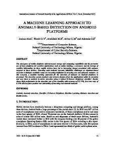
Figure 3: Count and ICD of clusters for port 80 with CD a. < 20%, b. > 80% To improve effectiveness and efficiency, CLAD learns a model for each port (application protocol). For ports that are rarely used (< 1% of the dataset), we lump them into one model: “Other.” Only clusters that are sparse or dense and distant trigger alerts. To make anomaly scores comparable across models, anomaly scores are normalized to the number of SD’s away from the average ICD. Density is not used in the anomaly score because it is not as reliable as ICD. This results from our analysis of how attacks are distributed between density and ICD on ports 25 and 80, which have the most traffic. Since we do not exact labels (attack or normal) for each data point, we rely on how DARPA/LL counts an alert as a detection of an attack [20]. We define CD (counted as detection) of a cluster as the percentage of data points in the cluster, when used to trigger an alert, is counted as a detection of an attack. This is an indirect rough approximation of the likelihood of an attack present in the cluster. We plot clusters with CD < 20% (“unlikely anomalies”) against Count and ICD in Fig. 2a and similarly for CD > 80% (“likely anomalies”) in Fig. 2b. Both Count and ICD are in log scale. As we compare the two plots, we observe that the likely anomalies occur more often in regions with larger ICD, and the opposite for unlikely anomalies with smaller ICD. The same observation cannot be made for Count. This is related to the fact that some attacks can occur in dense clusters as we explained previously. For port 80 in Fig 3, similar observations can be made. The figures also indicate that sparse or dense and distant clusters, which we use to trigger alerts, are likely to detect attacks. Furthermore, for port 80, 96% of the clusters have CD = 100% or < 9% (similarly for port 25). This indicates that most of the clusters are near homogeneous and hence our combination of feature vectors, distance function, and cluster width can sufficently characterize the data. Tbl. 3 shows the number of attacks detected by modeled learned for each port with at most 100 false alarms for the 10 days attack period in Weeks 4 and 5. The combined model detected 76 attacks, after removing duplicate detections from individual models. As mentioned perviously, the original DARPA participant with the most detections detected 85 attacks [20], which was achieved by a signature detector built by hand—unlike CLAD, which is an anomaly detector with no apriori knoweldge of attacks. Compared to
Table 3: Number of detections by CLAD (duplicates are removed in Combined) Port 20 21 23 25 53 79 80 110 111 143 Other Combined Detections 3 14 17 33 5 8 37 2 1 3 14 76 10
LEARD, CLAD detected fewer detections, but CLAD is handicapped by not assuming the availability of attack-free training data. However, we seem to detect more attacks than similar techniques [11, 29], which make similar assumptions, but we cannot claim that since the datasets are different. Further experimentation would help reduce the uncertainty.
5
Concluding Remarks
We motivated the significance of a machine learning approach to anomaly detection and have proposed two machine learning methods for constructing anomaly detectors. LERAD is a learning algorithm that can characterize normal behavior in logical rules. CLAD is a clustering algorithm that can identify outliers from normal clusters. We evaluated both methods with the DARPA 99 dataset and show that our methods can detect more attacks than similar existing techniques. LERAD and CLAD have different strengths and weaknesses, we would like to investigate more how one’s strengths can benefit the other. Different from CLAD, LERAD assumes the training data are free of attacks. This assumption can be relaxed by assigning scores to events that have been observed during training; these scores can be related to the estimated probability of observing the seen events. Unlike CLAD, LERAD is an offline algorithm, an online LERAD can update the random sample, used in the rule generation phase, with new data by a replacement strategy, and additional rules can be constructed that consider both new and old data. Different from LERAD, CLAD does not aim to generate a concise model, which can affect the efficiency during detection. We plan to explore merging similar clusters in a hierarchical manner and dynamically determine the appropriate number of clusters according to the L method [33]. Unlike LERAD, CLAD does not explain alerts well; we plan to use the notion of “near miss” to explain an alert by identifying centriods of normal clusters with few attributes contributing much of the distance between the alert and the normal centroid. We are also investigating extracting features from the payload, as well as, applying our mehtods to host-based data. Lastly, we are planning to evaluate our methods on data collected from live traffic on our main departmental server.
acknowledgments This research is partially supported by DARPA (F30602-00-1-0603).
References [1] C. Aggarwal and P. Yu. Outlier detection for high dimensional data. In Proc. SIGMOD, 2001. [2] R. Agrawal, T. Imielinski, and A. Swami. Mining association rules between sets of items in large databases. In Proc. ACM SIGMOD Conf., pages 207–216, 1993. [3] D. Anderson, T. Lunt, H. Javitz, A. Tamaru, and A. Valdes. Detecting unusual program behavior using the statistical component of the next-generation intrusion detection expert system (NIDES). Technical Report SRI-CSL-95-06, SRI, 1995. [4] F. Apap, A. Honig, S. Hershkop, E. Eskin, and S. Stolfo. Detecting malicious software by monitoring anomalous windows registry accesses. In Proc. Fifth Intl. Symp. Recent Advances in Intrusion Detection (RAID), 2002. [5] D. Barbara, N. Wu, and S. Jajodia. Detecting novel network intrusions using bayes estimators. In Proc. SIAM Intl. Conf. Data Mining, 2001. [6] M. Breunig, H. Kriegel, R. Ng, and J. Sander. Lof: Identifying density-based local outliers. In Proc. SIGMOD, 2000. [7] P. Clark and T. Niblett. The CN2 induction algorithm. Machine Learning, 3:261–285, 1989. [8] Silicon Defense. SPADE, 2001. http://www.silicondefense.com/software/spice/. 11
[9] P. Domingos and M. Pazzani. On the optimality of the simple bayesian classifier under zero-one loss. Machine Learning, 29:103–130, 1997. [10] R. Duda and P. Hart. Pattern classification and scene analysis. Wiley, New York, NY, 1973. [11] E. Eskin, A. Arnold, M. Prerau, L. Portnoy, and S. Stolfo. A geometric framework for unsupervised anomaly detection: Detecting intrusions in unlabeled data. In D. Barbara and S. Jajodia, editors, Applications of Data Mining in Computer Security. Kluwer, 2002. [12] S. Forrest, S. Hofmeyr, and A. Somayaji. Computer immunology. Comm. ACM, 4(10):88–96, 1997. [13] S. Forrest, S. Hofmeyr, A. Somayaji, and T. Longstaff. A sense of self for unix processes. In Proc. of 1996 IEEE Symp. on Computer Security and Privacy, 1996. [14] A. Ghosh, A. Schwartzbard, and M. Schatz. Learning program behavior profiles for intrusion detection. In Proc. 1st USENIX Workshop on Intrusion Detection and Network Monitoring, 1999. [15] J. Han and M. Kamber. Data Mining: Concepts and Techniques. Morgan Kaufmann, 2000. [16] K. Kendall. A database of computer attacks for the evaluation of intrusion detection systems. Master’s thesis, EECS Dept., MIT, 1999. [17] E. Knorr and T. Ng. Algorithms for mining distance-based outliers in large datasets. In Proc. VLDB, 1998. [18] C. Krugel, T. Toth, and E. Kirda. Service specific anomaly detection for network intrusion detection. In Proc. ACM Symp. on Applied Computing, 2002. [19] T. Lane and C. Brodley. Temporal sequence learning and data reduction for anomaly detection. ACM Trans. Information and System Security, 1999. [20] R. Lippmann, J. Haines, D. Fried, J. Korba, and K. Das. The 1999 DARPA off-line intrusion detection evaluation. Computer Networks, 34:579–595, 2000. [21] M. Mahoney and P. Chan. Learning models of network traffic for detecting novel attacks. Technical Report CS-2002-08, Florida Inst. of Tech., Melbourne, FL, 2002. http://www.cs.fit.edu/~pkc/papers/cs2002-08.pdf. [22] M. Mahoney and P. Chan. Learning nonstationary models of normal network traffic for detecting novel attacks. In Proc. Eighth Intl. Conf. on Knowledge Discovery and Data Mining, pages 376–385, 2002. [23] T. Mitchell. Machine Learning. McGraw Hill, 1997. [24] P. Neumann and P. Porras. Experience with EMERALD to date. In Proc. 1st USENIX Workshop on Intrusion Detection and Network Monitoring, pages 73–80, 1999. [25] T. Niblett. Constructing decision trees in noisy domain. In Proc. 2nd European Working Session on Learning, pages 67–78, 1987. [26] V. Paxon. Bro: A system for detecting network intruders in real-time. In Proc. 7th USENIX Security Symp., 1998. [27] V. Paxon and S. Floyd. The failure of poisson modeling. IEEE/ACM Transactions on Networking, 3:226–24, 1995. [28] J. Pearl. Probabilistic Reasoning in Intelligent Systems: Networks of Plausible Inference. Morgan Kaufmann, 1987. [29] L. Portnoy. Intrusion detection with unlabeled data using clustering. Undergraduate Thesis, Columbia University, 2000.
12
[30] F. Provost and P. Domingos. Tree induction for probability-based rankings. Machine Learning, 2002. [31] S. Ramaswamy, R. Rastogi, and K. Shim. Efficient algorithms for mining outliers from large data sets. In Proc. SIGMOD, 2000. [32] M. Roesch. Snort – lightweight intrusion detection for networks. In USENIX LISA, 1999. [33] S. Salvador and P. Chan. Learning states and rules for time-series anomaly detection. Technical Report CS-2003-05, Florida Inst. of Tech., Melbourne, FL, 2003. http://www.cs.fit.edu/~pkc/papers/cs-200305.pdf. [34] R. Sekar, M. Bendre, D. Dhurjati, and P. Bollinen. A fast automaton-based method for detecting anomalous program behaviors. In Proc. IEEE Symp. Security and Privacy, 2001. [35] K. Sequira and M. Zaki. ADMIT: Anomaly-based data mining for intrusions. In Proc. KDD, 2002. [36] S. Staniford, J. Hoagland, and J. McAlerney. Practical automated detection of stealthy portscans,. J. Computer Security, 2002. [37] I. Witten and T. Bell. The zero-frequency problem: estimating the probabilities of novel events in adaptive text compression. IEEE Trans. on Information Theory, 37(4):1085–1094, 1991.
13