A Memetic Algorithm with Population Management for the Generalized ...

A Memetic Algorithm with Population Management for the Generalized Minimum Vertex-Biconnected Network Problem Anna Pagacz Vienna University of Technology Favoritenstrasse 9–11/1861 1040 Vienna, Austria [email protected]

G¨unther R. Raidl Vienna University of Technology Favoritenstrasse 9–11/1861 1040 Vienna, Austria [email protected]

Bin Hu Vienna University of Technology Favoritenstrasse 9–11/1861 1040 Vienna, Austria [email protected]

Abstract—We consider the generalized minimum vertexbiconnected network problem (GMVBCNP). Given a graph where nodes are partitioned into clusters, the goal is to find a minimal cost subgraph containing exactly one node from each cluster and satisfying the vertex-biconnectivity constraint. The problem is NP-hard. The GMVBCNP has applications in the design of survivable backbone networks when single component outages are considered. We propose a Memetic Algorithm with two crossover operators, three mutation operators, and a local search component based on two neighborhood structures. Furthermore, two different population management approaches are investigated. Experimental results document the efficiency of the new approach. In particular, the local search component and the population management strategies have a substantial impact on solution quality as well as running time. Keywords-network design; biconnectivity; memetic algorithm; local search; population management

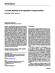
I. I NTRODUCTION The generalized minimum vertex-biconnected network problem (GMVBCNP) is defined as follows. We consider an undirected, weighted, complete graph G = (V, E, c) with node set V , edge set E, and edge cost function c : E → R+ . Node set V is partitioned into r pairwise disjoint clusters V1 , V2 , . . . , Vr . A solution to the GMVBCNP defined on G is a subgraph S = (P, T ) with P = { p1 , . . . , pr } ⊆ V and T ⊆ E connecting exactly one node from each cluster, i.e., pi ∈ Vi , ∀i = 1, . . . , r. We denote P as the set of spanned nodes. Furthermore, S may not contain any cut nodes. A cut node is a node whose removal would disconnect the graph. An example is given in Figure 1. The cost of such a vertex-biconnected network S is its total edge costs, i.e., P C(T ) = c(u, v) and the objective is to identify (u,v)∈T a feasible solution with minimum costs. The GMVBCNP appears in the design of survivable backbone networks that should be fault tolerant to a single component outage. For this problem we suggest a memetic algorithm (MA) that uses problem specific variation operators, local improvement procedures to enhance the solution quality, and population management techniques to control the diversity and to avoid over-hasted convergence.

V1

V2

p1

p2

V3

V4 p4

p3

V6 p6

V5 p5

Figure 1.

Example for a solution to the GMVBCNP.

II. P REVIOUS W ORK There are many works in the literature on to classical vertex-biconnectivity augmentation problem (VBCAP). However the generalized version is rather new. VBCAP was first investigated by Eswaran and Tarjan [1]. They showed that it is NP-hard and introduced the so-called “block-cut graph” that allows efficient detection of cut vertices. This basic principle is used here as well. From the complexity of VBCAP it directly follows that also GMVBCNP is strongly NP-hard. A similar problem is the generalized minimum edge-biconnected network problem (GMEBCNP) where only edge-biconnectivity is required. It was introduced by Huygens [6] who proposed integer programming formulations, but no practical results were published. Hu et al. [3] presented variable neighborhood search (VNS) approaches for the GMEBCNP based on several types of neighborhood structures. They are adapted for the GMVBCNP in this work. Preliminary results of the MA were published in [5], and in this article the approach is extended particularly by a new population management technique. Further details can also be found in the first author’s master thesis [8]. III. A M EMETIC A LGORITHM FOR THE GMVBCNP We use a standard memetic algorithm (MA) framework [7] for approaching the GMVBCNP as illustrated in Al-

Algorithm 2: Memetic Algorithm for GMVBCNP randomly create initial population Π repeat select two parental solutions S1 , S2 ∈ Π create a new solution Snew by crossover on S1 , S2 mutate Snew with probability pmut locally improve Snew with probability pls apply population management until no new better solution found in last l iterations

V1

V2

V1

V4

V3

V6 V5

Figure 2.

Global structure corresponding to solution in Figure 1.

V1 p2

p2 V4

V3

p4

p3

V2 p1

V4

V3

V6

p4

p3

V6

p6

V5

p5

a) Solution S1

b) Solution S2

V2

p1

V1

V2

p1

p2

V4

V3 p3

p6

V5 p5

V1

gorithm 2. Tournament selection with a size of two and a worst solution replacement strategy are used. We apply two population management techniques which can be used either separately or in combination. For the solution representation we first introduce the so-called global graph. Given a clustered graph G = (V, E, c) the global graph denoted by Gg = (V g , E g ) consists of nodes corresponding to clusters in G, i.e., V g = {V1 , V2 , . . . , Vr }, and the complete edge set E g = {(Vi , Vj ) | Vi , Vj ∈ V g , Vi 6= Vj }. Hereby, each global connection (Vi , Vj ) represents all edges {(u, v) ∈ E | u ∈ Vi ∧ v ∈ Vj } of graph G. When given some feasible candidate solution S = hP, T i to the GMVBCNP, its corresponding global structure is defined as the induced global graph’s subgraph S g = hV g , T g i with the global connections T g = {(Vi , Vj ) ∈ E g | ∃(u, v) ∈ T ∧ u ∈ Vi ∧ v ∈ Vj }. Figure 2 illustrates a global structure of the solution in Figure 1. A feasible candidate solution S = (P, T ) is characterized by P , the set of spanned nodes that are connected from each cluster, and the corresponding global structure T g containing the global connections between clusters, i.e., T g = {(Vi , Vj ) ∈ E g | ∃(u, v) ∈ T ∧ u ∈ Vi ∧ v ∈ Vj }. Using either P or T g alone is insufficient, since decoding the solution would become NP-hard subproblems. The initialization procedure for creating starting solutions is inspired by the fact that Hamiltonian cycles represent feasible solutions to the GMVBCNP: We first fix the set of spanned nodes P by randomly selecting pi ∈ Vi , ∀i = 1, . . . , r, and then connect them in random order to a cycle.

V2

p1

p2 V4

V3

p4 V6

p4

p3

V6

p6

V5

p6

V5 p5

p5

c) Solution Snew after merging edges Figure 3.

d) Solution Snew after removing redundant edges

Example for greedy crossover operator.

A. Recombination For generating a new solution Snew = (Pnew , Tnew ) from two parental solutions S1 = (P1 , T1 ) and S2 = (P2 , T2 ) we use two operators, the node-oriented crossover and the greedy crossover. A common step for both is the inheritance of spanned nodes. To determine Pnew we apply classical uniform crossover, i.e., we randomly choose the spanned node of each cluster either from P1 or P2 . Next we build g . Since the spanned nodes are the global structure Tnew g already fixed, each global connection (Vi , Vj ) ∈ Tnew now corresponds to a specific edge (pi , pj ) ∈ E, pi ∈ Vi ∧ pj ∈ Vj ∧ pi , pj ∈ Pnew . g For node-oriented crossover, Tnew is derived by visiting all clusters sequentially and for each cluster Vi ∈ g Pnew , ∀i = 1, . . . , r, we randomly decide from which parental edge set T1g or T2g the incident edges will be added. Hereby we favor the edges from the parent with lower connection cost by choosing it with probability 0.7. The resulting solution is checked by a depth-first-search algorithm and additional edges are introduced to eliminate eventually discovered cut nodes. On the other hand, greedy g crossover generates Tnew by simply merging all global g connections of both parental solutions, i.e., Tnew = T1g ∪T2g . So far, both crossover operators create solutions that in general contain more edges than needed – especially greedy crossover. Therefore, in the next step we remove edges as long as the biconnectivity constraint is not violated. During this process we consider only edges (pi , pj ) ∈ Tnew with deg(pi ) > 2 ∧ deg(pj ) > 2, where deg(pi ) denotes the degree of node pi . These edges are considered in a particular

order for removal: • α: decreasing costs 0 • β: decreasing perturbed costs c (pi , pj ) · ρ, where ρ is a uniformly distributed random value ∈ [0.5, . . . , 1.0] • γ: random order Sequence α obviously emphasizes intensification whereas γ yields a higher diversification. Each time one of the crossover operators is applied, we select the sorting criterion for edge removal randomly with probabilities (pα , pβ , pγ ). These values are initially set to (0.5, 0.3, 0.2) and dynamically adapted during the search process by the population management procedure, which observes the diversity in the current population, see Section III-D. In particular, if the diversity factor div will be too small or too high, then pγ is increased and pα decreased, respectively. Figure 3 presents an example for the greedy crossover operator. Preliminary experiments suggested to use greedy crossover with probability 0.95 and node-oriented crossover significantly less frequently with probability 0.05 since it has a much stronger heuristic bias. B. Mutation Each time a new solution Snew is generated, it is mutated with probability pmut =0.6. We have three mutation operators which introduce a small amount of randomness and ensure that all solutions in the search space have the possibility of being examined: • Change the spanned node of a random cluster. • Add a global connection between two random clusters. • Exchange the set of incident edges of two random clusters. These operators are, again according to preliminary results, applied with probabilities 0.5, 0.4, 0.1, respectively. C. Local improvement After mutation each solution is further optimized via local improvement with probability pls . In [3], a graph reduction technique has been introduced and successfully applied to the GMEBCNP, which we also use here. The motivation is to reduce the search space for some neighborhood structures which the local improvement procedures are based on. Considering the global structure, we distinguish between branching clusters having a degree greater than two and path clusters having a degree of two. Note that there are no clusters with degree one, since this would violate the biconnectivity constraint. Formally, for any global structure S g = hV g , T g i, we g g g define a reduced global structure Sred = hVred , Tred i. g Vred denotes the set of branching clusters, i.e. Vred = g {Vi ∈ V g | deg(Vi ) ≥ 3}. Tred consists of edges which represent sequences of path clusters cong necting these branching clusters, i.e. Tred = {(Va , Vb ) |

V2

V1

V2

V4

V3

V3 V6 V5

Figure 4. Example for applying graph reduction on the global structure in Figure 2.

(Va , Vk1 ), (Vk1 , Vk2 ), . . . , (Vkl−1 , Vkl ), (Vkl , Vb ) ∈ T g ∧ g g Va , Vb ∈ Vred ∧Vki ∈ / Vred , ∀i = 1, . . . , l}. Corresponding to g g g the reduced global structure Sred = hVred , Tred i we define a reduced graph Gred = hVred , Ered i with nodes representing g all branching clusters Vred = {v ∈ Vi | Vi ∈ Vred } and edges between any pair of nodes whose clusters are adjacent in the reduced global structure, i.e. (i, j) ∈ Ered ⇔ (Vi , Vj ) ∈ g Tred , ∀i ∈ Vi , j ∈ Vj . Each such edge (i, j) corresponds to the shortest path connecting i and j in the subgraph of G represented by the reduced structure’s edge (Vi , Vj ), and (i, j) therefore gets assigned this shortest path’s costs. Figure 4 shows an example for applying graph reduction on the global structure in Figure 2. V2 and V3 are branching clusters while all others are path clusters. Based on this graph reduction technique, we make use of two neighborhood structures: The Node Optimization Neighborhood (NON) emphasizes the selection of the spanned nodes in the branching clusters while not modifying the global structure. First graph reduction is carried out on the current solution S. When Vred is the set of branching clusters, NON consists of all solutions S 0 that differ from S by exactly one spanned node of a branching cluster. A move within NON is accomplished by changing pi ∈ Vi ∈ Vred to p0i ∈ Vi , pi 6= p0i , i ∈ {1, . . . , r}. By using the graph reduction technique, spanned nodes of path clusters are computed in an efficient way. The pseudocode is given in

Algorithm 3: Node Optimization (solution S) g g g compute reduced structure Sred = hVred , Tred i g forall Vi , Vj ∈ Vred ∧ Vi 6= Vj do forall u ∈ Vi 6= pi do change used node pi of cluster Vi to u forall v ∈ Vj do change used node pj of cluster Vj to v if current solution better than best then save current solution as best restore initial solution restore and return best solution

Algorithm 4: Cluster Re-Arrangement (solution S) g g g compute reduced structure Sred = hVred , Tred i for i = 1, . . . , r − 1 do for j = i + 1, . . . , r do swap adjacency lists of nodes pi and pj if Vi or Vj is a branching cluster then recompute reduced solution g g g Sred = hVred , Tred i else if Vi and Vj are in same reduced path P then g update P in Sred else g update the path containing Vi in Sred g update the path containing Vj in Sred if current solution better than best then decode and save current solution as best g restore initial solution and Sred restore and return best solution

Algorithm 3. With the Cluster Re-Arrangement Neighborhood (CRAN) we try to improve a solution with respect to the arrangement of the clusters. Given a solution S with its global structure S g = (V g , T g ), let adj(Va ) and adj(Vb ) be the sets of adjacent clusters of Va and Vb in S g , respectively. Moving from S to a neighbor solution S 0 in CRAN means to swap these sets of adjacent clusters, resulting in adj(Va0 ) = adj(Vb ) and adj(Vb0 ) = adj(Va ) with Va0 and Vb0 being the clusters in S 0 corresponding to Va and Vb in S, respectively. S 0 is further improved by performing shortest path calculations to re-choose the spanned nodes in the path clusters. Whenever two path clusters are swapped only incremental updates on the paths that contain them is necessary. In case at least one of these clusters is a branching cluster, the structure of the whole solution graph may change, and consequently the graph reduction procedure is completely re-applied. The pseudocode is given in Algorithm 4.

D. Population management Local improvement can lead to premature convergence. For this reason we apply population management in order to maintain a certain degree of diversity when new solutions are generated and added to the population. We propose two techniques. For delta management we measure the Hamming distance between the new solution Snew and each of k randomly chosen solutions in the current population Π. If the minimal distance is lower than a certain limit, Snew is mutated until the distance to the solutions in the population is sufficiently high. To save computation time the

new solution is compared only with 10% of the population, i.e. k = b0.1 · |P |c. The second technique is called edge management. It examines the percentage of the global connections covered by the solutions in the population in relation to all possible global connections. This ratio is calculated every t=50 iterations, and when it drops under a given threshold pedge < 70% then the crossover parameters (pα , pβ , pγ ) are set to (0.2,0.2, 0.6) to increase population diversity. On the other hand, when the ratio becomes higher than pedge again, these parameters are reset to (0.5, 0.3, 0.2). To conclude, if the number of covered global connections is too low, diversity is increased in the population. If it is too high, we put more emphasis on intensification. Parameters k and t control the granularity and time effort for the population management.

IV. C OMPUTATIONAL RESULTS We tested our MA on Euclidean TSPlib1 instances with geographical center clustering [2]. They contain up to 442 nodes partitioned into 89 clusters. The number of nodes per cluster varies. All experiments have been performed on an AMD Opteron Processor 2214 with 8GB RAM. The program was written in C++ and gcc version 4.1.3 was used. The stopping criterion for the MA was 200 generations without improvement of the so far best solution. In order to compute average solution values and corresponding standard deviations, 30 independent runs have been performed for each instance. In the default setting for the MA we use population size |P | = 100, local improvement probability pls = 0.2 and apply delta population management. These settings are justified by the following tests where best results are marked bold. First we vary the population size between 50, 100, 150 and 200 individuals and keep the other parameters unchanged. Results are given in Table I. Listed are average objective values of finally best solutions C(T ), corresponding standard deviations σ, and CPU-times time in seconds. We see that best results are obtained with |P | = 100 and |P | = 150. Due to population management, using a larger population size causes more computation time. This is the reason why |P | = 100 is preferred as the default value for |P |. Next we show results for different probability values of applying local improvement values in Table II. We observe that local improvement has a high impact on the solution quality as well as runtime. By comparing in particular the settings of pls = 0.2 and pls = 1.0, we see that final results were better by 1 to 5% in the latter case. However, the search process took 30% to 125% more time. Therefore the following tests have been performed with pls = 0.2 for good balance. 1 http://elib.zib.de/pub/Packages/mp-testdata/tsp/tsplib/tsplib.html

Table I R ESULTS OF THE MA FOR DIFFERENT POPULATION SIZES , WITH PROBABILITY pls = 0.2 OF APPLYING LOCAL IMPROVEMENT.

Instance Name gr137 kroa150 d198 krob200 gr202 ts225 pr226 gil262 pr264 pr299 lin318 rd400 fl417 gr431 pr439 pcb442

popsize = 50 C(T ) σ 448.5 6.0 11765.8 227.9 10869.1 152.4 13821.6 316.8 326.5 4.5 71394.7 1720.5 67992.0 1609.3 1147.0 41.3 32196.6 837.6 24409.5 628.2 22184.1 393.6 7203.2 153.4 10366.4 246.2 1316.7 17.7 63950.2 1718.7 23986 594.0

time 1.1 1.4 2.6 2.7 2.6 3.2 2.8 5.5 6.3 7.3 8.5 16.6 14.7 19.8 20.1 22.3

popsize = 100 C(T ) σ time 444.4 4.7 2.0 11809.5 289.0 2.3 10840.6 115.4 5.2 13896.5 325.1 4.5 323.1 4.9 4.7 70296.9 754.5 5.4 66939.4 1186.9 5.4 1132.3 27.2 10.4 32031.5 511.1 10.5 23801.5 682.3 14.1 21811.0 396.2 15.1 7142.8 137.5 30.5 10277.4 201.4 27.7 1306.1 13.2 36.6 62462.2 1448.1 36.4 23350.9 524.8 43.4

popsize = 150 C(T ) σ time 443.1 4.9 2.7 11744.1 275.8 3.3 10844.4 128.0 6.9 13831.3 296.0 6.3 324.1 5.2 6.3 70285.3 538.0 7.7 66905.7 950.2 7.2 1142.9 35.1 13.7 31945.2 763.2 14.8 23726.0 640.1 18.7 21785.0 477.9 22.3 7225.6 176.1 39.9 10292.3 174.1 38.2 1306.4 12.4 52.7 62259.6 1132.1 51.0 23745.3 604.9 57.4

popsize = 200 C(T ) σ time 445.6 5.3 3.0 11752.6 289.7 7.4 10889.8 156.1 7.7 13873.3 297.2 6.9 323.5 4.7 7.2 70305.6 444.2 8.7 67088.4 702.2 8.1 1154.6 33.0 15.2 32151.3 729.4 16.8 24063.4 823.5 21.0 21961.4 419.9 24.0 7234.6 182.8 47.1 10304.6 224.1 44.2 1308.7 11.4 58.6 62412.4 1008.9 57.2 24084.7 578.6 58.2

Table II R ESULTS OF THE MA FOR DIFFERENT PROBABILITIES pls OF APPLYING LOCAL IMPROVEMENT, POPULATION SIZE 100.

Instance Name gr137 kroa150 d198 krob200 gr202 ts225 pr226 gil262 pr264 pr299 lin318 rd400 fl417 gr431 pr439 pcb442

pls =0 C(T ) 476.5 12994.5 11708.1 15153.4 355.7 78642.1 75712.8 1 351.7 36185.4 29313.8 28387 9678.5 13307 1716.6 88956.3 32272.0

σ 17.8 691.1 407.8 655.9 11.0 3100.0 3632.2 102.3 1799.4 2361.7 1927.6 689.5 844.6 120.4 6915.2 2432.3

time 1.5 2.1 3.8 3.9 3.4 4.7 4.3 6.7 7.0 9.3 9.7 15.8 18.5 18.7 22.1 23.1

C(T ) 444.4 11809.5 10840.6 13896.5 323.1 70296.9 66939.4 1132.3 32031.5 23801.5 21811.0 7142.8 10277.4 1306.1 62462.2 23350.9

pls =0.2 σ 4.7 289.0 115.4 325.1 4.9 754.5 1186.9 27.2 511.1 682.3 396.2 137.5 201.4 13.2 1448.1 524.8

time 2.0 2.3 5.2 4.5 4.7 5.4 5.4 10.4 10.5 14.1 15.1 30.5 27.7 36.6 36.4 43.4

C(T ) 441.3 11619.8 10753.6 13573.2 320.0 69910.2 66687.1 1108.3 31409.1 23313.6 21562.3 6958.8 10156.3 1296.0 61284.5 22877.7

pls =0.6 σ 2.5 150.3 102.9 192.4 2.3 307.4 966.5 23.2 847.7 442.2 373.3 122.5 198.4 10.4 670.3 295.2

time 2.9 3.6 7.6 7.2 7.3 8.9 7.4 15.3 17.4 22.2 24.8 51.2 41.5 60.5 59.6 69.6

C(T ) 440.8 11601.8 10730.6 13531.6 319.7 69768.5 66126.3 1099.1 30860.8 23016.5 21368.9 6887.7 10129.1 1290.4 61132.1 22481.1

pls =1.0 σ 1.7 90.7 97.9 167.5 2.5 332.9 980.8 18.9 816.1 325.0 189.5 114.8 177.7 8.7 552.0 277.9

time 3.9 4.7 9.3 9.2 9.1 13.0 9.9 20.7 23.2 28.1 31.9 70.4 49.0 81.9 78.8 94.9

Table III R ESULTS OF MA WITH DIFFERENT POPULATION MANAGEMENT STRATEGIES , pls =0.2.

Instance Name gr137 kroa150 d198 krob200 gr202 ts225 pr226 gil262 pr264 pr299 lin318 rd400 fl417 gr431 pr439 pcb442

no management C(T ) σ time 445.8 6.3 1.8 11898.2 418.2 2.3 10836.2 125.1 4.7 13811.9 362.1 4.8 326.5 6.1 4.4 70520.5 7 65.2 5.5 66215.1 1247.7 4.8 1145.2 34.3 9.2 31765.4 940.9 9.9 24258.9 964.7 12.6 21917.6 514.2 14.3 7273.1 190.2 28.9 10193.5 291.9 26.7 1309.2 17.5 34.6 62793.0 1587.9 36.7 23473.8 633.5 42.0

delta management C(T ) σ time 444.4 4.7 2.0 11809.5 289.0 2.3 10835.2 115.4 5.2 13896.5 325.1 4.5 323.1 4.9 4.7 70296.9 754.5 5.4 66939.4 1186.9 5.4 1132.3 27.2 10.4 32031.5 511.1 10.5 23801.5 682.3 14.1 21811.0 396.2 15.1 7142.8 137.5 30.5 10277.4 201.4 27.7 1306.1 13.2 36.6 62462.2 1448.1 36.4 23350.9 524.8 43.4

edge management C(T ) σ time 446.6 6.2 2.5 11858.9 328.1 3.1 10796.3 136.8 7.6 13856.7 359.5 6.6 325.7 5.8 6.5 70127.6 430.4 8.2 66039.0 877.5 8.0 1155.3 38.9 14.0 31733.9 962.0 15.9 24284.7 883.0 19.2 21860.7 415.4 22.6 7213.8 164.2 48.0 10105.7 182.6 48.8 1305.7 13.4 57.9 62713.4 1882.5 55.3 23782.3 653.4 63.6

delta & edge management C(T ) σ time 444.4 5.2 3.9 11618.3 110.2 5.3 10798.4 124.9 12.7 13658.4 197.7 10.8 321.9 4.1 10.3 70092.1 517.6 14.4 66852.2 816.9 16.1 1140.7 31.3 26.8 31661.1 760.6 29.6 23727.3 532.6 37.7 21733.0 358.1 42.2 7081.8 149.1 82.3 10212.1 181.2 104.8 1308.2 12.5 111.9 62686.3 1716.5 56.4 24022.6 634.7 62.9

Table IV R ESULTS OF MA WITH DEFAULT CONFIGURATION AND EXTENSIVE CONFIGURATION . Instance Name gr137 kroa150 d198 krob200 gr202 ts225 pr226 gil262 pr264 pr299 lin318 rd400 fl417 gr431 pr439 pcb442

default C(T ) 444.4 11809.5 10835.2 13896.5 323.1 70296.9 66939.4 1132.3 32031.5 23801.5 21811.0 7142.8 10277.4 1306.1 62462.2 23350.9

configuration σ time 4.7 2.0 289.0 2.3 115.4 5.2 325.1 4.5 4.9 4.7 754.5 5.4 1186.9 5.4 27.2 10.4 511.1 10.5 682.3 14.1 396.2 15.1 137.5 30.5 201.4 27.7 13.2 36.6 1448.1 36.4 524.8 43.4

extensive C(T ) 441.6 11631.4 10716.0 13646.2 321.8 69706.9 65468.5 1127.7 30662.5 23424.8 21517.0 7163.6 10091.8 1300.5 61654.0 23011.6

configuration σ time 2.7 8.3 155.4 10.3 100.9 24.9 245.8 22.2 4.5 21.1 418.8 28.9 966.2 27.8 22.3 49.3 638.2 58.3 865.0 77.6 318.2 88.8 173.9 176.1 160.6 171.1 13.6 239.1 817.3 233.7 430.2 155.1

Table III lists results for different settings of the population management. It documents that population management is highly effective w.r.t. solution quality. Obtained results are in most cases significantly better when at least one of the strategies is turned on and usually best when both are applied. On the other hand, when both strategies were active, running times also increased considerably. Finally, in Table IV we compare results between the default setting and an “extensive” configuration where all parameters are set towards best results, i.e., |P | = 200, pls = 1.0, and both population management strategies activated. We see that although the extensive configuration yields in general better results, the computation times increase enormously. Surprisingly, these results are not significantly superior to those when parameters are tuned for best results one at a time, compare to the last columns of Table II and III. In order to compare the MA with an exact approach based on integer programming, we derived a multi-commodity flow Mixed Integer Programming (MIP) model from the GMEBCNP [3] by further adding constraints to guarantee vertex-biconnectivity. Due to space reason the full MIP formulation is not given here. Based on this model, by using the general purpose MIP solver CPLEX in version 11.2 we were able to obtain optimal solutions within reasonable time for small instances with up to around 80 nodes. However, the practical limit is quickly reached when the problem size increases. Since benchmark instances used in this article have at least 137 nodes, it was not possible to obtain optimal solutions anymore.

V. C ONCLUSIONS AND F UTURE W ORK In this paper we considered the minimum vertexbiconnected network problem (GMVBCNP). We developed

a memetic algorithm (MA) with advanced crossover operators, local improvement methods, and two population management techniques. The parameters for crossover are adapted dynamically during the search process by population management. Best results were obtained when local improvement is always applied, but the computation time then also grows. Two different population management strategies, which can be either used together or separately, have been investigated as well. Performed experiments clearly indicate that better results are obtained when both are used, but this configuration again requires more computation time. Future work should include more comprehensive tests also on other types of instances, e.g., Euclidean instances with random clustering or non-Euclidean instances. Other types of genetic operators might also be promising, e.g., an edgeoriented crossover that keeps the edges but re-selects nodes. On the other hand, the mixed integer program formulation can be further developed and a hybridization with MA could also be done like in [4].

R EFERENCES [1] K. P. Eswaran and R. E. Tarjan. Augmentation problems. SIAM Journal on Computing, 5(4):653–665, 1976. [2] C. Feremans. Generalized Spanning Trees and Extensions. PhD thesis, Universite Libre de Bruxelles, Brussels, Belgium, 2001. [3] B. Hu, M. Leitner, and G. R. Raidl. The generalized minimum edge biconnected network problem: Efficient neighborhood structures for variable neighborhood search. accepted for Networks. [4] B. Hu, M. Leitner, and G. R. Raidl. Combining variable neighborhood search with integer linear programming for the generalized minimum spanning tree problem. Journal of Heuristics, 14(5):473–499, 2008. [5] B. Hu and G. R. Raidl. A memetic algorithm for the generalized minimum vertex-biconnected network problem. 9th International Conference on Hybrid Intelligent Systems - HIS 2009, pages 63–68, 2009. [6] D. Huygens. Version generalisee du probleme de conception de reseau 2-arete-connexe. Master’s thesis, Universite Libre de Bruxelles, 2002. [7] P. Moscato and C. Cotta. A gentle introduction to memetic algorithms. In F. Glover and G. Kochenberger, editors, Handbook of Metaheuristics, pages 105–144. Kluwer Academic Publishers, Boston MA, 2003. [8] A. Pagacz. Heuristic methods for solving two generalized network problems. Master’s thesis, Vienna University of Technology, Institute of Computer Graphics and Algorithms, February 2010. supervised by G. Raidl and B. Hu.