International Journal of Computational Intelligence Research. ISSN 0973-1873 Vol.3, No.3 (2007), pp. 219-229 © Research India Publications http://www.ijcir.info
A Method to Edit Training Set Based on Rough Sets Yailé Caballero1, Rafael Bello2, Yanitza Salgado1 and María M. García2 1
Department of Computer Science. University of Camaguey, Cuba
[email protected]
2
Department of Computer Science. Universidad Central de Las Villas, Cuba {rbellop, mmgarccia}@uclv.edu.cu
Abstract: Rough Set Theory (RST) is a technique for data analysis. In this paper, we use RST to improve the performance of the k-NN method and the MLP neural network. The RST is used to edit the training set. We propose two methods to edit training sets, which are based on the lower and upper approximations. Experimental results show a satisfactory performance of the k-NN method and MLP using these techniques. Keywords: k-NN method, MLP, Rough Set Theory, data analysis, edit training set.
I. Introduction Machine learning is an important area inside Computer Science. Generally, this is a process that consists of use training sets in order to obtain knowledge automatically about it, and according to the results it could be classified into lazy or inductive learning. An example of lazy learning is the IBL and an inductive one is the Multilayer Perceptron Artificial Neural Network. A major goal of Machine learning is the classification of previously unseen examples. Beginning with a set of examples, the system learns how to predict the class of each one based on its features. The selection of examples from a domain to include in a training set is a present problem in all of the computational models for learning from examples. This is known as the edition of training sets. Instance-based learning (IBL) is a machine learning method that classifies new examples by comparing them to those already seen and are in memory. This memory is a Training Set (TS) of preclassified examples, where each example (also called object, instance or case) is described by a vector of features or attributes values. A new problem is solved by finding the nearest stored example taking into account some similarity functions; the problem is then classified according to the class of its nearest neighbor.
Nearest neighbor methods regained popularity after Kibler and Aha showed that the simplest of the nearest neighbor models could produce excellent results for a variety of domains. A series of improvements was introduced in the IB1 to IB5 [1]. IBL method is often faced with the problem of deciding how many exemplars to store, and what portion of the instance space it should cover. An extension to the basic IBL paradigm consists in using the K nearest neighbors instead of just the nearest one, the class assigned is that of the majority of those K neighbors, taking into account the distance (or similarity) between the problem and each nearest neighbor [2]. There are many Artificial Neural Network models that had been used in classification problems, such as: McCulloch and Pitts, Perceptron, Multi-Layer Perceptron (MLP), Adaline, Madaline, Hamming net, among others. MLP is recognized as the best artificial neural network used in classification from examples. The presence of mistaken labeled prototypes in the training set is a problem that affects seriously the efficiency of the classification methods. There are some problems that can occur during the training such as mistakes while labeling the prototypes or noisy patterns that can appear due to troubles while getting the data. These prototypes appear usually in zones near the decision region and have a negative influence in the learning process, because it increases the error rate of the classification. Besides, there is a high computational cost associated to the application of classification methods to the whole set of prototypes. A functional scheme of classification that takes as reference set an edited set (SE) and the whole set of prototypes (S) is shown in Figure 1. SE is a prototypes edited set, and it had been built from S through some edition method. R indicates the reference set that is used in the classification method. [3].
220
Yailé Caballero et al
Figure 1. Classification’s Schema. Data reduction is realized in two directions. First one consists of the reduction of the attribute quantity that is used to describe the objects. The second one is the decrease of the objects quantity to include in the training set. Rough Set Theory (RST) has been an excellent mathematical tool for data analysis and it has offered an exciting theoretic base for the solution of many problems within knowledge discovery [4], [5], [6], [7], [8], [9] and [10]. Several toolkits based on rough sets to data analysis have been implemented, such as Rosetta [11] and [12], and ROSE [13]. Rough Sets theory was proposed by Z. Pawlak in 1982 [14]. The rough set philosophy is founded on the assumption that some information is associated with every object of the universe of discourse [15] and [16]. A training set can be represented by a table where each row represents objects and each column represents an attribute. This table is called Information System; more formally, it is a pair S= (U, A), where U is a non-empty finite set of objects called the Universe and A is a non-empty finite set of attributes. A Decision System is any information system of the form SD=(U, A∪{d}), where d∉A is the decision attribute. Classical definitions of lower and upper approximations were originally introduced with reference to an indiscernible relation which assumed to be an equivalence relation. Let B⊆A and X⊆U. B defines an equivalence relation and X is a concept. X can be approximated using only the information contained in B by constructing the B-lower and B-upper approximations of X, denoted by B*X and B*X respectively, where B*X={ x : [x]B ⊆X } and B*X={ x : [x]B ∩ X≠φ }, and [x]B denotes the class of x according to B-indiscernible relation. The objects in B*X are sure members of X, while the objects in B*X are possible members of X. Rough set model has several advantages to data analysis. It is based on the original data only and does not need any external information; no assumptions about data are necessary; it is suitable for analyzing both quantitative and qualitative features, and the results of rough set model are easy to understand [17]. An important issue in the RST is about feature reduction. All the computational models that realize inferences from examples have the problem of the selection of the examples from the domain that must be included in the training set.
This problem in known as the training sets edition. The object reduction techniques pursue as objective the elimination of patterns or prototypes for decreasing the size of the learning matrix. It is about decreasing the computational work and, at times, it is disposed or ready to pay with a little less precision of the system, but with more computational efficiency. The Editing techniques are applied to eliminate the prototypes that induce an incorrect classification, even though it is certain that they produce elimination of prototypes, their fundamental objective is to obtain a training sample of better quality to have a better precision with the system. The aspects that have the most interest in the k-NN method are the reduction of the classification error and the reduction of the computational cost. The k-NN method is very sensitive to the presence of incorrectly labeled examples or objects close to the decision’s boundary; incorrect instances are liable to create a region around them where new examples will also be misclassified [1], [4], [5] and [6]. Moreover, the search for the nearest neighbour can be a very costly task, above all, in high dimension spaces. A major problem of instance-based learners is that classification time increases as more examples are added to training set (TS). The use of rough set in editing training sets is analyzed in this paper. In section II, we study the editing training sets. Two methods for editing training set based on the lower approximation and upper approximation concept are presented in section III. Experimental results show a satisfactory performance of k-NN using these techniques in section IV. A form to ratify with another model the edition possibilities based on approaches, is the use of a neural network, specifically a MLP was used, this experimental results are in section V.
II. Techniques for Editing and Reducing Training Sets In [18] appears one of the first attempts of reduce the size of training sets. This algorithm is especially sensitive to noise, because the noisy cases will be usually bad classified by its neighbours and will be kept. This situation causes two problems: The first is that the reduction of the storage is prevented because the noisy cases are retained. The second problem is that the exactitude of the generalization is debilitated because the noisy cases, usually the exceptions, will cover more space than in the input, and that could cause more mistakes in classification than before the reduction. Aha in [1], [19] presented some Instance-based Learning algorithms that use sample models, each concept is represented by sample set, each sample could be an abstraction of the concept or an individual instance of the concept. Between these algorithms are the following ones:
A Method to Edit Training Set Based on Rough Sets IB1: IB1 (Instance Based learning algorithm 1) was the 1-NN algorithm and was used as bottom line. IB2: IB2 is an incremental algorithm. Kibler and Aha in [20] had called this the Growth Algorithm. This one is similar to the Hart Condensed NN, but IB2 don’t build the S set with a case of each class and don’t repeat the process after the first step through the training set. Mean that IB2 won’t classify correctly all the cases in T. This algorithm retains the border points in S while deleting the inner points that surround it by the same class members. Like the CNN, IB2 is highly sensitive to noise, because the noisy cases usually will be bad classified and often will be saved on that way while the more trusted cases will be deleted. Shrink algorithm Kibler and Aha in [20] also presented an algorithm that starts with S=T and deletes any case that could be still classified correctly by the remaining subgroup. The idea is similar to the Reduced Nearest Neighbor rule (RNN), but in this case the algorithm consider if the deleted instance could be classified correctly, while the RNN takes into account if the other instances classification could be damaged by the elimination of those instances. IB3: IB3 is another incremental algorithm that try to solve the IB2 problem of save noisy cases by retaining only cases bad classified but acceptable. IB3 has reduced noise sensitivity. IB4: In order to attend some no relevant attributes, Aha in [19] extends the IB3 algorithm to the IB4 one through the construction of a set of attribute weights for each class. This requires fewer cases to obtain a good generalization when there are irrelevant attributes in a dataset. IB5: Aha in [19] also extends the IB4 to manage the addition of new attributes to the problem after the training had begun. TIBL: Zhang in [21] used a different approach that was called Typical Instance Based Learning (TIBL). TIBL algorithm tried to save instances near the center instead of the border ones in order to obtain a more drastic reduction in the storage and more smooth decision limits. The algorithm is more robust in presence of noise. MCS: Brodley in [22] introduce a Model Class Selection (MCS), this is a system which uses a learning algorithm bases in instances (that pretends to be near to IB3) and it is part of a greater hybrid learning algorithm. It trends to avoid noise. Random Mutation Hill Climbing: Skalak in [23] used the Random Mutation Hill Climbing with the purpose to select the cases to use in S. This method solves part of the problem.
221 Encoding Length (ELGrow): Cameron-Jones in [24] used a heuristic of codification length to determine how good could be the S set to describe T. This algorithm isn’t incremental, but to distinguish from other techniques it’s called Growing Encoding Length algorithm or El_Grow. Explore Cameron-Jones in [24] also presents the Explore method that begins by growing and pruning S by the use of El_Grow method. Generalization of the Explore precision method is empirically strong and its storage reduction is better than most of the other algorithms. In [25], [26], [27], [28], [29] and [30] appear various techniques of reducing the training sets, with the purpose of reducing the training sets based on the nearest neighbor theory. Six new methods called DROP 1-5 and DEL are reported in [27] which can be used to reduce the number of instances in the training sets. Editing algorithms from the training sample are described in [31], which are focused on the detection and elimination of noisy or atypical patterns in order to improve the classification’s exactitude. Some of these are ENN (Wilson in 1972), All k-NN (Tomek in 1976) and Generalized Editing Algorithm (Koplowitz and Brown in 1978). Another editing method is Multiedit Algorithm (Devijver and Kittler in 1980) [32]. Wilson in 1972 developed the Edited Nearest Neighbor (ENN). This technique consists in applying the k-NN (k > 1) classifier to estimate the class label of every prototype in the training set and discard those instances whose class label does not agree with the class associated to the majority of the k neighbors. The benefits –improvements of the generalization accuracy- of Wilson’s algorithm have been supported by theoretical and empirical evaluations [31]. In this algorithm S starts out the same as T, and then each instance in S is removed if it does not agree with the majority of its k nearest neighbors (with k=3, typically). This edits out noisy instances as well as close border cases, leaving smoother decision boundaries. It also retains all internal points, which keeps it from reducing the storage requirements as much as most other reduction algorithms. The Repeated ENN (RENN) applies the ENN algorithm repeatedly until all instances remaining have a majority of their neighbors with the same class, which continues to widen the gap between classes and smoothes the decision boundary. Tomek in 1976 extended the ENN with his All k-NN method of editing. This algorithm works as follows: for i=1 to k, flag as bad any instance not classified correctly by it’s i nearest neighbors. After completing the loop all k times, remove any instances from S flagged as bad. In his experiments, RENN produced higher accuracy than ENN, and the All k-NN method resulted in even higher accuracy yet. As with ENN, this method can leave internal points
222 intact, thus limiting the amount of reduction that it can accomplish. These algorithms serve more as noise filters than serious reduction algorithms. Koplowitz and Brown in 1978 obtained the Generalized Editing Algorithm. This is another modification of the Wilson’s algorithm. Koplowitz and Brown were concerned with the possibility of too many prototypes being removed from the training set because of Wilson’s editing procedure. This approach consists in removing some suspicious prototypes and changing the class labels of some other instances. Accordingly, it can be regarded as a technique for modifying the structure of the training sample (through relabeling of some training instances) and not only for eliminating atypical instances. In 1980 the Multiedit algorithm by Devijver and Kittler emerged. In each iteration of this algorithm, a random partition of the learning sample in N subsets is made. Then the objects from each subset are classified with the following subset applying the NN rule (the nearest neighbor rule). All the objects that were classified incorrectly from the learning sample in the previous step are eliminated and all the remaining objects are combined to constitute a new learning sample TS. If in the last I iterations no object has been eliminated from the learning sample, then end with the final learning sample TS. On the contrary, return to the initial step. We have studied the performance of these algorithms when we use k-NN methods. The results are shown in table 1. There are different aspects that characterize the editing and reducing techniques of examples, such as: Representation: It is necessary to decide if a subset of the original instances is retained or if it is modified using it to create a new representation. Direction of the search of instances: The construction of the subset S from the training set E can be done in an incremental form (begin with S being empty and start adding cases according to some criteria), a decrement form (begin with S=E and starts eliminating examples from S according to some criteria) or in batches (decide if each instance complies with the elimination criteria before separating any of them). Type of points of the space to retain: The set of cases forms a universe divided into regions, which you can have as a criteria to retain the instances situated in the boundaries of the regions, those that are situated in the center or in the interior of the regions, or another set of points. Volume of the reduction: One of the objectives of the elimination of examples is to reduce the necessary stored memory. Increment of speed: Another objective is to increase the processing velocity starting from the set of instances. Typically a reduction of the amount of examples will produce a decrease of the processing time.
Yailé Caballero et al Precision of the generalization: The success of the reduction algorithm is to be able to reduce the number of instances without significantly reducing the capacity of generalization of the processing of the algorithm. Tolerance to noise: The reduction algorithms are also different in respect to their effectiveness in the presence of noise in the data. Learning of speed: The ideal is to have a complexity of O(n2) or faster. Incremental growth: After obtaining the set S from E it should be possible to decide in an incremental form the addition of new instances to the training set while these are being obtained.
III. Rough Sets Theory in Training Sets Edition Rough Sets Theory provides efficient tools to work with this solution choices. Rough Sets Theory makes possible to try as many quantitative data as qualitative one, and there is no need to eliminate the inconsistencies previous to analysis. Another advantage of this approach is that the output information could be used to determine the attribute relevance and to generate relations among them (in rule forms). Besides, there is no need to make suppositions about the attribute independence neither other knowledge about data nature [33]. Besides, multiple applications had been developed by using Rough Sets Theory [34], [35]. A. Two methods for editing training set based on rough sets There are two important concepts in Rough Sets Theory: Lower and Upper Approximation of decision systems. Lower approximation group’s objects that certainly belong to its class, this guarantee that object inside lower approximation have no noise. We have studied the application of rough sets for the edition of training sets. We propose two methods for editing training sets by using upper and lower approximations. First, we use the lower approximations of classes to create the edited training set. The basic idea of employing rough sets for editing training sets is the following: in the training set we put the examples of the initial decision system that belong to the lower approximation of each class, that is, given an application’s domain with m classes and the equivalence relation B, then, TS = B*(D1) ∩ B*(D2) ∩ ... ∩ B*(Dm) This is equivalent to saying that the training set will be the positive region of the decision system. In this manner, objects that are incorrectly labeled or very near to the decision’s boundary can be eliminated from the training set which affect the quality of the inference/deduction. Studies on multiediting presented in [36] show that isolated objects
A Method to Edit Training Set Based on Rough Sets included in other regions or near to the decision’s boundary are frequently eliminated. Edit1RS Algorithm: Step1. Construct the set B, B⊆A. Preferably, B is a reduct from the decision system. Step2. Form the sets Xi⊆U, such that all the elements of the universe (U) that have value di in the decision’s attribute is in Xi. Step3. For each set Xi, calculate its lower approximation B*(Xi). Step4. Construct the edited training set as the union of all the sets B*(Xi). In the second case, we use lower approximations and boundary region of classes to create the edited training set. In the Edit1RS method only the elements which to the lower approximations are taken into account. Also, it is important to also take into consideration those elements that are in the boundary (BNB). The Generalized Editing Algorithm consists of removing some suspicious prototypes and changing the class labels of some other instances. Accordingly, it can be regarded as a technique for modifying the structure of the training sample (through re-labeling of some training instances) and not only for eliminating atypical instances [31]. The second algorithm is proposed taking into account these ideas. Edit2RS Algorithm: Step1. Construct the set B, B⊆A. Preferably, B is a reduct from the decision system. Step2. Form the sets Xi⊆U, such that all the elements of the universe (U) that have value di in the decision’s attribute is in Xi. Step3. S = ø Step4. For each set Xi do: Calculate their lower approximation (B*(Xi)) and upper approximation (B*(Xi)). S = S U B*(Xi). Ti = B*(Xi) - B*(Xi). Step5. Calculate the union of the sets Ti. T = U Ti is obtained. Step6. Apply the Generalized Editing method to each element in T and the result is the set T’. Step7. S = S U T’. The edited training set is obtained as the resultant set in S. The computational complexity of our algorithms don't surpass O(ln2), near to the ideal value of O(n2), while in the rest of the algorithms it is of O(n3).The Edit1RS and Edit2RS algorithms based on the rough set theory are characterized in the following way: Representation: Retain a subset of the original instances. In the case of the Edit2RS algorithm, this can change the class of some instances. Direction of the search of the instances: The construction of the subset S from the training set E is achieved in batch form. In addition, the selection is
223 achieved on a global vision of the training set not separated by decision classes. Type of point of the space to retain: The Edit1RS algorithm retains the instances situated in the centre or interior of the classes. The Edit2RS algorithm retains these instances and others included in the boundary regions of the classes. Volume of the reduction: The volume of the reduction depends on the amount of inconsistencies in the information system; there will always be a reduction in the training set, except if the information system is consistent. Increment of speed: On decreasing the amount of examples the velocity of the next processing is increased. Precision of the generalization: In the majority of cases, one of the algorithms or both of them increased significantly the efficiency of the k-NN method. Tolerance to noise: The rough set theory offers a pattern oriented to model the uncertainty given by inconsistencies, for which it is effective in the presence of noise. In fact, the lower approximation eliminates the cases with noise. Learning speed: The computational complexity of finding the lower approximation is O(ln2), according to [34] and [37], near to the ideal value of O(n2), and less than that of the calculation of the coverage (O(n3)), so l (amount of attributes considered in the equivalence relation) is in the majority of the cases significantly smaller than n (amount of examples). Incremental growth: This is an incremental method so for each new instance that appears it is enough to determine if it belongs to some lower approximation of some class so that it can be added or not to the training set. In section VI the experimental results of these methods are shown.
IV. k-NN method and Experimental results The k Nearest Neighbor Algorithm is based on lazy learning and uses a distance or similarity function to generate predictions from stored instances. It is called lazy because it stores the training set y left all the processing for the classification stage. The input of the classifier is an instance q of an unknown class. Each instance
x = {x1 , x 2 ,..., x|F | }
is a point that belongs to multidimensional space defined by the attribute set and the F class of the instance x, inside the class set J. The attribute could be from many types: real, integer, ordered symbolic, symbols sets, boolean or fuzzy. The mistake that can be made in the classification of the instances of the training sets is known as Leaving One Out Classification Error (LOOCE). The purpose of the classifier is to minimize LOOCE coefficient. The way to calculate it depends on if the class value is continuous or discrete. With discrete values, it is calculated as:
224
Yailé Caballero et al
LOOCE =
∑ ∑ (δ
q∈BC j∈J
q, j
− pq , j )
This means, for each instance q that belongs to the base cases and for each class that belongs to the class set J, it is calculated the sum of the difference between the class membership function
pq , j
δ q, j
and the class probability function
defined as:
1 qc = j δ q, j = 0 qc ≠ j pq , j =
∑ δ ⋅ sim(q, r ) ∑ sim(q, r )
2
r, j
r∈K
2
r∈K
Where
K is the more similar neighbour instance set.
When working with classes with continuous values, LOOCE is defined as: LOOCE =
∑ (q
q∈BC
qc
Where as: pq =
c
− pq ) 2
is the class of instance
∑ r ⋅ sim(q, r ) ∑ sim(q, r )
q and pq is defined
2
c
r∈K
2
r∈K
rc
Is the class value of instance r . The classification of instance using k-NN implies to
q
and the algorithm previously know the class value of returns the most probable class using the following formulas: If the class value is discrete, k-NN returns: qc = max pq , j j∈J . If the class value is continuous, k-NN returns:
qc = pq
. The similarity between two instances is calculated as:
The results that are shown in Table I allow you to compare the efficiency reached by the k-NN method using the original data bases, and the edited ones using various methods from the edition of training sets algorithms proposed by other authors and the two which are presented in section III. We have considered two alternatives: (i) B uses all features; (ii) B is a reduct. The LOOCE value was 10. A reduct is a minimal set of attributes from A that preserves the partitioning of universe (and hence the ability to perform classifications) [7]. We have used heuristic methods to calculate reducts which decrease the computational complexity [38] and [39]. By comparing the two methods based on the Rough Set Theory the superior results obtained by the Edit2RS method are appreciated. In order to verify efficiently the described results previously the statistical test of Crossed Validation was applied, for which each data set in 5 samples was divided, at every moment 4 of them were taken to train and the other to classify, so that each one of these sets was taken to classify in one of the 5 experiments of the same There 20 were made run by each one of these experiments, table 1 represents the values of the average of the 100 values of effectiveness in the classification for the test of Validation Crossed for the bases including and each one of the exposed algorithms. A Student Test was applied to Cross Validation results and the p-value obtained was less than 0.05 for each one of the topics to demonstrate: i) The results of Edit2RS method were better in classification than Edit1RS one, and ii) Efficiency percents in classification for Edit1RS and Edit2RS methods were better by using a reduct than working with all the features. It’s possible to state that there are significant differences between the results obtained by Edit1RS method and Edit2 RS one. The two methods based on the Rough Set Theory show superior behavior to those results obtained without editing. The achieved results with Edit1RS and Edit2RS are similar to those achieved by the ENN, Generalized Editing method, Multiedit method and All-KNN methods.
n
sim(q, c ) = ∑ wa ⋅ sima (q a , c a ) a =1
sima is a function of similarity used to compare a value for each instance n is the attribute wa a
Where the attribute
amount and the weight of attribute . We have study the computational behavior of the algorithms when they are employed in the k-NN method. We have used decision systems constructed from the data bases that were found in: http://www.ics.uci.edu/~mlearn/MLRepository.html
V. MLP Neural Network and Experimental Results The Multilayer Perceptron is an artificial neural network model that simulates one of the human nervous system functions: classification by using structural and functional simulation of part of that system [40]. The MLP presents a multilayer topology with continuous neuron model and the backpropagation algorithm as learning method.
A Method to Edit Training Set Based on Rough Sets
225
Table 1. Results of the classification Effectivity with k-NN Edited data set
Name of data base Ballons Breast_ Cancer Bupa Dermato logy Ecoli Hayes_ Roth Heart Iris Lung Cancer Pima Yeast
Original data bases
ENN
All_KN N
Generalize d Edit
Multi_ edit
59.23
59.23
100.00
80.40
100.00
90.40
100.00
100.00
100.00
96.77
96.24
95.69
93.26
100.00
98.00
100.00
99.35
99.65
67.83
88.74
88.11
84.98
100.00
82.16
89.93
90.23
90.47
97.49
94.56
100.00
93.14
50.00
96.46
98.78
98.27
99.19
76.61
81.54
91.89
96.49
95.71
98.28
98.06
97.70
100.00
23.48
70.37
66.66
22.11
100.00
85.29
100.00
70.27
84.62
82.22
89.54
98.40
96.11
100.00
92.37
93.50
95.41
97.31
94.66
100.00
100.00
92.66
100.00
98.94
100.00
100.00
98.66
47.34
51.00
73.28
54.00
0.00
78.00
82.29
71.00
83.02
73.05
80.00
80.00
90.36
90.36
94.33
96.64
95.43
100.00
59.03
71.43
70.00
81.75
91.01
90.03
93.76
90.00
99.74
The network must be trained first with a training set. At the end of the training, it will be ready to recognize the learned samples and to classify other new ones based on generalizations made from the training set. The MLP is used with an activation function that is evaluated with an input vector of real components that identifies a certain pattern, “analyses” it and returns the class or pattern that belongs to the vector. During the training process, the MLP learns with the samples that receive and classify every input of the training set and in dependence of the amount of error it will rectify itself in order to improve the next execution of the same sample. The process of classify all the samples will be repeated until a stopping criteria will be satisfied. Training sets are very different and the networks must learn it, also during the process some parameters are needed with the purpose of adjust the algorithm to the features of the each set and each network. The arguments that establish boundaries during the MLP training are: • Stopping criteria This parameter indicates when the training must be stopped. There are many criteria to consider the end of the learning process by the network: 1.-Generalization. In each iteration, the network optimizes
EDIT1RS B=All B=Reduct features
EDIT2RS B=All B=Reduct features
and estimates the generalization error computed from the validation set until this one reaches a value less than a specified quantity. 2.-Percent of samples learned. The network had learned a case when it is classified with an error less than the permissible one during the learning process. The network will stop the training when it had learned a percent of the specified training set. 3.- Quantity of learned samples. The training stops when the network had learned a specific number of samples. 4.- Number of iterations. The network will evaluate the training set by a specific number of iterations in which the error will be also rectified. • Learning speed The learning speed is a parameter used during training. Usually is situated between 0.5 and 0.025. While it reaches higher values, the training will be shorter. • Initial weight influence The value of this parameter usually oscillates between 0.1 and 0.8. The initial weight improves the learning process because they allow noticing last changes made over the network. It is proportional to the learning speed. • Classification error This parameter indicates the error that allows to the network when classifying an example him of the training set,
226 so that it considers that has been learned it. This parameter is very important then in dependency of same the network will make an effort more in learning or no. If the classification error value is a big number, then the learning will be fast, but the MLP will take a vague idea of each pattern and so when classifying patterns that have not appeared to him during the training can that does it of incorrect way. • Feature selection criteria During the training the network selects the simples from the training set that it will try to learn. There are three ways to select these examples: 1.- Uniform: In this kina of selection, each pattern is selected in a random way, but the probability of to be selected is the same in each pattern. This strategy is the simplest one; but it has as an inconvenient that the progress or level of the learning reached in each moment is ignored. It seems to be that this blind selection causes a non favorable chaos in the update of the weights, because does not consider at no moment nor the characteristics of the pattern who is analyzing itself, nor the error that when classifying it has been committed throughout the training. For this reason, this strategy could be a slow training process and even, it can oscillate near the minimum. 2.- Sequentially: The samples are selected in the same order that the appear in the training set. This form to take the patterns does not consider the advances that the network makes in specific patterns and causes that certain inertia in the pick up of the knowledge is created. It is little advisable to use this technique, unless the order of the examples in the training set is not accidental, but totally intentional and thought. 3.-Repeat until learn. This strategy is of the type of pedagogical selection. Each sample is presented to the network. Each example is presented to the network in dependency of the error that this one comet when classifying it. Each simple is randomly selected and repeated until its error is lower than the medium error of the network increased in a determined factor. Usually, it happens when the classification error is greater than 150% of the medium error. A MLP artificial neural network was used in a similar way to the k-NN method but to obtain effectively classification percents for each of the edited sets; results are shown in graphic 1. The parameters used with the MLP were: the stopping criteria were a generalization error of 0.02, the learning speed 0.05, the weight influence 0.5 and feature selection criteria of repeat until learn. The results with Edit1RS and Edit2RS were the best obtained when classifying the non edited training set; also, the new method returned similar results in some cases and
Yailé Caballero et al superior to the ENN, All KNN, Generalized Edition and Multiedit methods in other cases. A comparison between Edit1RS and Edit2RS was made and Edit1 RS attending to the results and the Edit2RS ones were the best. It was demonstrated that the effectivity of the new methods is superior when a reduct is used than when all features are used.
Graph 1. Efficiency reached by the MLP In order to verify efficiently the described results previously the statistical test of Crossed Validation was applied, for which each data set in 5 samples was divided, at every moment 4 of them were taken to train and the other to classify, so that each one of these sets was taken to classify in one of the 5 experiments of the same. We made 20 run by each one of these experiments, table 2 represents the values of the average of the 100 values of effectiveness in the classification for the test of Validation Crossed for the bases including and each one of the exposed algorithms. The classifier used in this experimentation was a MLP. A Student test was made to the results obtained with the Crossed Validation Test and the p value for this was less than 0.05 for each of the aspects to demonstrate. This is a good reason to affirm that there are significant differences for this bases and it could be said that: Edit1RS and Edit2RS methods show better results in classification than the training set without editing. The results obtained in training sets by Edit1RS and Edit2RS were in most of the cases superior to the ENN, All KNN, Generalized Edition and Multiedit methods. Edit2RS method had better results in classification than Edit1RS one. For the methods Edit1RS and Edit2RS the percents of effectiveness in the classification were better using a reduct than working with all the attributes.
A Method to Edit Training Set Based on Rough Sets
227
Table 2. Results using MLP when applied cross validation test Edited data set
Name of data base
Origin al data bases
ENN
All_KN N
Generalize d Edit
Multi_ edit
Ballons
58.33
53.23
100.00
78.00
100.00
90.00
100.00
100.00
100.00
Breast_ Cancer Bupa
93.20
97.89
98.13
96.56
100.00
98.69
99.00
97.33
99.89
60.45
83.33
82.54
84.01
100.00
87.25
89.15
85.00
92.00
Dermatology
92.00
94.37
98.45
99.18
100.00
95.47
96.90
98.00
99.27
Ecoli
66.87
97.71
97.89
95.27
100.00
83..23
95.19
97.56
98.00
Hayes_ Roth Heart
20.19
68.90
70.01
18.00
100.00
85.00
100.00
50.00
85.00
80.45
92.00
95.87
95.00
50.00
94.57
96.98
95.00
97.78
Iris
93.22
100.00
93.10
96.45
100.00
99.00
100.00
100.00
100.00
Lung Cancer
45.98
50.00
74.12
53.98
0.00
50.00
80.00
50.00
84.08
Pima
72.00
93.25
93.45
92.90
100.00
80.00
80.00
94.91
98.09
Yeast
55.00
91.90
93.55
90.00
96.10
70.40
70.00
92.00
97.00
EDIT1RS B=All B=Reduct features
EDIT2RS B=All B=Reduct features
VI. Conclusion
References
A study of the possibility of applying the elements of the Rough Set Theory in data analysis when the k-NN method and neural network MLP are used was presented in this paper. Two methods for the edition of training sets are proposed. Experimental results show that using rough sets to construct training sets to improve the work of the k-NN method and MLP are feasible. Our methods obtained similar results to the methods with high performance and these obtained the best result in some case. Therefore, we think these new methods can be taking into account for editing training sets in k-NN method and neural network MLP. The results obtained with the Edit1RS and Edith2RS methods were higher in the majority of cases when B is a reduct. The computational complexity of our algorithms don't surpass O(ln2), near to the ideal value of O(n2), while in the rest of the algorithms it is of O(n3).
[1] Aha, D.W. “Case-based Learning Algorithms”. Proceedings of the DARPA Case-based Reasoning Workshop. Morgan Kaufmann Publishers. 1991. [2] García Zaldívar, José M. “KNN Workshop. Suite para el Desarrollo de Clasificadores Basados en Instancias”. Trabajo de Diploma. Universidad Central "Marta Abreu" de Las Villas. Facultad de Matemática, Física y Computación. 2003. [3] Suárez-Inclán Rivero, Yadilka. Rodríguez Vallejo, Lester. Análisis del uso de los Conjuntos Aproximados en la edición de conjuntos de entrenamiento. Trabajo de Diploma. Universidad Central "Marta Abreu" de Las Villas. Facultad de Matemática, Física y Computación. 2003. [4] Domingos, P. “Unifying instance-based and rule-based induction”. International Joint Conference on Artificial Intelligence. 1995. [5] Lopez, R.M. and Armengol, E. “Machine learning from examples: Inductive and Lazy methods”. Data & Knowledge Engineering 25, 1998, pp. 99-123. [6] Barandela, R. “The nearest neighbor rule and the reduction of the training sample size”. Proceedings 9th Symposium on Pattern Recognition and Image Analysis, Castellon, España, 2001, pp. 103-108.
Acknowledgment The authors would like to thanks VLIR (Vlaamse Inter Universitaire Raad, Flemish Interuniversity Council, Belgium) for supporting this work under the IUC Program VLIR-UCLV.
228 [7] Kohavi, R. and Frasca, B. “Useful feature subsets and Rough set Reducts”. Proceedings of the Third International Workshop on Rough Sets and Soft Computing. 1994. [8] Koczkodaj, W.W. “Myths about Rough Set Theory”. Comm. of the ACM, vol. 41, no. 11, nov. 1998. [9] Komorowski, J. “A Rough set perspective on Data and Knowledge”. In The Handbook of Data mining and Knowledge discovery, Klosgen, W. and Zytkow, J. (Eds). Oxford University Press, 1999. [10] Pal, S.K. and Skowron, A. (Eds). “Rough Fuzzy Hybridization: a new trend in decision-making”. Springer-Verlasg, 1999. [11] Greco, S. “Rough sets theory for multicriteria decision analysis”. European Journal of Operational Research 129, 2001, pp. 1-47. [12] Pal, S.K.. “Web mining in Soft Computing framework: Relevance, State of the art and Future Directions”. IEEE Transactions on Neural Networks, 2002. [13] Ohrn, A. and Komorowski, J. “Rosetta: A rough set toolkit for analysis of data”. In Proc. Third Int. Join Conference on Information Science, Durham, NC, USA, march 1-5, vol. 3, 1997, pp. 403-407. [14] Ohrn, A. “ROSETTA Technical Reference Manual”. Department of Computer and Information Science, Norwegian University of Science and Technology, Trondheim, Norway. [15] Predki, B. “ROSE- Software implementation of the Rough Set Theory”. In Polkowski, L. and Skowron, A. (Eds) Rough Sets and Current Trends in Computing, Proceedings of the RSCTC98 Conference. Lectures Notes in Artificial Intelligence vol. 1424, Berlin pp. 605-608. [16] Pawlak, Z. “Rough sets”. International Journal of Information & Computer Sciences 11, 1982, pp. 341356. [17] Komorowski, J., Pawlak, Z. “Rough Sets: A tutorial”. In Pal, S.K. and Skowron, A. (Eds) Rough Fuzzy Hybridization: A new trend in decision-making. Springer, 1999, pp. 3-98. [18] Hart, P. E. “The Condensed Nearest Neighbor Rule”. IEEE Transactions on Information Theory, 14, pp. 515-516. 1968. [19] Aha, David W. “Tolerating noisy, irrelevant and novel attributes in instance-based learning algorithms”. International Journal of Man-Machine Studies, 36, pp. 267-287. 1992. [20] Kibler, D. Aha, David W. “Learning representative exemplars of concepts: An initial case study”. Proceedings of the Fourth International Workshop on Machine Learning, Irvine, CA: Morgan Kaufmann, pp. 24-30. 1987. [21] Zhang, Jianping. “Selecting Typical Instances in Instance-Based Learning”. Proceedings of the Ninth International Conference on Machine Learning. 1992. [22] Brodley, Carla E. “Addressing the Selective Superiority Problem: Automatic Algorithm/Model Class
Yailé Caballero et al Selection”. Proceedings of the Tenth International Machine Learning Conference, Amherst, MA, pp. 17-24. 1993. [23] Skalak, D. B. “Prototype and Feature Selection by Sampling and Random Mutation Hill Climbing Algorithms”. In Proceedings of the Eleventh International Conference on Machine Learning (ML94). Morgan Kaufmann, pp. 293-301. 1994. [24] Cameron-Jones, R. M. “Instance Selection by Encoding Length Heuristic with Random Mutation Hill Climbing”. In Proceedings of the Eighth Australian Joint Conference on Artificial Intelligence, pp. 99-106. 1995. [25] Ritter, G. L., Woodruff, H. B., Lowry, S. R. and Isenhour, T. L. “An Algorithm for a Selective Nearest Neighbor Decision Rule”. IEEE Transactions on Information Theory, 21-6, November, 1975, pp. 665-669. [26] Lowe, David G. “Similarity Metric Learning for a Variable-Kernel Classifier”. Neural Computation, 7-1, 1995, pp. 72-85. [27] Wilson, Randall and Martinez, Tony R. “Reduction Techniques for Instance-Based Learning Algori thms”. Computer Science Department, Brigham Young University. USA. Machine Learning, V 38, 2000, pp 257-286. 1998 [28] Ainslie, M. C and Sánchez, J.S. “Space Partitioning for Instance Reduction in Lazy Learning Algorithms”. In 2nd Workshop on Integration and Collaboration Aspects of Data Mining, Decision Support and MetaLearning, 2002, pp 13-18. [29] Lozano, M. Sánchez, J.S and Pla, F. “Training Set Size Reduction by Replacing Neighbouring Prototypes”. 2003. [30] Koggalage, R. and Halgamuge, S. “Reducing the Number of Training Samples for Fast Support Vector Machine Classification”. Vol. 2 No. 3, March 2004. [31] Barandela, R., Gasca, E., and Alejo, R. “Correcting the Training Data. Published in Pattern Recognition and String Matching D. Chen and X. Cheng (eds.), Kluwer, 2002. [32] Devijver, P. and Kittler, J. “Pattern Recognition: A Statistical Approach”, Prentice Hall, 1982. [33] Polkowski, L. “Rough sets: Mathematical foundations”. Physica-Verlag, Berlin, Germany. 2002, p. 574. [34] Deogun, J.S. “Feature selection and effective classifiers”. Journal of ASIS 49, 5, 1998, pp. 423-434 [35] Tay, F.E. and Shen, L. “Economic and financial prediction using rough set model. European”. Journal of Operational Research 141, 2002, pp. 641-659. [36] Cortijo, J.B. “Techniques of approximation II: Non parametric approximation. Thesis”. Department of Computer Science and Artificial Intelligence, Universidad de Granada, Spain. October 2001. [37] Bell, D. and Guan, J. “Computational methods for rough classification and discovery”. Journal of ASIS 49, 5, 1998, pp. 403-414.
A Method to Edit Training Set Based on Rough Sets [38] Bello, P.R. et al. “A model based on Ant Colony System and Rough Set Theory to Feature Selection”. Genetic and Evolutionary Conference (GECCO05). June 25-29, 2005. Washington, USA [39] Bello, P.R. et al.. “Using ACO and Rough Set Theory to Feature Selection”. 6th WSEAS Evolutionary Computing Conference (EC05). June16-18, 2005. Lisbon, Portugal. [40] Bello Pérez, Rafael E. García Valdivia, Zoila Z. García Lorenzo, María M. Reinoso Lobato, Antonio. “Aplicaciones de la Inteligencia Artificial.”. Universidad de Guadalajara, México. ISBN 970-270177-5. 2002.
Author Biographies Yailé Caballero. Her educational background is a Bachelor in Computer Science (2001) at Central University of Las Villas (UCLV), she received her degrees (MSc in Computer Science) from UCLV in 2005. She is a Professor at Department of Computer Science at University of Camagüey (UC), Cuba. She has taught more than 10 of pre and postgraduate courses
229 and she has received more than 20 postgraduate courses. She has presented more than 30 papers in national and international scientific conferences and she has published 25 papers in proceedings and scientific journals. Her research interests include heuristics methods, machine learning techniques and Soft Computing. She is the Head of Artificial Intelligence Group at UC. Rafael Bello. His educational background is a Bachelor in Mathematics and Computer Science (1982) at Central University of Las Villas (UCLV), he received his degrees (Ph. D. in Mathematics) from UCLV in 1988. He has developed recycling scholarship at universities of Spain, Germany and Belgium. He is a Professor at Department of Computer Science at UCLV, Cuba, but he has been a visiting faculty at several Latin American universities and Spain. He has taught more than 40 of pre and postgraduate courses in those universities. He has presented more than 70 papers in national and international scientific conferences and he has published 5 books and 68 papers in proceedings and scientific journals. His research interests include heuristics methods, machine learning techniques and Soft Computing. He is the Head of Artificial Intelligence Group at UCLV and he became a Member of AAAI in 2004. He leads a Computer sciences project between the Flemish Interuniversity Council (VLIR) and UCLV. He has received awards from the Cuban Sciences Academic and other important scientific societies.